Article

Early Estimation of Olive Production from Light Drone Orthophoto, through Canopy Radius

Consiglio per La Ricerca in Agricoltura E L’analisi Dell’economia Agraria (CREA), Centro Di Ricerca Ingegneria E Trasformazioni Agroalimentari, Via della Pascolare 16, Monterotondo, 00015 Rome, Italy
*
Authors to whom correspondence should be addressed.
Drones 2021, 5(4), 118; https://doi.org/10.3390/drones5040118
Submission received: 7 September 2021 / Revised: 8 October 2021 / Accepted: 10 October 2021 / Published: 14 October 2021
(This article belongs to the Section Drones in Agriculture and Forestry)

Abstract

:
Background: The present work aims at obtaining an approximate early production estimate of olive orchards used for extra virgin olive oil production by combining image analysis techniques with light drone images acquisition and photogrammetric reconstruction. Methods: In May 2019, an orthophoto was reconstructed through a flight over an olive grove to predict oil production from segmentation of plant canopy surfaces. The orchard was divided into four plots (three considered as training plots and one considered as a test plot). For each olive tree of the considered plot, the leaf surface was assessed by segmenting the orthophoto and counting the pixels belonging to the canopy. At harvesting, the olive production per plant was measured. The canopy radius of the plant (R) was automatically obtained from the pixel classification and the measured production was plotted as a function of R. Results: After applying a k-means-classification to the four plots, two distinct subsets emerged in association with the year of loading (high-production) and unloading. For each plot of the training set the logarithm of the production curves against R were fitted with a linear function considering only four samples (two samples belonging to the loading region and two samples belonging to the unloading one) and the total production estimate was obtained by integrating the exponent of the fitting-curve over R. The three fitting curves obtained were used to estimate the total production of the test plot. The resulting estimate of the total production deviates from the real one by less than 12% in training and less than 18% in tests. Conclusions: The early estimation of the total production based on R extracted by the orthophotos can allow the design of an anti-fraud protocol on the declared production.

1. Introduction

Extra virgin olive oil (EVOO) is a precious ingredient, highly appreciated for its aroma and excellent nutritional properties [1]. Due to its strict production requirements and high-quality standards, EVOO has an average higher price than other vegetable oils (it costs 4–5 times more) [2] This should in principle secure customers against frauds [3]. However, consumers do not always have an adequate level of knowledge to identify and recognize specific characteristics distinguishing high quality products from those of lower quality [4,5]. There are two types of certifications protected at the European Union (EU) level, namely the Protected Designation of Origin (PDO) and Protected Geographical Indication (PGI) [3]. This is also valid for table olives, among which Italy owns many PDO/PGI cultivars e.g., Nocellara del Belice (Sicily), La Bella della Daunia (Puglia) and Oliva Ascolana del Piceno (Marche) [6]. Recently, several definitions “on the origin of the product” have been proposed. One of these definitions considers the quality and characteristics of a typical regional product, strongly linked to the geographical name of the production area, i.e., country, region or locality and the human and natural resources owing to that area [7]. Usually, consumers are more inclined to use typical local products rather than products from atypical areas [8] and tend to identify local oil as “their own product” [7]. Recently, consumers’ need to know the authenticity of EVOO has intensified. EVOO is a food product often subject to adulteration with various less expensive food oils (e.g., sunflower oil, soya oil and corn oil), and this represents a great danger not only for economic reasons, but also for the consumer’s health and safety [9].
EVOO, in addition to being subject to various fraudulent practices involving blending with cheaper olive oils, can also be produced by unapproved methods [10]. One of the frauds related to the EVOO sector is the declaration of a higher production than the real one obtained during the harvest period. As a result, Italian EVOO intended for the consumer will no longer have a certain origin and the product sold to the consumer is likely to be mixed with oils coming from other EU and non-EU countries [11]. One of the most common types of fraud is EVOO mislabeling. It impacts consumers who are paying for a false, non-quality product. In general, methods could be used that allow the consumer to learn to recognize the fake product from the authentic one, with a certain origin. There are tools that can mitigate counterfeiting. They make it possible to ensure traceability by reconstructing the path of a product, along all stages from production to distribution. [1].
One technology that could help in tackling the problem related to EVOO counterfeiting is blockchain technology. Compared to traditional methods of traceability, the latter ensures greater transparency of data entered along the supply chain, such as security on the geographical origin of products and greater economic security for primary producers who can plan in advance agricultural and cultivation activities, in accordance with what was stipulated before the start of activities [3,12]. Moreover, the production of EVOO is composed of many steps such as pressing, oil storage or decanting processes. Through blockchain, it is possible to properly monitor the production cycle of EVOO, extract data from each process and obtain a real indication of the quality of the product. This makes it possible to protect EVOO from possible risks of counterfeiting, which consist in trading non-quality oils and selling them as EVOO [3,13].
In general, the volume of the olive tree canopy is evaluated approximately and subjectively, and is a rather difficult task [14]. This does not allow a real and traceable volumetric capacity estimation of the olive grove in question. In a traceability system, to combat counterfeiting related to EVOO and table olives, the use of remote sensors to acquire images from Unmanned Aerial Vehicles (UAV) and other aerial vehicles represents a valid tool to estimate the production area, considering the minimum and maximum production. Potentially, yield estimation can be done by remotely monitoring the olive trees by Red, Green, Blue (RGB) sensing from UAV and estimating their production based on parameters extracted from 3D or 2D reconstructions and statistically correlating the segmented images with real production. These innovative methods replace the classical manual and visual assessment, allowing objective data collection for processing through dedicated software [15].
In addition, these digital methods, besides the tree crown volume, can also be used to estimate the leaf area index (LAI). The use of UAV has low operational costs and flexibility in flight planning. As far as the volume of the olive tree canopy is concerned, the projected area of the canopy is used as a proxy of the canopy volume. It is considered that the central part of the tree is empty, so as to improve the penetration of air and light. Consequently, digital methods can be used to measure canopy density [16].
In the literature, recent investigations have focused on the use of UAV-based 3D models of olive tree plantations. For example, in the study of Díaz-Varela et al. [17], the performance of UAV imagery was developed and tested to estimate olive crown parameters such as tree height and crown diameter in the framework of an olive tree breeding program. Torres-Sánchez et al. [18] developed a procedure for a high-throughput and detailed 3D monitoring of agricultural tree plantations by combining UAV technology to an advanced object-based image analysis. This methodology automatically classified every tree in the field, computing its position, canopy projected area, tree height and crown volume. The study of Zarco-Tejada [19] used a low-cost camera on board a UAV to quantify olive tree height in a discontinuous canopy. In the study of Rallo et al. [20] the potential use of UAV was employed to fasten and support decision making for table olive breeders regarding the selection of the most promising genotypes according to some structural parameters such as tree height, crown diameter, projected crown area and canopy volume.
In addition, UAV are also used in relation to precision agriculture management strategies. For example, Cheng et al. [21] used a UAV demonstrating its potential as a valid available and cheap alternative for spraying pesticides and fertilizers in comparison to conventional ordinary manned aircraft. Moreover, through the UAV system, Park et al. [22] collected high-resolution thermal images of a peach orchard, establishing a predictive model for tree water stress for precision irrigation purposes. Also, Cheng et al. [21] proposed an automatic segmentation method for canopy images based on UAV visual system acquisitions, establishing an accurate spraying method based on the canopy extracted area.
The aim of this work was to assess the olive production of an olive grove in the Sabina region (Central Italy) by the canopy radius (R) extracted from orthophotos acquired by a UAV. The leaf area of the olive trees was estimated by applying a classification filter based on the k-nearest neighbors (kNN) algorithm and counting the pixels belonging to the aerial part of the plant. The classification of the pixels automatically provided the canopy radius of the plant (R) via an original algorithm designed for this purpose. The production estimate, once obtained, makes it possible not only to have a low-cost tool capable of reducing fraud, but also to be integrated with new precision farming technologies to store information on olive grove management plant by plant to improve its management (e.g., optimization of fertilization strategies, production yield, water management).

2. Materials and Methods

2.1. Olive Trees Phenology

The olive tree (Olea europaea L.) is an evergreen fruit tree species that is long-lived and slow-growing. It presents a medium development (4–8 m in height) but in some cases (depending on cultivar, environment, and cultural conditions) can also reach large dimensions. The fruit is an oval drupe from whose pulp is extracted oil. This is the only case in which the edible oil is obtained directly from the fruit, while usually the oil is extracted exclusively from seeds [23]. In the olive tree the annual development is divided into two cycles: a vegetative cycle and a reproductive cycle, within which different phases have been conventionally identified [24]:
  • Vegetative stasis: suspension or slowing of growth of vegetative organs (winter period);
  • Sprouting: apical and lateral buds enlarge, elongate, and the emission of new vegetation begins (late winter and early spring);
  • Budding: growth of the vegetative apex with appearance of new leaves, nodes, and internodes (early spring);
  • Pinking: from the flowering buds and, where present, from the mixed ones, inflorescences form and develop (between March and April);
  • Flowering, from the opening of flower buds to the fall of stamens and petals (between May and June);
  • Cheerfulness: enlargement of the ovary in the calyceal portion still persistent, presence of the browned stigma (June);
  • Fruit growth: increase in size of drupes until they reach their final size (between June and September);
  • Flooding: gradual change from green to straw yellow, up to red-purple color for at least 50% of the surface of the drupe and decreased consistency of the pulp (from September to November);
  • Maturation: complete acquisition of the typical color of the cultivar, or of the color corresponding to the commercial use of the product; beginning of the appearance of senescence symptoms (between November and December);
  • Leaf fall: gradual appearance of yellowish color until complete yellowing of the leaf and subsequent phylloptosis (during winter).
It has been shown that some environmental parameters affect the physiology of the olive tree, affecting its productivity and production. In fact, higher rainfall can positively influence olive production in areas with a dry climate. Temperature variability is also a significant factor in olive oil production. Olive trees decrease their production during dry and colder periods throughout the Mediterranean region. This decrease in production could be due to the limiting temperature conditions of the olive tree, i.e., its physiological limit [25].

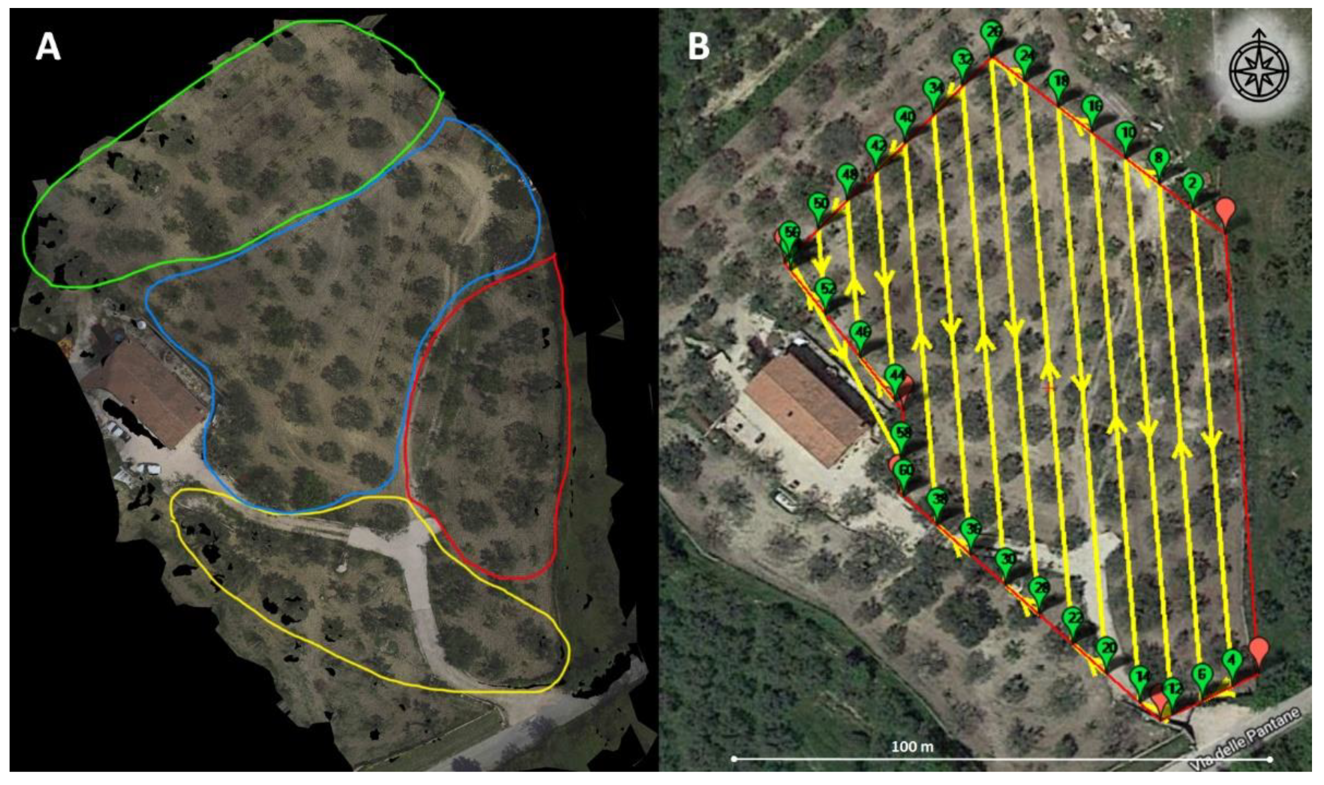
2.2. Experimental Field and Setup

On 22 May 2019 (during flowering) a flight with the UAV DJI Spark (made by DJI SZ DJI Technology Co., Ltd., Shenzhen, China) was performed in a farm (Ponzani Antonio farm), located in Montorio Romano (Central Italy; N 42.1395917; E 12.77265), to make a rough estimation of EVOO production from UAV RGB ortho-photos, using a leaf-area estimation (Datum WGS84). The number of pixels relative to the aerial part per plant has been related to the verified production plant by plant. Three main cultivars were considered: Carboncella (57 olive trees), Frantoio (2 olive trees) and Leccino (15 olive trees). The olive grove is located in the hills. The trees are separated by average distances of 10.2 × 8.9 m, or 110 plants per hectare. The mean height of the plants is 3.27 ± 1.18 m. The surface is composed of an irregular planting layout and is characterized by a slope of 35%. The experimental design and the basic theory on the estimation of biophysical and geometrical parameters of olive trees followed the approach proposed by Caruso et al. [16]. The olive orchard was divided into four plots (Figure 1A) using spatial proximity criterion, where two plots included 18 trees and the remaining two 19 plants each. Three plots were used as a training set for the regression model and one plot was used as a test (Figure 1A). For each region of the training set a regression model was built using only four samples (two small plants with low productivity and two highly productive large plants) and the regression models obtained were finally tested on the test region. The dimension of the plants considered was fixed based on the canopy radius extracted from UAV orthophoto.

2.3. UAV Images Acquisition and Orthoimage Reconstruction

UAV orchard reconstruction was performed starting from an overfly done at a height of 12 m above the ground. The UAV characteristics are visible in Table 1.
The flight of the UAV drone was planned with the open-source Mission Planner software [26]. This software allows for flight design obeying several prescriptions related to the surface to be acquired, such as: e.g., overlap and sidelap, ground sampling distance (GSD), total flight time and image acquisition synchronization. The mission, once appropriately designed, was exported to the application used to flight-control and pilot the UAV (Litchi for Android), (Figure 1B). The application can load waypoints through csv files for a predefined mission flight allowing for photogrammetric applications using a commercial limited budget drone (under 400 €).
The UAV digital camera collected still images every 2.13 s using a shutter speed of 1/5000 s and a sensitivity of 100 ISO. The camera specifications are described in Table 1. Images were collected using the UAV with the digital camera flying with a velocity of 2 ms−1 at 12 m above ground level (AGL) obtaining a GSD (Ground Sample Distance) equal to 0.415 cm/pixel. The experimental flight was conducted on 22 May 2019. The 340 images were acquired with natural light illumination, with a time-lapse with the RGB camera. The total flight time including take-off and landing was about 14 min.
Before flying, an image color checker GretagMacbeth (24 patches) (X-Rite, Grand Rapids, MI, USA) was acquired for later color calibration. The a priori knowledge of the color checker patches values allowed the calibration of all the images following the thin-plate spline interpolation function [27] in the RGB space values following a defined procedure developed in MATLAB [27] (MathWorks Inc., Natick, MA, USA). This method helps to minimize the effects of the illuminants, camera characteristics and settings measuring the ColorChecker‘s RGB coordinates within the acquired images and warping them (transformed) into the known reference coordinates of the ColorChecker.
After image acquisition, the orthophotos were reconstructed using the software “3DF Zephyr” (Zephir 3DFLow 2018, Verona, Italy) [28] according to the following steps: project creation; camera orientation and sparse point cloud generation at high accuracy (100% resolution with no resize); dense point cloud generation; mesh extraction; textured mesh generation; export outcome files (Digital Surface Model—DSM and Digital Terrain Model—DTM) and the orthophoto.

2.4. Leaf Area Estimation

On the original orthorectified UAV image of the whole orchard, a 650 × 650 px bounding box was manually centred on each olive tree of the region considered and the corresponding image extracted. As a result, 74 images (650 × 650 px each) were obtained corresponding to the 74 olive trees considered. For each olive tree, the leaf area was estimated by classifying the pixels of the corresponding 650 × 650 px image and counting the ones belonging to the class ‘’leaves’’. This was done using a kNN supervised learning algorithm adopted to classify the pixels in five classes (“Trunk”, “Leaves”, “Ground”, “Other trees”, “Else”). The kNN algorithm was trained on a dataset built by manually extracting 500 patches (10 × 10 px)—100 for each class—from the original orthorectified UAV image of the whole orchard. The Java tool used for the kNN training was k-PE—kNN Patches Extraction software [29] with k = 7. The normalized leaf area was obtained by counting pixels belonging to the “Leaves” class and dividing by the total area of the 650 × 650 bounding box (4225 px2). The output of the kNN classification filter is a black and white image in which the white pixels are those belonging to the “Leaves” class.

2.5. Canopy Radius Estimation

An original method for the automated canopy radius estimation from the segmented 650 × 650 px kNN image has been implemented. First, the image is read as a matrix M650 × 650 whose elements are 1 for white pixels (leaves), 0 for black pixels (trunk), and 0.5 for gray pixels (rest). At the beginning the center of the canopy’s approximate circumference is C = (325;325) (placed at the centre of the image), and the provisional canopy radius is r = 0. Afterwards, at each step of the algorithm, the provisional radius r is incremented by 1 (up to 325 which corresponds to Rmax) and the matrix elements in the neighbourhood of C are analysed. If matrix elements equal to 1 are found, the coordinates of C are updated as follows:
C x = ( p x m a x p x m i n ) 2
C y = ( p y m a x p y m i n ) 2
where pxmax(min) represents the largest (smallest) column index of the matrix element whose value is 1 and pymax(min) the largest (smallest) row index of the matrix element whose value is 1. As a result, at each step, the centre C moves all around the picture and r increases. The algorithm converges when no new 1 matrix elements are found, and the canopy radius R is obtained as:
R = c x L + c y L 2 .
In Equation (3) c x L and c y L the coordinate of C in the last iteration. The Matlab code is reported in Appendix A.

2.6. Olive and EVOO Production Estimation

For each olive tree in the four regions the total olives produced were weighed. These regions were chosen following a proximity criterion (Section 2.2). At harvest (carried out from 7 to 27 November), the olives were weighed inside the mill. The total weight per cultivar and the corresponding average yields are reported in Table 2.
The total weight was recorded for the three cultivars harvested equalled 3167.5 kg for Carboncella, 74 kg for Frantoio and 704.5 kg for Leccino, for a total weight of 3946 kg. The productivity of each region was analysed using a two-classes k-means unsupervised classification algorithm, which outputs two subsets characterized by high and low productivity. Thus, the productivity values were plotted against the predicted canopy radius R of Formula (3). For each region only four samples were used: two samples belonging to the low-productivity subset and having smallest values of R/Rmax and two samples belonging to the high-productivity subset and having largest values of R/Rmax. On these four samples a linear regression model was applied considering as independent variable x = R/Rmax and y = log10(p/P0 + 1) as dependent one.
l o g 10 ( p / P 0 + 1 ) = a ( R R m a x ) + b
In Equation (4) p is the estimated production in kg, R/Rmax is the canopy radius normalized to half of the image size, a and b are fitting parameters and P0 = 1 kg is a dimensional constant. The factor 1 is necessary for the argument of the logarithm being zero when p = 0. The total production estimates for every single region were obtained by summing up the predicted values of p.
The EVOO production estimate was obtained by multiplying the predicted production in Kg of the single plant by the relative average yield.

3. Results

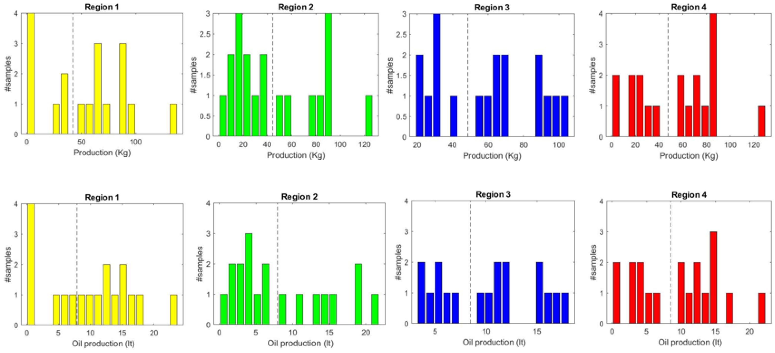
3.1. Loading and Unloading Subsets

The four regions showed a clear distinction between highly productive and low productive plants, demonstrating the tendency of olive trees to have loading and unloading years of production [26].
Figure 2 shows the plant production (Figure 2 top) and the EVOO production (Figure 2 down) of the four regions of the orchard (Yellow, Green, Blue and Red) considered. It is possible to observe that in all productivity histograms (Figure 2 top) there is a clear gap between the high productivity region and low productivity region of the plot. As a result, for every single region considered, the data can be grouped into two distinct subsets separated by a boundary. The precise location of this boundary was calculated with the K-means clustering algorithm (see below) and is located at about 45 kg in the olive production histogram. The corresponding boundary for the oil production histogram was obtained considering the average yield reported in Table 3 and has a value of approximately eight litres.

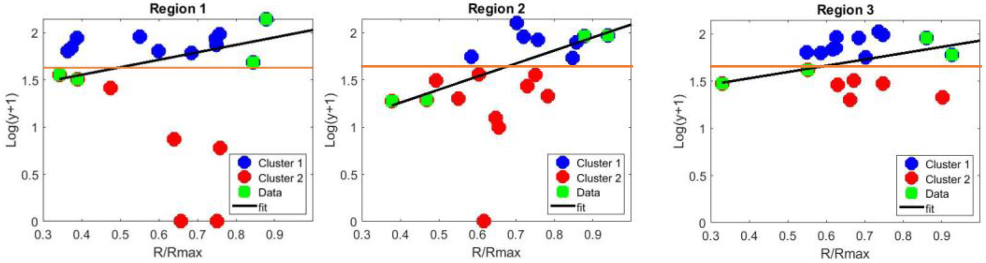
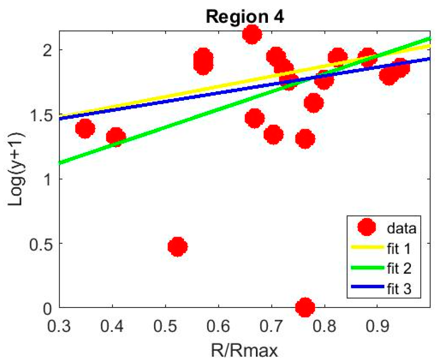
3.2. Leaf Area and Canopy Radius Estimate from kNN Image Segmentation

In order to predict the total production of a region of the orchard, it is necessary to correlate it with a measurable quantity. The reasonable measurable parameters considered are the leaf area and the canopy radius. Indeed, one expects “on average” larger plants to produce more olives. The basis of this assumption is that the density of olives (olive weight divided by the canopy volume) is spherically symmetric and it does not decrease faster than (R/Rmax)−3. Given the age of the orchard and its agronomic conditions, the above assumption seems to be reasonable and was verified a posteriori (see Figures 4 and 5). The use of modern technology, particularly UAV orthophotos, allows good estimation of plant characteristics such as the normalized difference vegetation index (NDVI), leaf area, and canopy volume [14]. In particular, the canopy radius could be even manually identified on the orthophoto and measured compared to the picture size. The canopy radius and the leaf area estimates were simultaneously obtained adopting the automated method described in Section 2 (see also Appendix A).
Figure 3 shows the picture of an olive tree extracted from the UAV orthophoto (Figure 3a), segmented with the kNN algorithm (Figure 3b) and its canopy circumference (Figure 3c) given the canopy radius extracted with the algorithm described in Section 2.
To give an estimate of the olive regional productivity both the leaf area and the canopy radius assessed from the UAV orthophoto reconstruction can be used. However, for all the four regions considered it was found that the normalized leaf area is quadratically correlated with the canopy radius. In particular, the regression equation holds, where NLA stands for normalized leaf area and x = R/Rmax was already defined above. The regression coefficients m and q are reported in Table 3 for the four regions analysed.
N L A = m x 2 + q
Given these results, in principle it is irrelevant which variable is chosen for describing the system (leaf area or x = R/Rmax). However, the overall kNN pixel classifier accuracy is 71.3% and pixel misclassification can occur. Conversely, very few pixels are needed to draw the canopy circumference. As a result, although leaf area estimation for the individual tree may be inaccurate, the canopy boundary is detected very well and consequently the normalized canopy radius was considered an independent variable. Moreover, the canopy radius can be directly measured in-field and can be used both as an external test for the model and as an input for the production estimate protocol.
Note that the estimated leaf area was not reported since it was not used for estimating the olive production. The main result of Equation (5) is indeed that the leaf area is proportional to the square of the canopy radius. This justifies the use of the canopy radius (which is easier to measure with respect to the leaf area) for estimating the olive production.
First of all, for each region among the three chosen as training for the model, the productivity as a function of the normalized canopy radius was plotted in a logarithmic scale (Figure 4) and the data were analysed by means of a k-means clustering algorithm. In this way, it is possible to separate the highly productive plants (loading) from the unloading one (see Section 3.1). When plotted in logarithmic scale, all the three regions show a gap between the two subsets located at around log10(p/P0 + 1) = 1.65 which corresponds to p = 45 kg in agreement with the results of Section 3.1. The following procedure was then applied to the three regions of the training set. Among the low productive plants two plants with the smallest R/Rmax were considered, and among the highly productive plants two plants with the largest canopy radius were considered. These four samples are marked as green squares in Figure 4 and were used to build the regression model defined by Equation (4). In Table 4 the fitting parameters, the determination coefficients and the production estimates are reported for the three regions considered as training.
For the three regions considered as training, the estimated productivity for the olive weight resides in an interval (−11.5%, +2.8%) and that for the EVOO resides in an interval (−11.5%, +2.3%). At this point the fourth region was used as a validation test for the regression (Figure 5). In this way it is possible to give a sort of confidence interval of the estimates obtained.
The productivity and EVOO estimates for Region 4 obtained using the regression coefficients of the other three regions are reported in Table 5.
The estimated productivity for both the olive weight resides in an interval (−3.8%, 16.7%), slightly smaller than that for the EVOO which resides in an interval (−3%, 17.6%).

4. Discussion and Conclusions

The purpose of the article is the evaluation of the olives and EVOO production through the canopy radius extracted from orthophoto acquired by a UAV. The flight was performed in May since in the period between May and June there is the maximum flowering of olive trees and the beginning of the growth of the fruits. Therefore, it has been demonstrated that flowering is a good period for making an accurate early estimate of the production [25,26]. Indeed, the chosen period coincides with the flowering phase and is the earliest period to be able to estimate crop productivity. In future research we would like to replicate the same approach by considering different periods, from flowering onwards, to see which period can best approximate the production estimate.
Light drone applications [15,30] are increasing their importance due to reduced budgets and the possibility of flying with a reduced need for bureaucratic permissions. The use of UAVs for crop phenotyping of plants is rapidly growing [31] because of the difficulty involved and the precision limit of manual crop analysis [20,32,33].
Yield production in olive trees was studied as a function of row spacing [e] and canopy volume [d]. However, ref. [32] is a preliminary study and only 16 samples were considered. Yield production estimates seem to be more efficient in herbaceous crops.
Nevavouri et al. [31], used a convolutional neural network (CNN) based on NDV and RGB data acquired from UAVs to predict wheat and barley yield. Results indicate that the best performing model can predict within-field yield with an average absolute error of 484 kg/ha (MAPE: 8.8%) based only on RGB images in the early stages of growth (<25% of total thermal time). The model for RGB images in later growth stages returned higher error values (MAE: 680 kg/ha; MAPE: 12.6%). Another study involving the estimation and analysis of above-ground biomass (AGB) of the wheat crop using a consumer-grade red-green-blue (RGB) camera mounted on a drone is that of Panday et al. [34]. AGB and wheat yield were estimated by linear regression models through plant height obtained from crop area models from images captured by the drone-mounted camera. The plant height estimated from the drone images had an error between 5% and 11.9% compared to the direct field measurement.
Future work could lead to the streamlining of the processing operation in order to produce a practical application ready to use. Nevertheless, the process can be streamlined and automated for easy operation and data analysis. This work represents one step among several currently being used that are shifting agricultural management from precision farming towards digital farming [30,31,32,33].
Figure 2 shows a histogram of the plant production. It is possible to observe a clear gap between the high productivity (loading year) region and low productivity (unloading year) for each region of the plot. As reported by Ramos-Román [25], the olive tree is a climatic-sensitive tree taxon conditioned by the present aridification tendency in the Mediterranean climate areas. Indeed, it is a common experience that olive tree production tends to oscillate from year to year, leaving the overall productivity of the orchard almost constant in time [26]. Generally, some varieties of olive trees provide alternation of a productive year (loading) followed by a year of discharge (unloading). This could be caused by certain climatic conditions and agronomic techniques, such as pruning, fertilization and irrigation [34]. This feature also is also reflected in olive oil production. Figure 2 shows that the population of the two subsets varies among the four regions. In particular, the unbalanced ratio between loading and unloading years among the three regions considered as training does not affect the overall performance. This demonstrated the validity of the proposed model. Frauds regarding food distribution is a great problem in modern society. Extra virgin olive oil is one of the products with a higher percentage of sophisticated imitations. One way to fight against EVOO sophistications is to guarantee the continuity from producer to consumer. A correct production estimate, also for table olives, could be useful for the planning of industrial processes which the drupes undergo after harvesting (e.g., debittering). In this respect it is important that the declared production reasonably corresponds to the real one.
In this paper an effective and scalable method for giving an accurate estimate of the production of olive orchards has been proposed. The method shown here takes as input UAV pictures of the orchard and the real production of a few plants of the orchard. The UAV orthophoto is then cropped around the olive trees and segmented with a kNN algorithm. At this point, a counting algorithm automatically extracts the normalized leaf area, the canopy radius and the canopy center. Applying a k-means classification to the graph of the production measured in kilograms as a function of R, two distinct zones emerged, associated with the year of loading (high production) and the year of unloading (low production), respectively. The total production estimated by the aforementioned regression model deviates from the real one by less than 12% in training and less than 18% in test. This makes the estimation of total production according to the canopy radius assessed by orthophotos robust and reliable, and makes it possible to draw up an anti-fraud protocol about the declared production, knowing the number of plants and their extension. The proposed methodology could help farmers in tracking the production amount per field zone, identifying eventual problems or aiding in defining a production and marketing strategy in advance. Future works, also thanks to the unsupervised nature of the K-means clustering machine learning algorithm, could interestingly point to a streamlining of the acquisition and analysis protocols on one side and the testing of a drone equipped with a higher resolution sensor to increase the performances on the other. Once the acquisition and analysis flow has been strengthened, the whole system could be applied as a practical anti-fraud protocol on the basis of the declared production towards sample farms.

Author Contributions

Conceptualization, L.O. and C.C.; methodology, L.O., S.V. (Simona Violino); software, S.F., S.V. (Simone Vasta), F.T., L.O.; validation, L.O., S.V. (Simona Violino) and C.C.; formal analysis, L.O., S.V. (Simona Violino), G.I. and C.C.; investigation, L.O., S.V. (Simona Violino), G.I.; resources, L.O. and S.V. (Simona Violino); data curation, L.O., S.V. (Simona Violino) and G.I.; writing—original draft preparation, L.O. and S.V. (Simona Violino); writing—review and editing, L.O., S.V. (Simona Violino), F.A., F.P. and C.C.; visualization, L.O., S.V. (Simona Violino), F.A., F.P. and C.C.; supervision, C.C. and F.P.; project administration, C.C. and F.P.; funding acquisition, C.C. and F.P. All authors have read and agreed to the published version of the manuscript.

Funding

This paper was funded with the contribution of the Italian Ministry of Agricultural, Food, Forestry and Tourism Policies (MiPAAFT) sub-project “Tecnologie digitali integrate per il rafforzamento sostenibile di produzioni e trasformazioni agroalimentari (AgroFiliere)” (AgriDigit program) (DM 36503.7305.2018 of 20/12/2018), developed also within the project INFOLIVA (D.M. n.12479), the project INNOLITEC (D.M. 37067/2018) and the project DEAOLIVA (D.M. n. 93882/2017).

Institutional Review Board Statement

Not available.

Informed Consent Statement

Not available.

Data Availability Statement

Not available.

Acknowledgments

The authors wish to thank the Azienda Agricola di Ponzani Antonio—Montorio Romano (RM) for the valuable support shown in the acquisition of data in the field and for the availability. L.O. acknowledges Giulio Cimini for illuminating discussions on allometric scaling equations and Giuseppe Ortenzi for the practical teaching of pruning technique of olive trees.

Conflicts of Interest

The authors declare no conflict of interest.

Appendix A

Matlab code for obtaining the canopy radius, canopy center and leaf area from images segmented with an image segmentation algorithm (in this case kNN).
clear all;
close all;
clc
DINPUT = ‘Directory\where\the\segmented\pictures\are\’; %DIR di input
files = dir([DINPUT ‘*.png’]);
L = length(files);
Rmax = zeros(L,1);
for k = 1:L, % cicle over the files
fname = files(k).name;
B = im2double(imread([DINPUT fname])); % input segmented image size(B) = [650,650];
IMGR = repmat(B,[1,1,3]); % make an RGB from segmented image
ny = size(B,1); % n rows
nx = size(B,2); % n columns
C1 = round(nx/2); % initial coordinates
C2 = round(ny/2); % of the Center.
R = min(C1,C2); % Radius
%%% making B binary %%%
reshape(B,size(B,1)*size(B,2),1);
for i = 1:size(B,1)*size(B,2)
if (B(i) < 1)
B(i) = 0;
else
B(i) = 1;
end
end
%%% initialize variables %%%
nump = zeros(1,round(R));
JMAX = C2;
IMAX = C1;
Imin = IMAX;
Jmin = JMAX;
%%%
for r = 1:1:R
kk = 0;
reshape(B,size(B,1),size(B,2));
for i = 1:1:nx %column index
for j = 1:1:ny %row index
if(((j-C2)^2 + (i-C1)^2) < r^2 && B(j,i) > 0.5)
kk = kk + 1; %counts how many leaves
%%% AVOIDS DOUBLE COUNTING!!! %%%
B(j,i) = 0.3; %%%MARK THIS POINT%%%
%%% !!!!!IMPORTANT!!!! %%%
if (i > IMAX)
IMAX = i;
end
if (j > JMAX)
JMAX = j;
end
if (i < Imin)
Imin = i;
end
if (j < Jmin)
Jmin = j;
end
end
end %i
end %j
nump(r) = kk;% between r−1 and r there are kk leaves!!!
end% r
data(k,1) = sum(nump)/nx/ny; % leaf area automatically comes out!
C1 = ((IMAX-Imin)/2);
C2 = ((JMAX-Jmin)/2);
R = (C1 + C2)/2;
C1 = floor(C1 + Imin);
C2 = floor(C2 + Jmin);
Rmax(k) = R;
fprintf(‘Leaf area =%d Canopy radius =%d ‘, data(k,1),2*Rmax(k)/nx);
fprintf(‘Canopy center = [%d %d]\n’,C2,C1);
%%% Just for plot %%%
for i = 1:1:nx
for j = 1:1:ny
if (((j-C2)^2 + (i-C1)^2) < (R + 2)^2 && ((j-C2)^2 + (i-C1)^2) > (R−2)^2 )
IMGR(j,i,:) = [0,255,0];
end
end
end
IMGR(C2-2:C2 + 2,C1-2:C1 + 2,1) = ones(5,5);
IMGR(C2-2:C2 + 2,C1-2:C1 + 2,2) = zeros(5,5);
IMGR(C2-2:C2 + 2,C1-2:C1 + 2,3) = zeros(5,5);
imshow(imresize(IMGR,[300,300]));
pause;
%%%
end

References

  1. Violino, S.; Pallottino, F.; Sperandio, G.; Figorilli, S.; Ortenzi, L.; Tocci, F.; Vasta, S.; Imperi, G.; Costa, C. A Full Technological Traceability System for Extra Virgin Olive Oil. Foods 2020, 9, 624. [Google Scholar] [CrossRef]
  2. Cajka, T.; Riddellova, K.; Klimankova, E.; Cerna, M.; Pudil, F.; Hajslova, J. Traceability of olive oil based on volatiles pattern and multivariate analysis. Food Chem. 2010, 121, 282–289. [Google Scholar] [CrossRef]
  3. Violino, S.; Pallottino, F.; Sperandio, G.; Figorilli, S.; Antonucci, F.; Ioannoni, V.; Fappiano, D.; Costa, C. Are the Innovative Electronic Labels for Extra Virgin Olive Oil Sustainable, Traceable, and Accepted by Consumers? Foods 2019, 8, 529. [Google Scholar] [CrossRef] [Green Version]
  4. Vecchio, R.; Annunziata, A. The role of PDO/PGI labelling in Italian consumers’ food choices. Agric. Econ. Rev. 2011, 12, 80–89. [Google Scholar]
  5. Cicia, G.; Cembalo, L.; Del Giudice, T. Country-of-origin effects on German peaches consumers. New Medit. 2012, 11, 75–79. [Google Scholar]
  6. Lanza, B.; Di Serio, M.G.; Iannucci, E.; Russi, F.; Marfisi, P. Nutritional, textural and sensorial characterisation of Italian table olives (Olea europaea L. cv.‘Intosso d’Abruzzo’). Int. J. Food SCi. Technol. 2010, 45, 67–74. [Google Scholar] [CrossRef]
  7. Di Vita, G.; D’Amico, M.; La Via, G.; Caniglia, E. Quality Perception of PDO extra-virgin Olive Oil: Which attributes most influence Italian consumers? Agric. Econ. Rev. 2013, 14, 46–58. [Google Scholar]
  8. Tseng, T.H.; Balabanis, G. Explaining the product-specificity of country-of-origin effects. Int. Mark. Rev. 2011, 28, 581–600. [Google Scholar] [CrossRef]
  9. Poiana, M.A.; Alexa, E.; Munteanu, M.F.; Gligor, R.; Moigradean, D.; Mateescu, C. Use of ATR-FTIR spectroscopy to detect the changes in extra virgin olive oil by adulteration with soybean oil and high temperature heat treatment. Open Chem. 2015, 13, 1. [Google Scholar] [CrossRef]
  10. Agrimonti, C.; Vietina, M.; Pafundo, S.; Marmiroli, N. The use of food genomics to ensure the traceability of olive oil. Trends Food Sci. Technol. 2011, 22, 237–244. [Google Scholar] [CrossRef]
  11. Bontempo, L.; Paolini, M.; Franceschi, P.; Ziller, L.; García-González, D.L.; Camin, F. Characterisation and attempted differentiation of European and extra-European olive oils using stable isotope ratio analysis. Food Chem. 2019, 276, 782–789. [Google Scholar] [CrossRef]
  12. Guido, R.; Mirabelli, G.; Palermo, E.; Solina, V. A framework for food traceability: Case study–Italian extra-virgin olive oil supply chain. Int. J. Ind. Eng. Manag. 2020, 11, 50–60. [Google Scholar] [CrossRef]
  13. Bianchini, A. A Blockchain-Based System for LoT-Aided Certification and Traceability of EVOO. 2018. Available online: https://etd.adm.unipi.it/theses/available/etd-08312018-174046/unrestricted/tesi.pdf (accessed on 6 September 2021).
  14. Miranda-Fuentes, A.; Llorens, J.; Gamarra-Diezma, J.L.; Gil-Ribes, J.A.; Gil, E. Towards an optimized method of olive tree crown volume measurement. Sensors 2015, 15, 3671–3687. [Google Scholar] [CrossRef] [Green Version]
  15. Fanigliulo, R.; Antonucci, F.; Figorilli, S.; Pochi, D.; Pallottino, F.; Fornaciari, L.; Grilli, R.; Costa, C. Light Drone-Based Application to Assess Soil Tillage Quality Parameters. Sensors 2020, 20, 728. [Google Scholar] [CrossRef] [Green Version]
  16. Caruso, G.; Zarco-Tejada, P.J.; Gonzalez-Dugo, V.; Moriondo, M.; Tozzini, L.; Palai, G.; Rallo, G.; Hornero, A.; Primicerio, J.; Gucci, R. High-resolution imagery acquired from an unmanned platform to estimate biophysical and geometrical parameters of olive trees under different irrigation regimes. PLoS ONE 2019, 14, e0210804. [Google Scholar] [CrossRef] [Green Version]
  17. Díaz-Varela, R.A.; De la Rosa, R.; León, L.; Zarco-Tejada, P.J. High-resolution airborne UAV imagery to assess olive tree crown parameters using 3D photo reconstruction: Application in breeding trials. Remote Sens. 2015, 7, 4213–4232. [Google Scholar] [CrossRef] [Green Version]
  18. Torres-Sánchez, J.; López-Granados, F.; Serrano, N.; Arquero, O.; Peña, J.M. High-throughput 3-D monitoring of agricultural-tree plantations with unmanned aerial vehicle (UAV) technology. PLoS ONE 2015, 10, e0130479. [Google Scholar] [CrossRef] [Green Version]
  19. Zarco-Tejada, P.J.; Diaz-Varela, R.; Angileri, V.; Loudjani, P. Tree height quantification using very high resolution imagery acquired from an unmanned aerial vehicle (UAV) and automatic 3D photo-reconstruction methods. Eur. J. Agron. 2014, 55, 89–99. [Google Scholar] [CrossRef]
  20. Rallo, P.; de Castro, A.I.; López-Granados, F.; Morales-Sillero, A.; Torres-Sánchez, J.; Jiménez, M.R.; Casanova, L.; Suárez, M.P. Exploring UAV-imagery to support genotype selection in olive breeding programs. Sci. Hortic. 2020, 273, 109615. [Google Scholar] [CrossRef]
  21. Cheng, Z.; Qi, L.; Cheng, Y.; Wu, Y.; Zhang, H. Interlacing orchard canopy separation and assessment using UAV images. Remote Sens. 2020, 12, 767. [Google Scholar] [CrossRef] [Green Version]
  22. Park, S.; Ryu, D.; Fuentes, S.; Chung, H.; Hernández-Montes, E.; O’Connell, M. Adaptive estimation of crop water stress in nectarine and peach orchards using high-resolution imagery from an unmanned aerial vehicle (UAV). Remote Sens. 2017, 9, 828. [Google Scholar] [CrossRef] [Green Version]
  23. Bertrad, E. The beneficial cardiovascular effects of the Mediterranean diet. Olivae 2002, 90, 29–31. [Google Scholar]
  24. Deidda, P.; Nieddu, G.; Chessa, I. La Fenologia. In Olea Trattato di Olivicoltura; Fiorino, P., Ed.; Edagricole: Bologna, Italy, 2003; pp. 57–73,461. [Google Scholar]
  25. Ramos-Román, M.J.; Jiménez-Moreno, G.; Anderson, R.S.; García-Alix, A.; Camuera, J.; Mesa-Fernández, J.M.; Manzano, S. Climate controlled historic olive tree occurrences and olive oil production in southern Spain. Glob. Planet. Chang. 2019, 182, 102996. [Google Scholar] [CrossRef]
  26. Oborne, M. Mission Planner. 2015. Available online: http://planner.ardupilot.com (accessed on 6 September 2021).
  27. Menesatti, P.; Angelini, C.; Pallottino, F.; Antonucci, F.; Aguzzi, J.; Costa, C. RGB color calibration for quantitative image analysis: The “3D Thin-Plate Spline” warping approach. Sensors 2012, 12, 7063–7079. [Google Scholar] [CrossRef] [Green Version]
  28. Anwar, N.; Izhar, M.A.; Najam, F.A. Construction monitoring and reporting using drones and unmanned aerial vehicles (UAVs). In Proceedings of the Tenth International Conference on Construction in the 21st Century (CITC-10), Colombo, Sri Lanka, 2–4 July 2018; pp. 2–4. [Google Scholar]
  29. Pallottino, F.; Menesatti, P.; Figorilli, S.; Antonucci, F.; Tomasone, R.; Colantoni, A.; Costa, C. Machine vision retrofit system for mechanical weed control in precision agriculture applications. Sustainability 2018, 10, 2209. [Google Scholar] [CrossRef] [Green Version]
  30. Guijun, Y.; Liu, J.; Zhao, C.; Li, Z.; Huang, Y.; Yu, H.; Xu, B.; Yang, X.; Zhu, D.; Zhang, X.; et al. Unmanned aerial vehicle remote sensing for feld-based crop phenotyping: Current status and perspectives. Front. Plant Sci. 2017, 8, 1111. [Google Scholar] [CrossRef]
  31. Paulus, S. Measuring crops in 3D: Using geometry for plant phenotyping. Plant Methods 2019, 15, 103. [Google Scholar] [CrossRef] [PubMed]
  32. Torres-Sánchez, J.; de la Rosa, R.; León, L.; Jiménez-Brenes, F.M.; Kharrat, A.; López-Granados, F. Quantification of dwarfing effect of different rootstocks in ‘Picual’ olive cultivar using UAV-photogrammetry. Precis. Agric. 2021. [Google Scholar] [CrossRef]
  33. Nevavuori, P.; Narra, N.; Lipping, T. Crop yield prediction with deep convolutional neural networks. Comput. Electron. Agric. 2019, 163, 104859. [Google Scholar] [CrossRef]
  34. Panday, U.S.; Shrestha, N.; Maharjan, S.; Pratihast, A.K.; Shrestha, K.L.; Aryal, J. Correlating the plant height of wheat with above-ground biomass and crop yield using drone imagery and crop surface model, a case study from Nepal. Drones 2020, 4, 28. [Google Scholar] [CrossRef]
Figure 1. (A) Location map with the four plots. The red plot has been used as test; (B) Mission planned with the open source “Mission Planner”.
Drones 05 00118 g001
Figure 2. Top -from left to right- olive productivity histogram for the four regions of the orchard (yellow, green, blue and red). Bottom, from left to right, oil productivity histogram for the four regions of the orchard (yellow, green, blue and red). The dashed lines represent the boundaries between the loading year and unloading year region of the plot, calculated with the k-means algorithm.
Drones 05 00118 g002
Figure 3. (a) Image of the olive tree before image segmentation; (b) Image segmented with kNN supervised learning algorithm; (c) Calculated canopy circumference having radius R. The patches assigned to the class “leaves” by the kNN algorithm are marked in red.
Drones 05 00118 g003
Figure 4. Regional productivity in logarithmic scale as a function of the normalized canopy radius for the three regions considered as training for the model. The data were divided into two subsets by a k-means clustering algorithm (blue and red circles). Four points (green squares) were chosen to perform a linear regression—see Equation (4)—(black line).
Drones 05 00118 g004
Figure 5. Productivity in logarithmic scale as a function of the normalized canopy radius of Region 4 (red circles). The productivity estimates (both for the olive weight and for the EVOO) were obtained using the regression models of training Region 1 (yellow line), Region 2 (green line) and Region 3 (blue line). The parameters of the fitting lines are reported in Table 4.
Drones 05 00118 g005
Table 1. Specifications of the unmanned aerial vehicle (UAV) DJI™ SPARK™.
DetailsItemsSpecifications
UAVWeight297 g
Dimensions143 mm × 143 mm × 55 mm
Max speed50 km/h
Satellite positioning systemsGPS/GLONASS
Digital cameraCamera Focal length4.5 mm
Sensor dimensions (W × H)6.17 mm × 4.56 mm
Sensor Resolution12 megapixels
Image Sensor TypeCMOS
Capture FormatsMP4 (MPEG-4 AVC/H.264)
Still Image FormatsJPEG
Video Recorder Resolutions1920 × 1080 (1080 p)
Frame Rate30 frames per second
Still Image Resolutions3968 × 2976
GIMBALControl range Inclinationfrom −85° to 0°
StabilizationMechanical 2 axes (inclination, roll)
Obstacle detection distance0.2–5 m
Operating environmentSurfaces with diffuse reflectivity (>20%) and dimensions greater than 20 × 20 cm (walls, trees, people, etc.)
Remote ControlOperating Frequency5.8 GHz
Max Operating Distance1.6 km
BatterySupported Battery
Configurations
3S
Rechargeable BatteryRechargeable
Technologylithium polymer
Voltage Provided11.4 V
Capacity1480 mAh
Run Time (Up to)16 min
Recharge Time52 min
Table 2. Total regional weight (Kg) and average yield per cultivar.
Region 1 (kg)Region 2 (kg)Region 3 (kg)Region 4 (kg)Average Yield (lt/hw)
Carboncella691.5627.01021.5827.517.2
Leccino284.5258.529.0132.520
Frantoio0.011.50.062.517.8
Total976.0897.01050.51022.5
Table 3. Regression coefficients of Equation (5).
Region 1Region 2Region 3Region 4
m0.420.450.360.45
q0.01−0.04−0.01−0.03
Coefficient of determination R20.870.800.930.78
Table 4. Results of the production estimate procedure for the three regions of the training set obtained through the regression Equation (4).
Region 1Region 2Region 3
a (see Equation (4))0.79311.38360.6662
b (see Equation (4))1.23880.70651.2651
Coefficient of determination R20.62200.97870.8007
Predicted weight (kg)976.7922.4936.1
Measured weight (kg)976.0897.01050.5
% error on the weight1.02.8−11.5
Predicted EVOO (lt)174.2165.4161.8
Meaure EVOO175.8161.6181.5
Table 5. Production and EVOO estimates obtained using the regression coefficients of the three regions considered as training.
Predicted Weight (kg)% Error on the WeightPredicted EVOO (IT)EVOO
Error%
Region 11208.916.7214.717.6
Region 2984.7−3.8174.7−3.0
Region 31032.70.99180.01.9
Publisher’s Note: MDPI stays neutral with regard to jurisdictional claims in published maps and institutional affiliations.

