Data for Heuristic Optimization of Electric Vehicles’ Charging Configuration Based on Loading Parameters


1
Boysen-TU Dresden-Research Training Group, Electrical Power Supply, Technical University of Dresden, 01069 Dresden, Germany
2
Electrical Power Supply, Technical University of Dresden, 01069 Dresden, Germany
*
Author to whom correspondence should be addressed.
Data 2020, 5(4), 102; https://doi.org/10.3390/data5040102
Submission received: 13 October 2020
/
Revised: 23 October 2020
/
Accepted: 26 October 2020
/
Published: 29 October 2020
Abstract
:This dataset includes multiple files related to optimization of electric vehicles to minimize overloading in low voltage grids by varying the locations available to charge the EVs. The data include lognormally sampled hourly sorted scenarios across 11 charging locations for a stochastics-based Monte Carlo simulation. This simulation runs through 2 million scenarios based on actual probabilities to incorporate most possible situations. It also includes samples from normally distributed household electricity use scenarios based on agent-based modeling. The article includes the test grid parameters for simulation, which were used to create a benchmark grid in DigSilent Powerfactory software, as well as intermediate outputs defining worst case scenarios when electric vehicles were charged and results from three different optimization approaches involving a reduction in voltage drops, cable overloading and total line losses. The outputs from the benchmark grid were used to train a machine learning algorithm, the weights and codes for which are also attached. This trained network acted as the grid for subsequent iterative optimization procedures. Outputs are presented as a comparison between pre-optimization and post-optimization scenarios. The above dataset and procedure were repeated while varying the number of EVs between 0 and 100 in increments of 20, data for which are also attached. The data article supports a related submission titled “Minimization of Overloading Caused by Electric Vehicle (EV) Charging in Low Voltage Networks”.
Dataset: Haider, Sajjad (2020), “Data for Optimization of Electric Vehicle Charging Configuration to Reduce Overloading in Low Voltage Networks”, Mendeley Data, V3, doi:10.17632/6yvzmnpb9h.3
Dataset License: (CC-BY)
1. Summary
Data are specifically designed to allow Monte Carlo analyses of future electrified transport based on typical European grids and population demographics. Typical Monte Carlo analysis incorporates hundreds of thousands of situations, which are most representative of real world conditions. The authors have run this following model through 0.2 million simulations per hour to ensure the results represent a high confidence interval. This includes probabilities of plugging and unplugging typical household electronics as well as electric vehicles. Researchers looking at better optimization techniques applied to electric vehicle charging configuration can use the consumer usage profiles inbuilt into the data to compare results against existing and proposed approaches. The data can be used to set up a similar network and user profiles to study the impact of allowing household charging v. communal charging. It can also be used to study the implications of allowing unused electric vehicles to sell electricity back to the grid to offset overloading characteristics. The data allow for a probabilistic model of a typical community to be made to study the effects of increasing electric vehicle penetration. Such policies are being propagated as a solution for climate change; however, brute force applications may overburden existing low voltage networks. In cases of higher electric vehicle penetrations, low voltage networks are often overloaded and show significant voltage drops. This might result in the need for significant cable upgrades across the network if optimized charging techniques such as the results compiled in the dataset are not used. By using the approach and data given, models can be built to encourage optimized charging methods, such as by introducing spatial pricing based on the overloading caused by charging electric vehicles at specific locations.
2. Data Description
2.1. Scenarios for Household Electricity Consumption Modelling
- ○
- Singlemanwithwork.xlsx
- ▪
- Sheet 1: Singlemanwithwork provides energy consumption values on an hourly basis for a hypothetical household with a resident couple and one minor:
- Column A is the total minute count in the day.
- Columns B, C and D show the date, hour of the day and minute of the hour of the simulation respectively.
- Column E shows the power reading (in kW) taken at a resolution of 1 min.
- Column F shows the energy consumed in the last one hour. Data are written at the start of every hour corresponding to column C.
- Rows represent individual samples
- ▪
- Sheet 2: Sorted
- Columns A to NB represent individual days of the year while rows 1 to 24 represent the hour of the day for that sample. The values show energy consumption in kWh in that sample.
- ▪
- Sheet 3: Weekends is filtered from the raw data to include only weekends.
- Columns A to DA represent individual weekend days (Saturday and Sunday). while rows 1 to 24 represent hour of the day for that sample. The values show energy consumption in kWh in that sample.
- ▪
- Sheet 4: Weekdays is filtered from the raw data to include only weekdays.
- Columns A to IR represent individual non-weekend days (Monday to Friday) while rows 1 to 24 represent hour of the day for that sample. The values show energy consumption in kWh in that sample.
- ○
- Singlemanwithoutwork.xlsx
- ▪
- Sheet 1: Singlemanwithoutwork provides energy consumption values on an hourly basis for a hypothetical household with a resident single person who is unemployed:
- Column A is the total minute count in the day.
- Columns B, C and D show the date, hour of the day and minute of the hour of the simulation respectively.
- Column E shows the power reading (in kW) taken at a resolution of 1 min
- Column F shows the energy consumed in the last one hour. Data are written at the start of every hour corresponding to column C.
- Rows represent individual samples.
- ▪
- Sheet 2: Sorted
- Columns A to JA represent individual days of the year while rows 1 to 24 represent the hour of the day for that sample. The values show energy consumption in kWh in that sample.
- ▪
- Sheet 3: Weekends is filtered from the raw data to include only weekends.
- Columns A to CZ represent individual weekend days (Saturday and Sunday) while rows 1 to 24 represent hour of the day for that sample. The values show energy consumption in kWh in that sample.
- ▪
- Sheet 4: Weekdays is filtered from the raw data to include only weekdays.
- Columns A to JA represent individual non-weekend days (Monday to Friday) while rows 1 to 24 represent hour of the day for that sample. The values show energy consumption in kWh in that sample.
- ○
- Couplewithwork.xlsx
- ▪
- Sheet 1: Couplewithwork provides energy consumption values on an hourly basis for a hypothetical household with a resident couple and one minor:
- Column A is the total minute count in the day.
- Columns B, C and D show the date, hour of the day and minute of the hour of the simulation respectively.
- Column E shows the power reading (in kW) taken at a resolution of 1 min.
- Column F shows the energy consumed in the last one hour. Data are written at the start of every hour corresponding to column C.
- Rows represent individual samples.
- ▪
- Sheet 2: Sorted
- Columns A to NB represent individual days of the year while rows 1 to 24 represent the hour of the day for that sample. The values show energy consumption in kWh in that sample.
- ▪
- Sheet 3: Weekends is filtered from the raw data to include only weekends.
- Columns A to CZ represent individual weekend days (Saturday and Sunday) while rows 1 to 24 represent hour of the day for that sample. The values show energy consumption in kWh in that sample.
- ▪
- Sheet 4: Weekdays is filtered from the raw data to include only weekdays
- Columns A to JA represent individual non-weekend days (Monday to Friday) while rows 1 to 24 represent hour of the day for that sample. The values show energy consumption in kWh in that sample.
- ○
- Couplewithoutwork.xlsx
- ▪
- Sheet 1: Couplewithoutwork provides energy consumption values on an hourly basis for a hypothetical household with a resident couple and one minor:
- Column A is the total minute count in the day.
- Columns B, C and D show the date, hour of the day and minute of the hour of the simulation respectively.
- Column E shows the power reading (in kW) taken at a resolution of 1 min.
- Column F shows the energy consumed in the last one hour. Data are written at the start of every hour corresponding to column C.
- Rows represent individual samples.
- ▪
- Sheet 2: Sorted
- Columns A to NB represent individual days of the year while rows 1 to 24 represent the hour of the day for that sample. The values show energy consumption in kWh in that sample.
- ▪
- Sheet 3: Weekend is filtered from the raw data to include only weekends.
- Columns A to DJ represent individual weekend days (Saturday and Sunday) while rows 1 to 24 represent hour of the day for that sample. The values show energy consumption in kWh in that sample.
- ▪
- Sheet 4: Weekdays is filtered from the raw data to include only weekdays.
- Columns A to IR represent individual non-weekend days (Monday to Friday) while rows 1 to 24 represent hour of the day for that sample. The values show energy consumption in kWh in that sample.
- ○
- Multigen.xlsx
- ▪
- Sheet 1: Multigen provides energy consumption values on an hourly basis for a hypothetical household with a resident couple and one minor:
- Column A is the total minute count in the day.
- Columns B, C and D show the date, hour of the day and minute of the hour of the simulation respectively.
- Column E shows the power reading (in kW) taken at a resolution of 1 min.
- Column F shows the energy consumed in the last one hour. Data are written at the start of every hour corresponding to column C.
- Rows represent individual samples.
- ▪
- Sheet 2: Sorted
- Columns A to NB represent individual days of the year while rows 1 to 24 represent the hour of the day for that sample. The values show energy consumption in kWh in that sample.
- ▪
- Sheet 3: Weekends is filtered from the raw data to include only weekends.
- Columns A to DA represent individual weekend days (Saturday and Sunday) while rows 1 to 24 represent hour of the day for that sample. The values show energy consumption in kWh in that sample.
- ▪
- Sheet 4: Non-weekend is filtered from the raw data to include only weekends.
- Columns A to IS represent individual non-weekend days (Monday to Friday), while rows 1 to 24 represent hour of the day for that sample. The values show energy consumption in kWh in that sample.
- ○
- Couple1child.xlsx
- ▪
- Sheet 1: Couple1child provides energy consumption values on an hourly basis for a hypothetical household with a resident couple and one minor:
- Column A is the total minute count in the day.
- Columns B, C and D show the date, hour of the day and minute of the hour of the simulation respectively.
- Column E shows the power reading (in kW) taken at a resolution of 1 min.
- Column F shows the energy consumed in the last one hour. Data are written at the start of every hour corresponding to column C.
- Rows represent individual samples.
- ▪
- Sheet 2: Sorted
- Columns A to NB represent individual days of the year while rows 1 to 24 represent the hour of the day for that sample. The values show energy consumption in kWh in that sample.
- ▪
- Sheet 3: Weekends is filtered from the raw data to include only weekends.
- Columns A to DA represent individual weekend days (Saturday and Sunday) while rows 1 to 24 represent hour of the day for that sample. The values show energy consumption in kWh in that sample.
- ▪
- Sheet 4: Weekdays is filtered from the raw data to include only weekends.
- Columns A to JA represent individual non-weekend days (Monday to Friday), while rows 1 to 24 represent hour of the day for that sample. The values show energy consumption in kWh in that sample.
2.2. Scenarios for EV Charging, Solar Irradiance and Discharging
- ○
- This section is composed of a series of files titled as “combined_(C)cars(H).csv”, where C refers to the number of cars in that simulation and H refers to the hour of the day for that simulation. The number of cars varies from 0 (base case) to 100 in increments of 20.
- ○
- Within this file sequence, there is one sheet containing the scenarios. Columns A to K represent household consumption values at that node fed into the load scaling parameter, and columns L to V represent the number of electric vehicles charging in that node. Household values are scaled from 0 to 1 based on the maximum observed values observed for every individual household demographic. The data are scaled based on these individual maximums so as to enable simulation by varying load scaling fractions.
- ○
- Solar irradiance data are sampled from NASA datasets using mean and standard deviation calculated online and are stored in the file sequence “solar_opt(H).csv” where (H) refers to the hour of the day from 1 to 24.
- Optimization results:
- For this section, the attached file sequence titled “upd_(TYPE)_limit(L)readjusted(C).csv” contains output data from the optimization methods. In the naming convention, the variable (TYPE) specifies the type of objective function applied: volt (minimizing voltage drops), load (minimizing peak line loading) and loss (minimizing total line losses across the network). The variable (C) refers to the number of cars in the simulation, ranging from 0 to 100 in increments of 20. The variable (L) refers to a check parameter in the simulation: 1 (a limit is applied forbidding more than 25% of the cars to charge at any given node) or 0 (no limit to number of cars charging at any nodes).
- Within this file sequence, rows 1 to 24 specify the hour of the day for that simulation.
- Columns A to J represent the average observed result (voltage in kV, % line loading or cable losses in W) from nodes 1 to 10 of the benchmark grid in the un-optimized case.
- Columns L to U represent the average observed result (voltage in kV, % line loading or cable losses in W) from nodes 1 to 10 of the benchmark grid in the optimized case.
- Columns W to AF represent the worst case observed result (voltage in kV, % line loading or cable losses in W) from nodes 1 to 10 of the benchmark grid in the un-optimized case.
- Columns AH to AQ represent the worst case observed result (voltage in kV, % line loading or cable losses in W) from nodes 1 to 10 of the benchmark grid in the optimized case.
3. Methods
3.1. Methods for Collection of Dataset for Household Consumption and Electric Vehicle Charging
- ○
- Household loads: The data for household consumption were generated from the Load Profile Generator software [1,2], based on custom profiles, and the means and standard deviations of different household demographics were compiled for different hours of the day. To generate scenarios, these were sampled via normal distribution using the following code snippet titled “household_start.m” to be run in Matlab 2019a [3]. This file calls upon the function “start_all.m” which contains individual household hourly consumption mean and standard deviations, as well as the built-in Matlab function “normrnd.m” that allows for sampling from a normal distribution.
- ○
- Electric vehicles: The data for EV charging were generated from mean and standard deviation values generated based on individual charging instances measured in previous studies on EV usage in southern Germany and neighboring France provided in literature [4,5]. To generate scenarios, these were sampled via lognormal distribution using the following code snippet titled “EV_scenario_generate.m” to be run in Matlab 2019a. This file calls upon the built-in Matlab function “lognrnd.m” that allows for sampling from a lognormal distribution.
3.2. Method for Simulation of Scenarios of Electric Vehicle Charging
- ○
- ○
- The scenarios are then run in the DigSilent PowerFactory software using the load flow setting and two outputs are measured for each scenario: voltage drop across each node and percentage loading in each cable. The outputs are used to calculate cable line losses. The three sets of outputs and previously described input values are used to train three supervised machine learning neural network models that provide 99% accuracy compared to simulation in Powerfactory. The functions for applying machine learning are defined as
- ○
- “fed_volt_predict.m”, which takes as input the set of values of EV locations and household consumption in the format described previously to output voltage values in kV (line to line) at every node in the network.
- ○
- “fed_load_predict.m”, which takes as input the set of values of EV locations and household consumption in the format described previously to output cable loading percentage as defined in the accompanying paper for all cables across the network.
- ○
- “fed_load_predict_loss.m”, which takes as input the set of values of EV locations and household consumption in the format described previously to output cable losses in kW for each cable in the network.
- Method for optimization and compilation of results
- ○
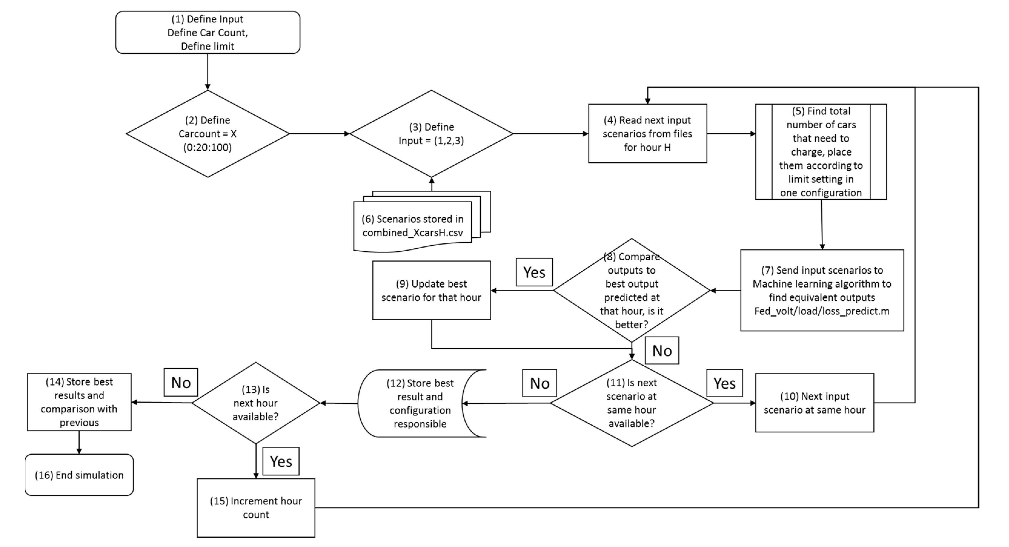
- The flowchart for this method is specified as in Figure 2:
The values for carcount are varied between 0 and 100 in increments of 20. Input, as defined in block 3, refers to 1: line loading, 2: voltage drop and 3: line losses optimization functions respectively. The functions are called accordingly in block 7, which is done via the code files “machinelearning_X.m”, where X can refer to loading, volts or losses. These files also contain the code snippets responsible for comparing the outputs from block 7 with best recorded outputs at that hour, which are later stored in block 14. This is achieved by storing the input configuration corresponding to the least costly output observed when the relevant neural network is called.
The code files mentioned above are called by a consolidated code file called “readjust.m”, which takes into account the input, car count and limit variables and varies the input configuration to call the “machinelearning_X.m” sequence of files accordingly.
Author Contributions
Literature search, S.H.; data curation and creation, S.H.; methodology design, S.H. and P.S.; data validation, S.H.; simulation and results consolidation, S.H.; Supervision, P.S.; revisions and proofreading, P.S. All authors have read and agreed to the published version of the manuscript.
Funding
This research was made possible by the funding provided by the Boysen–TU Dresden Research Training Group.
Conflicts of Interest
The authors declare no conflict of interest.
References
- Pflugradt, N.; Muntwyler, U. Using Behavior Simulation to Synthesize Electromobility Charging Profiles. Available online: http://proceedings.ises.org/paper/eurosun2018/eurosun2018-0161-Pflugradt.pdf (accessed on 11 September 2020).
- Pflugradt, N.; Muntwyler, U. Synthesizing residential load profiles using behavior simulation. Energy Procedia 2017, 122, 655–660. [Google Scholar] [CrossRef]
- Matlab Documentation. Available online: https://www.mathworks.com/help/matlab/ (accessed on 29 October 2020).
- Schäuble, J.; Kaschub, T.; Ensslen, A.; Jochem, P.; Fichtner, W. Generating electric vehicle load profiles from empirical data of three EV fleets in Southwest Germany. J. Clean. Prod. 2017, 150, 253–266. [Google Scholar] [CrossRef] [Green Version]
- Ensslen, A.; Jochem, J.; Schäuble, J.; Babrowski, S.; Fichtner, W. User Acceptance of Electric Vehicles in the French-German Transnational Context: Results out of the french-german fleet test cross-border mobility for electric vehicles (CROME). In Proceedings of the 13th WCTR, Rio de Jeneiro, Brazil, 15–18 July 2013. [Google Scholar]
- Strunz, K.; Abbasi, E.; Abbey, C.; Andrieu, C.; Gao, F.; Gaunt, T.; Iravani, R. Benchmark Systems for Network Integration of Renewable and Distributed Energy Resources; CIGRE: Paris, France, 2009. [Google Scholar]
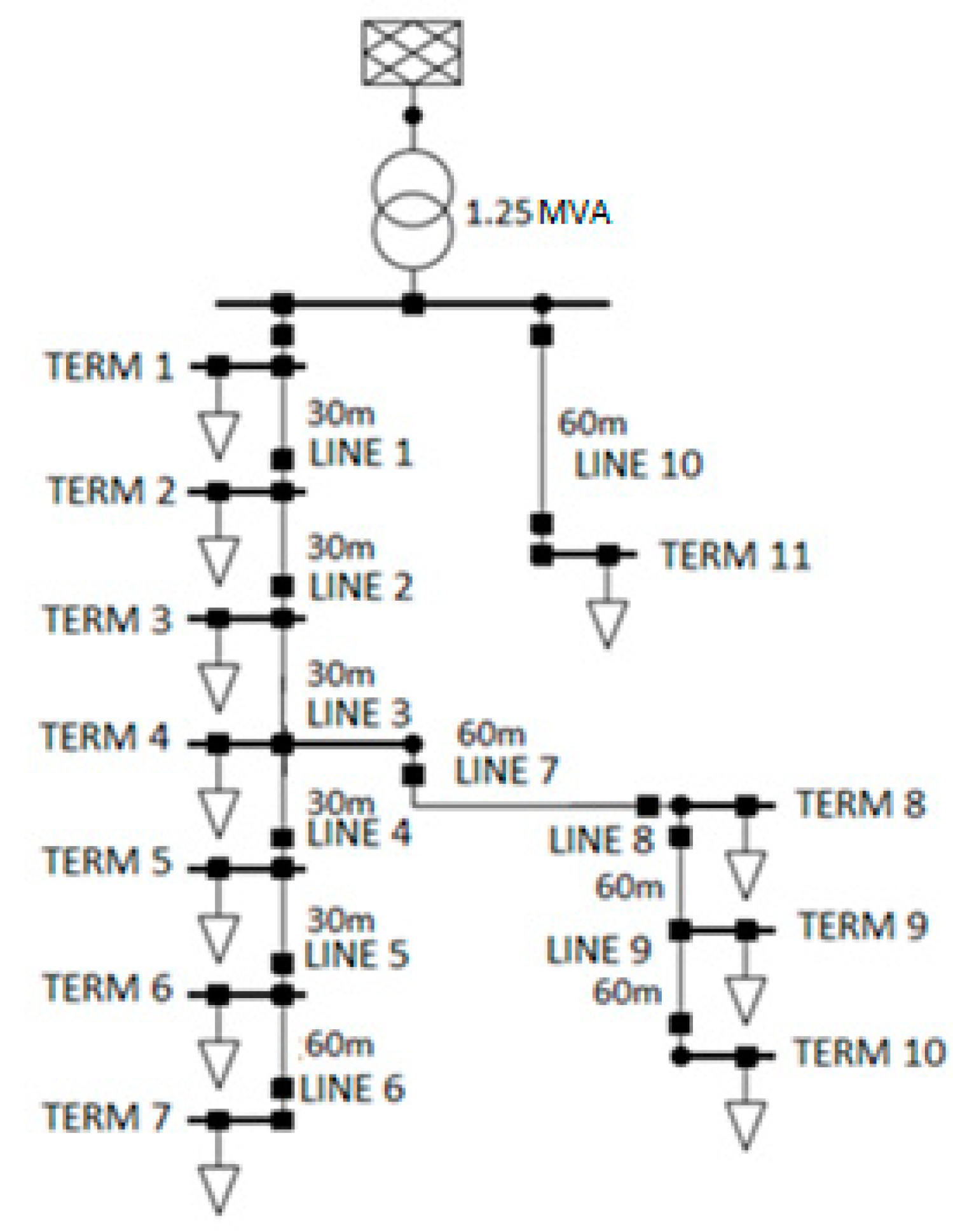
Figure 1.
Grid model [6].
Figure 1.
Grid model [6].

Figure 2.
Scenario creation process.


Table 1.
Network line parameters.
| Name | Cross Sectional Area (mm2) | Length (m) | Rated Current (A) | Z1 (Ohm/Ω) | Phase Angle Z1 (deg/°) | Model Name in Catalog |
|---|---|---|---|---|---|---|
| Line (1) | 240 | 30 | 400 | 0.00433 | 28.63 | 3 × 240 RM 0.6/1 kV |
| Line (2) | 240 | 30 | 400 | 0.00433 | 28.63 | 3 × 240 RM 0.6/1 kV |
| Line (3) | 240 | 30 | 400 | 0.00433 | 28.63 | 3 × 240 RM 0.6/1 kV |
| Line (4) | 150 | 30 | 300 | 0.00655 | 18.46 | 3 × 150 RM 0.6/1 kV |
| Line (5) | 150 | 30 | 300 | 0.00655 | 18.46 | 3 × 150 RM 0.6/1 kV |
| Line (6) | 150 | 60 | 300 | 0.01309 | 18.46 | 3 × 150 RM 0.6/1 kV |
| Line (7) | 150 | 60 | 300 | 0.01309 | 18.46 | 3 × 150 RM 0.6/1 kV |
| Line (8) | 150 | 60 | 300 | 0.01309 | 18.46 | 3 × 150 RM 0.6/1 kV |
| Line (9) | 150 | 60 | 300 | 0.01309 | 18.46 | 3 × 150 RM 0.6/1 kV |
| Line (10) | 240 | 60 | 300 | 0.00865 | 28.63 | 3 × 240 RM 0.6/1 kV |
Table 2.
Consumption demographics.
| Load Name | Active Power (MW) | Reactive Power (MVAR) | Power Factor | Type of Occupant | Employment Status | Child |
|---|---|---|---|---|---|---|
| ld1 | 0.039 | 0.0625 | 0.5305 | Single | Employed | No |
| ld2 | 0.0683 | 0.0171 | 0.9701 | Single | Employed | No |
| ld3 | 0.039 | 0.011 | 0.9626 | Single | Employed | No |
| ld4 | 0.1172 | 0.0147 | 0.9922 | Single | Unemployed | No |
| ld5 | 0.1172 | 0.0436 | 0.9372 | Couple | One Employed | No |
| ld6 | 0.0971 | 0.0523 | 0.8816 | Couple | Both Employed | Yes |
| ld7 | 0.0391 | 0.0087 | 0.976 | Couple | Unemployed | No |
| ld8 | 0.0391 | 0.0087 | 0.976 | Couple | One Employed | Yes |
| ld9 | 0.0879 | 0.0087 | 0.9951 | Multigenerational | Variable | Yes |
| ld10 | 0.0684 | 0.0046 | 0.9976 | Office | ||
| ld11 | 0.0684 | 0.0162 | 0.973 | Office | ||
Publisher’s Note: MDPI stays neutral with regard to jurisdictional claims in published maps and institutional affiliations. |
© 2020 by the authors. Licensee MDPI, Basel, Switzerland. This article is an open access article distributed under the terms and conditions of the Creative Commons Attribution (CC BY) license (http://creativecommons.org/licenses/by/4.0/).
Share and Cite
MDPI and ACS Style
Haider, S.; Schegner, P. Data for Heuristic Optimization of Electric Vehicles’ Charging Configuration Based on Loading Parameters. Data 2020, 5, 102. https://doi.org/10.3390/data5040102
AMA Style
Haider S, Schegner P. Data for Heuristic Optimization of Electric Vehicles’ Charging Configuration Based on Loading Parameters. Data. 2020; 5(4):102. https://doi.org/10.3390/data5040102
Chicago/Turabian StyleHaider, Sajjad, and Peter Schegner. 2020. "Data for Heuristic Optimization of Electric Vehicles’ Charging Configuration Based on Loading Parameters" Data 5, no. 4: 102. https://doi.org/10.3390/data5040102