
Genetic Diversity of Hatchery-Bred Brown Trout (Salmo trutta) Compared with the Wild Population: Potential Effects of Stocking on the Indigenous Gene Pool of a Norwegian Reservoir


Abstract
:1. Introduction
2. Methods
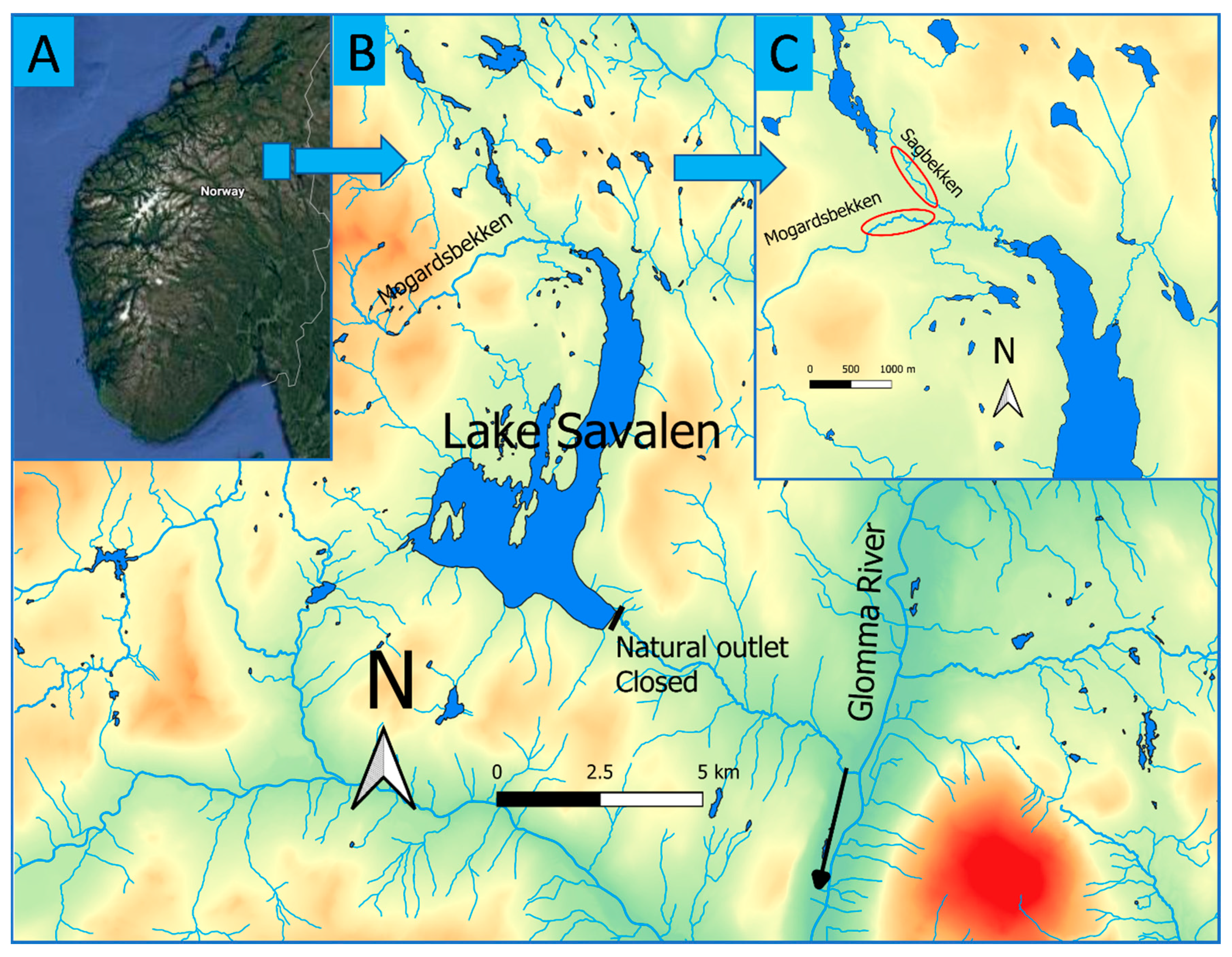
2.1. Study Site
2.2. Sampling
2.3. Genetic Analysis
2.4. Data Analyses
3. Results and Discussion
3.1. Genetic Diversity
3.2. Effective Population Size Ne, Kinship and Selective Mortality
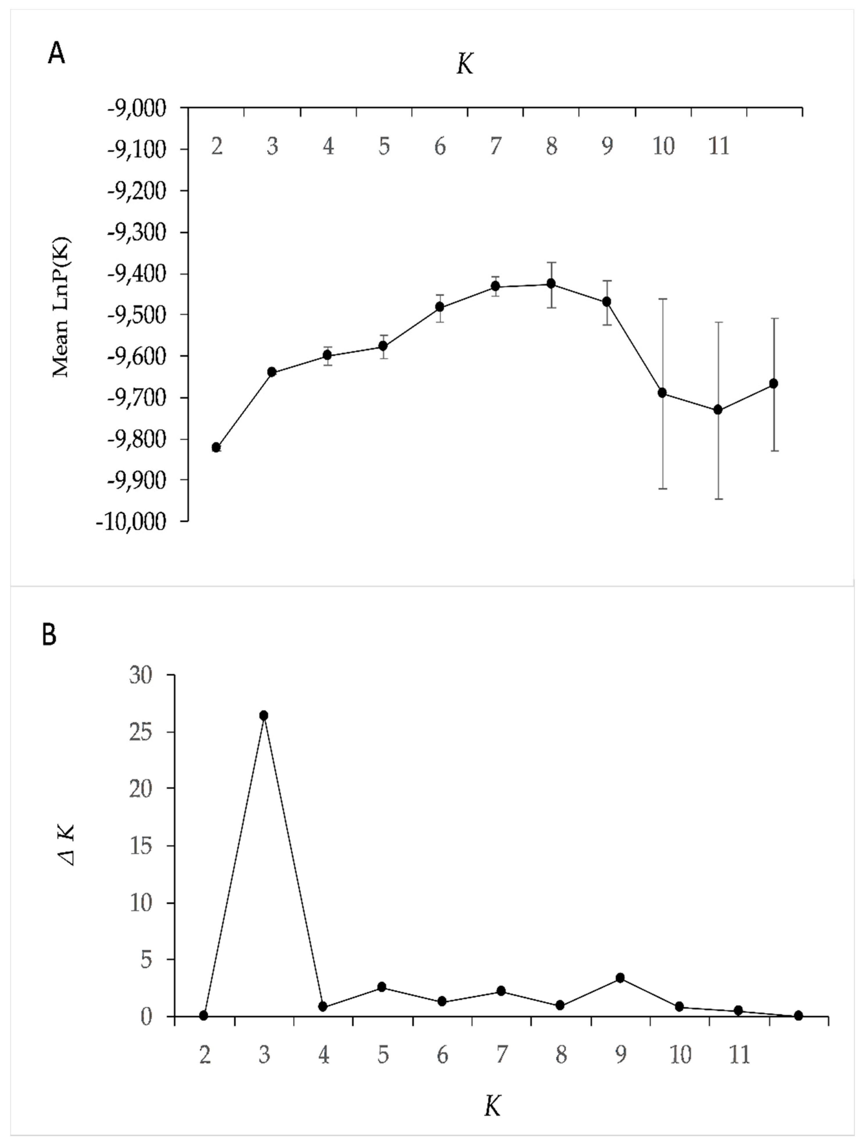
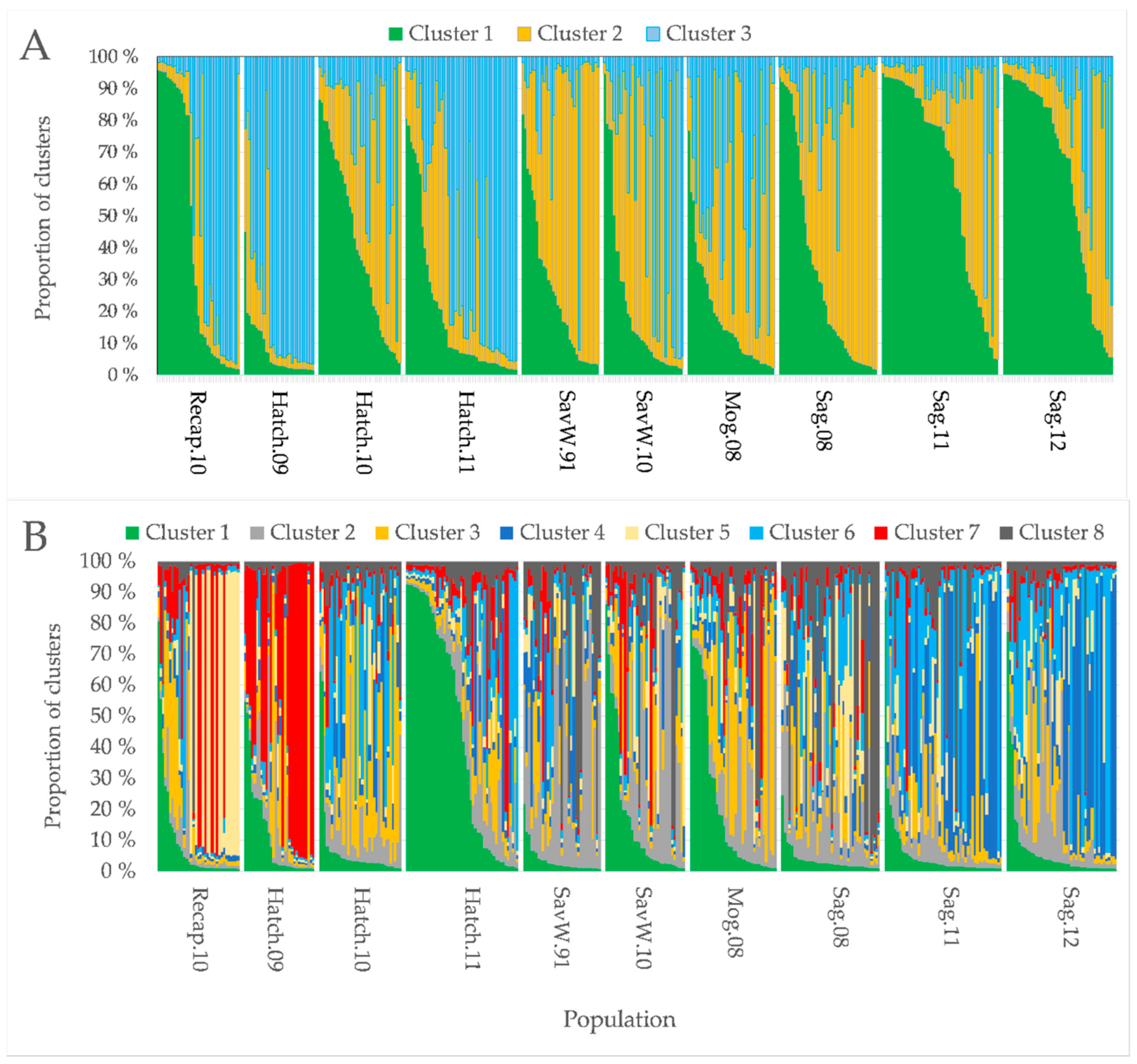
3.3. Genetic Structure
4. Conclusions
Supplementary Materials
Author Contributions
Funding
Institutional Review Board Statement
Data Availability Statement
Acknowledgments
Conflicts of Interest
References
- Cowx, I.G. Stocking strategies. Fish. Manag. Ecol. 1994, 1, 15–30. [Google Scholar] [CrossRef]
- Araki, H.; Berejikian, B.A.; Ford, M.J.; Blouin, M.S. Fitness of hatchery-reared salmonids in the wild. Evol. Appl. 2008, 1, 342–355. [Google Scholar] [CrossRef]
- Pinter, K.; Weiss, S.; Lautsch, E.; Unfer, G. Survival and growth of hatchery and wild brown trout (Salmo trutta) parr in three Austrian headwater streams. Ecol. Freshw. Fish. 2018, 27, 146–157. [Google Scholar] [CrossRef]
- Wills, T.C. Comparative Abundance, Survival, and Growth of One Wild and Two Domestic Brown Trout Strains Stocked in Michigan Rivers. N. Am. J. Fish. Manag. 2006, 26, 535–544. [Google Scholar] [CrossRef]
- Wollebaek, J.; Heggenes, J.; Røed, K.H.; Wollebæk, J. Disentangling stocking introgression and natural migration in brown trout: Survival success and recruitment failure in populations with semi-supportive breeding. Freshw. Biol. 2010, 55, 2626–2638. [Google Scholar] [CrossRef]
- Araki, H.; Cooper, B.; Blouin, M.S. Genetic Effects of Captive Breeding Cause a Rapid, Cumulative Fitness Decline in the Wild. Science 2007, 318, 100–103. [Google Scholar] [CrossRef] [PubMed] [Green Version]
- Bert, T.M.; Crawford, C.R.; Tringali, M.D.; Seyoum, S.; Galvin, J.L.; Higham, M.; Lund, C. Genetic Management of Hatchery-Based Stock Enhancement. In Ecological and Genetic Implications of Aquaculture Activities; Bert, T.M., Ed.; Springer: Dordrecht, The Netherlands, 2007; pp. 123–174. [Google Scholar]
- Linløkken, A.N.; Haugen, T.O.; Kent, M.P.; Lien, S. Genetic differences between wild and hatchery-bred brown trout (Salmo trutta L.) in single nucleotide polymorphisms linked to selective traits. Ecol. Evol. 2017, 7, 4963–4972. [Google Scholar] [CrossRef] [Green Version]
- Jonssonn, S.; Brønnøs, E.; Lundqvist, H. Stocking of brown trout, Salmo trutta L.: Effects of acclimatization. Fish. Manag. Ecol. 1999, 6, 459–473. [Google Scholar] [CrossRef]
- Eckmann, R.; Kugler, M.; Ruhle, C. Evaluating the success of large-scale whitefish stocking at Lake Constance. Adv. Limnol. 2007, 60, 361–368. [Google Scholar]
- Berg, S.; Jorgensen, J. Stocking experiments with 0 + and 1 + trout parr, Salmo trutta L., of wild and hatchery origin: 1. Post-stocking mortality and smolt yield. J. Fish. Biol. 1991, 39, 151–169. [Google Scholar] [CrossRef]
- Hyvarinen, P.; Vehanen, T. Effect of brown trout body size on post-stocking survival and pike predation. Ecol. Freshw. Fish. 2004, 13, 77–84. [Google Scholar] [CrossRef]
- Harbicht, A.; Wilson, C.; Fraser, D.J. Does human-induced hybridization have long-term genetic effects? Empirical testing with domesticated, wild and hybridized fish populations. Evol. Appl. 2014, 7, 1180–1191. [Google Scholar] [CrossRef] [PubMed]
- Ferguson, A. Genetic Impacts of Stocking on Indigenous Brown Trout Populations, in Using Science to Create a Better Place; Environment Agency: Bristol, UK, 2007; p. 93.
- Saint-Pé, K.; Blanchet, S.; Tissot, L.; Poulet, N.; Plasseraud, O.; Loot, G.; Veyssière, C.; Prunier, J.G. Genetic admixture between captive-bred and wild individuals affects patterns of dispersal in a brown trout (Salmo trutta) population. Conserv. Genet. 2018, 19, 1269–1279. [Google Scholar] [CrossRef] [Green Version]
- Borgstrøm, R. Fiskeribiologiske Undersøkelser i Savalen 1969 og 1970; Laboratorium for Ferskvannsøkologi og Innlandsfiske ved Zoologisk Museum, Universitetet i Oslo: Oslo, Norway, 1971; p. 56. [Google Scholar]
- Johnsen, S.I.; Kraabøl, M.; Sandlund, O.T.; Rognerud, S.; Linløkken, A.; Wærvågen, S.B.; Dokk, J.G. Fiskesamfunnet i Savalen, Alvdal og Tynset Kommuner. Betydningen av Reguleringsinngrep, Beskatning og Avbøtende Tiltak; Norwegian Institute of Nature Research: Trondheim, Norway, 2010; p. 56. [Google Scholar]
- Linløkken, A.N. Fiskeundersøkelser i Savalen, Alvdal og Tynset Kommuner 1990–1991. In Glommaprosjektet Rapport nr. 11. 1993; Hedmark Distriktshøgskole: Hamar, Norway, 1993; p. 29. [Google Scholar]
- Dervo, B.K.; Hegge, O.; Hessen, D.O.; Skurdal, J. Diel food selection of pelagic Arctic charr, Salvelinus alpinus (L.), and brown trout, Salmo trutta L.; in Lake Atnsjo, SE Norway. J. Fish. Biol. 1991, 38, 199–209. [Google Scholar] [CrossRef]
- Hegge, O.; Dervo, B.K.; Skurdal, J.; Hessen, D.O. Habitat utilization by sympatric arctic charr Salvelinus alpinus L. and brown trout Salmo trutta L. in Lake Atnsjo, south-east Norway. Freshw. Biol. 1989, 22, 143–152. [Google Scholar] [CrossRef]
- Carlsson, J.; Nilsson, J. Population genetic structure of brown trout (Salmo trutta L.) within a northern boreal forest stream. Hereditas 2004, 132, 173–181. [Google Scholar] [CrossRef]
- Östergren, J.; Nilsson, J. Importance of life-history and landscape characteristics for genetic structure and genetic diversity of brown trout (Salmo trutta L.). Ecol. Freshw. Fish. 2011, 21, 119–133. [Google Scholar] [CrossRef]
- Hansen, M.M.; Nielsen, E.E.; Mensberg, K.-L.D. The problem of sampling families rather than populations: Relatedness among individuals in samples of juvenile brown trout Salmo trutta L. Mol. Ecol. 1997, 6, 469–474. [Google Scholar] [CrossRef]
- Jonsson, B.; Jonsson, N. Age and Growth in Ecology of Atlantic salmon and Brown Trout; Lorenzen, K., Ed.; Springer: Dordrecht, The Netherlands, 2011; p. 708. [Google Scholar]
- Kumar, R.; Singh, P.J.; Nagpure, N.S.; Kushwaha, B.; Srivastava, S.K.; Lakra, W.S. A non-invasive technique for rapid extraction of DNA from fish scales. Indian J. Exp. Boil. 2007, 45, 992–997. [Google Scholar]
- O’Reilly, P.T.; Hamilton, L.C.; McConnell, S.K.; Wright, J.M. Rapid analysis of genetic variation in Atlantic salmon (Salmo salar) by PCR multiplexing of dinucleotide and tetranucleotide microsatellites. Can. J. Fish. Aquat. Sci. 1996, 53, 2292–2298. [Google Scholar] [CrossRef]
- King, T.L.; Eackles, M.S.; Letcher, B.H. Microsatellite DNA markers for the study of Atlantic salmon (Salmo salar) kinship, population structure, and mixed-fishery analyses. Mol. Ecol. Notes 2005, 5, 130–132. [Google Scholar] [CrossRef]
- Nikolic, N.; Fève, K.; Chevalet, C.; Høyheim, B.; Riquet, J. A set of 37 microsatellite DNA markers for genetic diversity and structure analysis of Atlantic salmon Salmo salar populations. J. Fish. Biol. 2009, 74, 458–466. [Google Scholar] [CrossRef] [PubMed]
- Estoup, A.; Presa, P.; Krieg, F.; Vaiman, D.; Guyomard, R. (CT)n and (GT)n microsatellites: A new class of genetic markers for Salmo trutta L. (brown trout). Heredity 1993, 71, 488–496. [Google Scholar] [CrossRef] [PubMed] [Green Version]
- Glaubitz, J.C. Convert: A user-friendly program to reformat diploid genotypic data for commonly used population genetic software packages. Mol. Ecol. Notes 2004, 4, 309–310. [Google Scholar] [CrossRef]
- Lischer, H.E.L.; Excoffier, L. PGDSpider: An automated data conversion tool for connecting population genetics and genomics programs. Bioinformatics 2011, 28, 298–299. [Google Scholar] [CrossRef] [PubMed] [Green Version]
- Kalinowski, S.T. HP-Rare: A computer program performing rarefaction on measures of allelic diversity. Mol. Ecol. Notes 2005, 5, 187–189. [Google Scholar] [CrossRef]
- Excoffier, L.; Lischer, H.E.L. Arlequin suite ver 3.5: A new series of programs to perform population genetics analyses under Linux and Windows. Mol. Ecol. Resour. 2010, 10, 564–567. [Google Scholar] [CrossRef]
- Rousset, F. GENEPOP’007: A complete re-implementation of the genepop software for Windows and Linux. Mol. Ecol. Resour. 2008, 8, 103–106. [Google Scholar] [CrossRef]
- Do, C.; Waples, R.S.; Peel, D.; Macbeth, G.M.; Tillett, B.J.; Ovenden, J.R. NeEstimator V2: Re-implementation of software for the estimation of contemporary effective population size (Ne) from genetic data. Mol. Ecol. Resour. 2014, 14, 209–214. [Google Scholar] [CrossRef]
- Bartley, D.; Bagley, M.; Gall, G.; Bentley, B. Use of Linkage Disequilibrium Data to Estimate Effective Size of Hatchery and Natural Fish Populations. Conserv. Biol. 1992, 6, 365–375. [Google Scholar] [CrossRef]
- Waples, R.S.; Do, C. Linkage disequilibrium estimates of contemporary Ne using highly variable genetic markers: A largely untapped resource for applied conservation and evolution. Evol. Appl. 2010, 3, 244–262. [Google Scholar] [CrossRef] [PubMed]
- Kalinowski, S.T.; Wagner, A.P.; Taper, M.L. ML-relate: A computer program for maximum likelihood estimation of relatedness and relationship. Mol. Ecol. Notes 2006, 6, 576–579. [Google Scholar] [CrossRef]
- Cornuet, J.M.; Luikart, G. Description and Power Analysis of Two Tests for Detecting Recent Population Bottlenecks From Allele Frequency Data. Genetic 1996, 144, 2001–2014. [Google Scholar] [CrossRef]
- Garza, J.C.; Williamson, E.G. Detection of reduction in population size using data from microsatellite loci. Mol. Ecol. 2001, 10, 305–318. [Google Scholar] [CrossRef]
- Foll, M.; Gaggiotti, O.E. A Genome-Scan Method to Identify Selected Loci Appropriate for Both Dominant and Codominant Markers: A Bayesian Perspective. Genetic 2008, 180, 977–993. [Google Scholar] [CrossRef] [Green Version]
- Foll, M. BayeScan v2.1 User Manual; Laboratoire d’Ecologie Alpine: Grenoble, France, 2012; p. 10. [Google Scholar]
- Pritchard, J.K.; Stephens, M.; Donnelly, P. Inference of Population Structure Using Multilocus Genotype Data. Genetics 2000, 155, 945–959. [Google Scholar] [CrossRef]
- Evanno, G.; Regnaut, S.; Goudet, J. Detecting the number of clusters of individuals using the software structure: A simulation study. Mol. Ecol. 2005, 14, 2611–2620. [Google Scholar] [CrossRef] [Green Version]
- Earl, D.A.; Vonholdt, B.M. STRUCTURE HARVESTER: A website and program for visualizing STRUCTURE output and implementing the Evanno method. Conserv. Genet. Resour. 2012, 4, 359–361. [Google Scholar] [CrossRef]
- Jakobsson, M.; Rosenberg, N.A. CLUMPP: A cluster matching and permutation program for dealing with label switching and multimodality in analysis of population structure. Bioinformatics 2007, 23, 1801–1806. [Google Scholar] [CrossRef] [Green Version]
- Peakall, R.; Smouse, P.E. GenAlEx 6: Genetic analysis in Excel. Population genetic software for teaching and research. Mol. Ecol. Notes 2006, 6, 288–295. [Google Scholar] [CrossRef]
- Maguire, T.L.; Peakall, R.; Saenger, P. Comparative analysis of genetic diversity in the mangrove species Avicennia marina (Forsk.) Vierh. (Avicenniaceae) detected by AFLPs and SSRs. Theor. Appl. Genet. 2002, 104, 388–398. [Google Scholar] [CrossRef] [PubMed]
- Michalakis, Y.; Excoffier, L. A generic estimation of population subdivision using distances between alleles with special reference for microsatellite loci. Genetics 1996, 142, 1061–1064. [Google Scholar] [CrossRef] [PubMed]
- Peakall, R.; Smouse, P.E.; Huff, D.R. Evolutionary implications of allozyme and RAPD variation in diploid populations of dioecious buffalograss Buchloë dactyloides. Mol. Ecol. 1995, 4, 135–148. [Google Scholar] [CrossRef]
- Wahlund, S. Zusammensetzung von populationen and korrelationserscheinungen vom standpunkt der vererbungslehre ausbetrachtet. Hereditas 1928, 11, 65–106. [Google Scholar] [CrossRef]
- Nei, M. F-statistics and analysis of gene diversity in subdivided populations. Ann. Hum. Genet. 1977, 41, 225–233. [Google Scholar] [CrossRef] [PubMed]
- Waples, R.S.; Antao, T.; Luikart, G. Effects of Overlapping Generations on Linkage Disequilibrium Estimates of Effective Population Size. Genetics 2014, 197, 769–780. [Google Scholar] [CrossRef] [Green Version]
- Linløkken, A.N.; Johansen, W.; Wilson, R. Genetic structure of brown trout, Salmo trutta, populations from differently sized tributaries of Lake Mjøsa in south-east Norway. Fish. Manag. Ecol. 2014, 21, 515–525. [Google Scholar] [CrossRef]
- Franklin, I.R. Evolutionary change in small populations. Conservation biology: An evolutionary-ecological perspective. In Conservation Biology: An Evolutionary-Ecological Perspective; Wilcox, M.E.S.B., Ed.; Sinauer Associates: Sunderland, MA, USA, 1980; pp. 135–149. [Google Scholar]
- Frankham, R.; Bradshaw, C.J.A.; Brook, B.W. Genetics in conservation management: Revised recommendations for the 50/500 rules, Red List criteria and population viability analyses. Biol. Conserv. 2014, 170, 56–63. [Google Scholar] [CrossRef]
- Franklin, I.R.; Allendorf, F.W. The 50/500 rule is still valin—Reply to Frankham et al. Letter to Editor. Biol. Conserv. 2014, 176, 284–285. [Google Scholar] [CrossRef]
- Christie, M.R.; Marine, M.L.; French, R.A.; Waples, R.S.; Blouin, M.S. Effective size of a wild salmonid population is greatly reduced by hatchery supplementation. Heredity 2012, 109, 254–260. [Google Scholar] [CrossRef] [Green Version]
- Gossieaux, P.; Bernatchez, L.; Sirois, P.; Garant, D. Impacts of stocking and its intensity on effective population size in Brook Charr (Salvelinus fontinalis) populations. Conserv. Genet. 2019, 20, 729–742. [Google Scholar] [CrossRef]
- Nock, C.; Ovenden, J.R.; Butler, G.; Wooden, I.; Moore, A.; Baverstock, P.R. Population structure, effective population size and adverse effects of stocking in the endangered Australian eastern freshwater cod Maccullochella ikei. J. Fish. Biol. 2011, 78, 303–321. [Google Scholar] [CrossRef] [PubMed]
- Ågren, A.; Vainikka, A.; Janhunen, M.; Hyvärinen, P.; Piironen, J.; Kortet, R. Experimental crossbreeding reveals strain-specific variation in mortality, growth and personality in the brown trout (Salmo trutta). Sci. Rep. 2019, 9, 2771. [Google Scholar] [CrossRef] [PubMed] [Green Version]


| Sample | N | AL | Ar | AP | HO | HE | Ne | FIS | Siblings |
|---|---|---|---|---|---|---|---|---|---|
| Recap.10 | 35 | 5.3 | 4.71 | 0 | 0.75 * | 0.70 | 8.4 (5.3–12.1) | −0.065 | 11.6/8.7% |
| Hatch.09 | 30 | 5.0 | 4.57 | 0 | 0.71 | 0.68 | 10.5 (6.8–16.4) | −0.024 | 3.9/11.7% |
| Hatch.10 | 35 | 6.1 | 5.20 | 0 | 0.68 * | 0.67 | 19.9 (13.6–30.7) | −0.043 | 6.2/9.5% |
| Hatch.11 | 50 | 6.3 | 5.10 | 0 | 0.75 * | 0.73 | 18.7 (14.0–25.2) | 0.016 | 5.4/9.1% |
| Pooled hatch.09–11 | 113 | 7.4 | 5.34 | 0 | 0.62 * | 0.63 | 33.0 (26.9–40.9) | −0.003 | 3.4/13.4% |
| Mean of subsamples | 35 | 6.4 | 5.40 | 0 | 0.61 | 0.63 | 28.7 (19.4–38.0) | 0.014 | 3.4/11.0% |
| SavW.91 | 33 | 8.0 | 6.73 | 5 | 0.71 | 0.77 | 481.0 (85.1–inf.) | 0.065 | 1.5/12.1% |
| SavW.10 | 34 | 7.9 | 6.53 | 2 | 0.74 * | 0.77 | 103.4 (50.4–938.6) | 0.071 | 1.8/13.9% |
| Mog.08 | 37 | 6.6 | 5.67 | 3 | 0.70 * | 0.75 | 39.5 (25.3–72.0) | 0.124 * | 2.4/14.1% |
| Sag.08 | 42 | 7.0 | 5.92 | 0 | 0.76 * | 0.75 | 38.4 (26.4–61.3) | −0.044 | 3.8/12.3% |
| Sag.11 | 50 | 6.0 | 5.08 | 0 | 0.69 | 0.67 | 43.3 (28.6–73.9) | −0.010 | 3.8/11.5% |
| Sag.12 | 47 | 6.8 | 5.46 | 0 | 0.77 * | 0.72 | 45.8 (30.5–78.2) | −0.100 | 4.3/13.0% |
| Wilcoxon Test H Excess p-Values | Garza–Williamson Index | ||||
|---|---|---|---|---|---|
| Sample | I.A.M. | T.P.M. | S.M.M. | Unmodified | Modified |
| 1. Recap.10 | 0.002 | 0.002 | 0.230 | 0.435 | 0.345 (7) |
| 2. Hatch.09 | 0.002 | 0.004 | 0.273 | 0.432 | 0.322 (7) |
| 3. Hatch.10 | 0.020 | 0.473 | 0.981 | 0.496 | 0.383 (7) |
| 4. Hatch.11 | 0.004 | 0.012 | 0.578 | 0.488 | 0.375 (7) |
| 5. SavW.91 | 0.002 | 0.191 | 0.770 | 0.523 | 0.389 (6) |
| 6. SavW.10 | 0.004 | 0.156 | 0.081 | 0.477 | 0.471 (6) |
| 7. Mog.08 | 0.001 | 0.021 | 0.434 | 0.519 | 0.400 (7) |
| 8. Sag.08 | 0.002 | 0.020 | 0.680 | 0.463 | 0.437 (6) |
| 9. Sag.11 | 0.018 | 0.232 | 0.010 | 0.479 | 0.393 (6) |
| 10. Sag.12 | 0.006 | 0.126 | 0.963 | 0.455 | 0.425 |
| Group Tested | Locus | PO | Prob. | log10(PO) | q Value | Alpha | FST |
|---|---|---|---|---|---|---|---|
| Recap.10+ | SSa197 | 20.0 | 0.952 | 1.301 | 0.885 | −0.961 | 0.055 |
| Hatch.09+ | SSaD170 | >> | 1.000 | 1000 | 0.920 | −1.327 | 0.039 |
| Hatch.10+ | SSaD190 | 7.0 | 0.875 | 0.843 | 0.863 | −0.804 | 0.063 |
| Hatch.11+ | SSaD71 | 624 | 0.998 | 2.795 | 0.925 | −1.152 | 0.046 |
| SavW.91+ | SSaD85 | 2499 | 1.000 | 3.398 | 0.907 | −1.148 | 0.046 |
| SavW.10+ | Brun13 | 0.64 | 0.391 | −0.192 | 0.914 | −0.274 | 0.099 |
| Mog.08+ | SSa85 | 33.7 | 0.971 | 1.528 | 0.898 | −1.150 | 0.048 |
| Sag.08+ | STR73I | >> | 1.000 | 1000 | 0.799 | −1.740 | 0.028 |
| Sag.11+ | |||||||
| Sag.12 | |||||||
| Hatch.09+ | SSa197 | 0.08 | 0.070 | −1.125 | 0.916 | −0.033 | 0.078 |
| Hatch.10+ | SSaD170 | 0.05 | 0.051 | −1.268 | 0.932 | −0.011 | 0.079 |
| Hatch.11 | SSaD190 | 0.11 | 0.099 | −0.958 | 0.901 | −0.066 | 0.076 |
| SSaD71 | 0.06 | 0.053 | −1.252 | 0.926 | 0.001 | 0.080 | |
| SSaD85 | 0.06 | 0.053 | −1.249 | 0.922 | −0.008 | 0.079 | |
| Brun13 | 0.05 | 0.052 | −1.263 | 0.929 | 0.013 | 0.081 | |
| SSa85 | 0.08 | 0.070 | −1.123 | 0.911 | −0.025 | 0.078 | |
| STR73I | 0.11 | 0.099 | −0.961 | 0.901 | −0.055 | 0.077 | |
| Recap.10+ | SSa197 | 0.08 | 0.071 | −1.115 | 0.885 | −0.032 | 0.076 |
| Hatch.09+ | SSaD170 | 0.05 | 0.046 | −1.319 | 0.920 | −0.012 | 0.077 |
| Hatch.10+ | SSaD190 | 0.08 | 0.072 | −1.111 | 0.863 | −0.036 | 0.076 |
| Hatch.11 | SSaD71 | 0.04 | 0.043 | −1.352 | 0.925 | 0.002 | 0.078 |
| SSaD85 | 0.06 | 0.054 | −1.240 | 0.907 | −0.013 | 0.077 | |
| Brun13 | 0.06 | 0.052 | −1.259 | 0.914 | 0.014 | 0.079 | |
| SSa85 | 0.07 | 0.064 | −1.164 | 0.898 | −0.027 | 0.077 | |
| STR73I | 0.25 | 0.201 | −0.599 | 0.799 | −0.219 | 0.069 | |
| SavW.91+ | SSa197 | 0.43 | 0.298 | −0.372 | 0.316 | −0.260 | 0.048 |
| SavW.10+ | SSaD170 | 1250 | 0.999 | 3.097 | 0.001 | −1.327 | 0.018 |
| Mog.08+ | SSaD190 | 1.26 | 0.557 | 0.100 | 0.197 | −0.529 | 0.038 |
| Sag.08+ | SSaD71 | 3.34 | 0.769 | 0.523 | 0.136 | −0.836 | 0.029 |
| Sag.11+ | SSaD85 | 6.16 | 0.860 | 0.790 | 0.070 | −0.877 | 0.028 |
| Sag.12 | Brun13 | 0.04 | 0.040 | −1.378 | 0.397 | −0.002 | 0.060 |
| SSa85 | 4.78 | 0.827 | 0.679 | 0.104 | −1.049 | 0.025 | |
| STR73I | 0.91 | 0.476 | −0.042 | 0.252 | −0.617 | 0.039 | |
| Recap.10+ | SSa197 | 2.48 | 0.713 | 0.394 | 0.103 | −0.686 | 0.048 |
| SavW.91+ | SSaD170 | 2500 | 1.000 | 3.398 | 0.000 | −1.242 | 0.028 |
| SavW.10+ | SSaD190 | 0.93 | 0.482 | −0.031 | 0.162 | −0.417 | 0.060 |
| Mog.08+ | SSaD71 | 31.0 | 0.969 | 1.492 | 0.016 | −1.096 | 0.033 |
| Sag.08+ | SSaD85 | 5.59 | 0.848 | 0.748 | 0.066 | −0.799 | 0.043 |
| Sag.11+ | Brun13 | 0.05 | 0.052 | −1.261 | 0.260 | −0.018 | 0.083 |
| Sag.12 | SSa85 | 14.2 | 0.934 | 1.152 | 0.032 | −1.147 | 0.032 |
| STR73I | 11.3 | 0.919 | 1.054 | 0.045 | −1.323 | 0.029 |
| Sample No | ||||||||||
| Sample | No | 1 | 2 | 3 | 4 | 5 | 6 | 7 | 8 | 9 |
| Recap.10 | 1 | - | ||||||||
| Hatch.09 | 2 | 0.051 * | - | |||||||
| Hatch.10 | 3 | 0.036 * | 0.081 * | - | ||||||
| Hatch.11 | 4 | 0.042 * | 0.043 * | 0.047 * | - | |||||
| SavW.91 | 5 | 0.043 * | 0.068 * | 0.033 * | 0.036 * | - | ||||
| SavW.10 | 6 | 0.022 * | 0.045 * | 0.021 * | 0.012 * | 0.008 | - | |||
| Sag.08 | 7 | 0.034 * | 0.061 * | 0.025 * | 0.031 * | 0.005 | 0.003 | - | ||
| Mog.08 | 8 | 0.037 * | 0.051 * | 0.029 * | 0.017 * | 0.024 * | 0.001 | 0.014 * | - | |
| Sag.11 | 9 | 0.059 * | 0.112 * | 0.030 * | 0.051 * | 0.037 * | 0.037 * | 0.033 * | 0.042 * | - |
| Sag.12 | 10 | 0.033 * | 0.078 * | 0.018 * | 0.034 * | 0.017 * | 0.015 * | 0.017 * | 0.024 * | 0.007 * |
Publisher’s Note: MDPI stays neutral with regard to jurisdictional claims in published maps and institutional affiliations. |
© 2021 by the authors. Licensee MDPI, Basel, Switzerland. This article is an open access article distributed under the terms and conditions of the Creative Commons Attribution (CC BY) license (https://creativecommons.org/licenses/by/4.0/).
Share and Cite
Linløkken, A.N.; Johnsen, S.I.; Johansen, W. Genetic Diversity of Hatchery-Bred Brown Trout (Salmo trutta) Compared with the Wild Population: Potential Effects of Stocking on the Indigenous Gene Pool of a Norwegian Reservoir. Diversity 2021, 13, 414. https://doi.org/10.3390/d13090414
Linløkken AN, Johnsen SI, Johansen W. Genetic Diversity of Hatchery-Bred Brown Trout (Salmo trutta) Compared with the Wild Population: Potential Effects of Stocking on the Indigenous Gene Pool of a Norwegian Reservoir. Diversity. 2021; 13(9):414. https://doi.org/10.3390/d13090414
Chicago/Turabian StyleLinløkken, Arne N., Stein I. Johnsen, and Wenche Johansen. 2021. "Genetic Diversity of Hatchery-Bred Brown Trout (Salmo trutta) Compared with the Wild Population: Potential Effects of Stocking on the Indigenous Gene Pool of a Norwegian Reservoir" Diversity 13, no. 9: 414. https://doi.org/10.3390/d13090414