Phylogenetic Signal of Indels and the Neoavian Radiation


1
Department of Biology, New Mexico State University, Las Cruces, NM 88003, USA
2
Department of Biology, University of Florida, Gainesville, FL 32607, USA
3
Electrical and Computer Engineering, University of California, San Diego, CA 92093, USA
*
Authors to whom correspondence should be addressed.
Diversity 2019, 11(7), 108; https://doi.org/10.3390/d11070108
Submission received: 3 June 2019
/
Revised: 3 July 2019
/
Accepted: 4 July 2019
/
Published: 6 July 2019
(This article belongs to the Special Issue Genomic Analyses of Avian Evolution)
Abstract
:The early radiation of Neoaves has been hypothesized to be an intractable “hard polytomy”. We explore the fundamental properties of insertion/deletion alleles (indels), an under-utilized form of genomic data with the potential to help solve this. We scored >5 million indels from >7000 pan-genomic intronic and ultraconserved element (UCE) loci in 48 representatives of all neoavian orders. We found that intronic and UCE indels exhibited less homoplasy than nucleotide (nt) data. Gene trees estimated using indel data were less resolved than those estimated using nt data. Nevertheless, Accurate Species TRee Algorithm (ASTRAL) species trees estimated using indels were generally similar to nt-based ASTRAL trees, albeit with lower support. However, the power of indel gene trees became clear when we combined them with nt gene trees, including a striking result for UCEs. The individual UCE indel and nt ASTRAL trees were incongruent with each other and with the intron ASTRAL trees; however, the combined indel+nt ASTRAL tree was much more congruent with the intronic trees. Finally, combining indel and nt data for both introns and UCEs provided sufficient power to reduce the scope of the polytomy that was previously proposed for several supraordinal lineages of Neoaves.
1. Introduction
There have been many attempts to resolve the relationships among the major lineages of birds using molecular data [1]. The earliest efforts used mitochondrial data (e.g., [2,3,4]), but attention rapidly shifted to the nuclear genome. Analyses of nuclear sequence data began by using individual genes [5,6,7] or small numbers of genes [8,9] with increasingly comprehensive higher-taxon sampling. A constant across all of these studies was the poor resolution of the relationships at the base of the most species-rich avian clade, Neoaves. The absence of resolution was so striking that Poe and Chubb [10] suggested that was evidence of a hard polytomy (simultaneous cladogenic events). Subsequent analyses of multiple genes [11,12,13] provided convincing support for monophyly of several supraordinal bird clades, falsifying the specific version of the hard polytomy hypothesis that was proposed by Poe and Chubb [10]. However, the multigene studies were still unable to provide strong support for all relationships among orders. In fact, subsequent phylogenomic studies using hundreds or even thousands of genes [14,15,16] only provided convincing evidence that a few additional supraordinal clades were monophyletic despite the use of very large data matrices, some comprising as much as 322 megabase pairs (Mbp) of sequence data, for analyses. The continued lack of resolution in the bird tree in the phylogenomic era led Suh [17] to advocate a return to the hard polytomy hypothesis involving the radiation of nine clades at the base of Neoaves (as in Figure 1, excluding Phaethontimorphae).
The hard polytomy hypothesis makes a fundamental prediction that individual gene trees will show no more similarity to each other than expected for random trees generated by the coalescent process. Sayyari and Mirarab [19] proposed a statistical test of the polytomy hypothesis based on quartet frequencies; when they applied this test to the bird tree, they were unable to reject the null hypothesis of a zero-length branch (i.e., a true polytomy) for several branches near the base of Neoaves (Figure 2). Suh [17] combined two lines of evidence when he argued for a hard polytomy at the base of Neoaves. The first line of evidence was the conflict among gene trees and between the gene trees and estimates of the species tree, presumably due to incomplete lineage sorting (ILS). Gene tree incongruence is certainly ubiquitous for the base of Neoaves. Consider, for example, that none of the 14,446 individual gene trees of Jarvis et al. [15] were identical to the estimated species tree. However, the observation that there is extensive conflict among gene trees does not provide direct evidence of a hard polytomy because ILS is expected to be ubiquitous, even for fully resolved species trees. Gene tree–species tree conflicts due to ILS are an inevitable consequence of genetic drift in a set of populations connected by a phylogenetic tree [20,21], although there will be more ILS for short internal branches (like the branches at the base of Neoaves; [15,16]). The hard polytomy hypothesis is only corroborated when quartets within gene trees are considered and the percentage of gene trees that support each of the three mutually exclusive paired sister taxa in a quartet approaches one-third [19]. Of course, the hard polytomy test assumes the estimated gene trees are accurate; any topological errors in the gene trees could inflate the estimated amount of ILS [22].
The second argument Suh [17] used to support the hard polytomy hypothesis is the fact that all available large-scale estimates of avian phylogeny conflict with each other. However, the observed conflicts among phylogenomic estimates of the avian species tree could also reflect errors in phylogenetic estimation [1]. If some of the phylogenomic trees are actually better estimates of the true avian species tree (or parts of it), then the conflicts could reflect errors in the poorer estimates of the tree. Lack of resolution along short branches in gene trees can also result from a paucity of informative characters [26], with relative abundance varying among data partitions according to their inherent mutational rate and selective constraints. Differences in levels of homoplasy and/or systematic bias associated with specific data partitions can contribute to apparent gene tree conflict [1]. Incongruence between relatively accurate estimates of phylogeny and biased estimates of phylogeny do not provide evidence to support the hard polytomy hypothesis. Regardless of the details, it is important to consider the possibility that some (or even all) of the currently available phylogenomic trees for birds simply represent biased estimates of avian phylogeny. Obviously, the quartet-based polytomy test can have both false positive and false negative errors if gene trees are biased in some systematic manner, for example, if one of three possible gene tree quartets is overrepresented due to phenomenon such as long-branch attraction [27]. Ultimately, whether one embraces the hard polytomy hypothesis or views the base of Neoaves as a tree that is likely to be resolved, it is important to consider the possibility that some (or even all) of the currently available phylogenomic trees for birds represent biased estimates of avian phylogeny.
There is certainly evidence that large-scale bird trees based on different data types yield distinct estimates of phylogeny [15,18]. Both Jarvis et al. [15] and Reddy et al. [18] argued that the trees that emerge in analyses of non-coding data might be closer to the true tree. One argument for this hypothesis is the observation that coding data exhibits more variation in base composition [15,18]; this means that coding data are likely to exhibit stronger violations of the assumptions of the general time reversible (GTR) model than non-coding data. However, that argument is indirect. Another way to corroborate the hypothesis that trees generated using non-coding data are closer to the true tree would be to conduct analyses of yet another data type. Insertions and deletions (indels) represent a distinct type of data that has been historically under-utilized in phylogenetics. This reflects, at least in part, the fact that their positions in alignments has been derided as ambiguous or subjective [28,29]; however, that argument is unconvincing because phylogenetic inference using nt data depends on the same alignment used to place indels. Ultimately, questions regarding the utility of indels in phylogenetics are empirical and must be addressed by comparisons to analyses that use nt data. Regardless of the details, the larger point is that phylogenetic analyses of indels might provide a different way of looking at existing data. Assuming that one accepts that indels are useful characters for phylogenetic estimation, then one is left with the question of the best model for their analysis. This leads to a more valid reason why indels have been historically under-utilized in phylogenetics: because, in sharp contrast to the situation for nt substitutions where a plethora of models that are informed by knowledge of substitution processes exist [30], the models that are currently available for indel analysis are few and relatively unsophisticated. Some of the more sophisticated indel models (e.g., the TKF91 and TKF92 [Thorne–Kishino–Felsenstein] models [31,32] and their extensions [33] as well as the “Wagner–Dollo duet” model [34]) are impractical for phylogenomic-scale data sets. This has meant that most analyses of indels have coded them as binary characters [35] that are then analyzed using either the maximum parsimony (MP) criterion or the maximum likelihood (ML) criterion using a simple model [35]. When analyses of indels are conducted, a variant of the two-state Markov model (i.e., Cavender–Farris–Neyman [CFN] model [36,37,38]) that assumes unequal state frequencies and includes among-characters rate heterogeneity is typically used (we used a variant of the CFN model with Γ-distributed rate variation that is called BINGAMMA in Randomized Axelerated Maximum Likelihood (RaxML) [39]). Use of this unsophisticated model could be a problem because indel data from biological sources almost certainly violate the CFN+Γ model. However, it seems reasonable to postulate that analyses based on nts and indels will deviate from the models used from their analysis in different ways. Thus, indel data could provide a different way of looking at the data that is likely to be valuable, despite the relative dearth of models for indel analyses.
Despite the limited number of models available for analyses of indels, there are reasons to be hopeful. It has long been clear that most indel datasets exhibit less homoplasy than nt datasets [7,9,15,35,38]. Their low homoplasy is due, at least in part, to the fact that they have a very large character state space [40]. Evolution is expected to be homoplasy-free when the character state space is large enough [41]. MP should be a consistent estimator of phylogeny when characters reach the limiting condition of being homoplasy-free, and simple ML methods are likely to perform better when characters exhibit limited homoplasy. In addition to the large state space, the limited homoplasy of indels is also likely to reflect the mechanisms responsible for the origin of novel indel mutations and the fixation of those mutations in populations. Those mechanisms differ in fundamental ways from those responsible for nt substitutions. The mutational mechanisms responsible for the origin of new indels include phenomena ranging from replication slippage and unequal crossing over [42,43,44,45]. For the insertion of longer sequences, one finds other processes making substantial contributions, like the insertion of organellar DNA into the nuclear genome as pseudogenes (numts; [46,47,48]) as well as the insertion of transposable elements (TEs) [49,50,51]. Of course, one could postulate that some mutational mechanisms generate unexpectedly large numbers of identical indels or that some types of identical indels have a higher probability of fixation, but this is the equivalent of postulating that indels have a smaller state space than expected given naïve models. We can largely exclude the latter possibility because empirical observations indicate that, as an ensemble, indels exhibit less homoplasy than nt substitutions [7,9,15,35,38] and that long indels exhibit less homoplasy than short ones [9,15] (also see below in Results and Discussion, Section 3.1). The observation of very low homoplasy for long indels might seem to suggest that it is desirable to limit analyses to the largest indels, but there are too few of them to clearly resolve many of the short internodes at the base of Neoaves (Supplemental Materials S.1, Table S1, Figure S1). Fortunately, even the most length-inclusive indel data sets exhibit low homoplasy relative to nts, and indels comprise a very large data set that spans the entire genome (Tables S12 and S13 in Jarvis et al. [15]). Thus, it seems reasonable to investigate whether phylogenomic-scale analyses of indels can shed light on the phylogeny of birds.
Since indel and nt data are likely to deviate from the models used from their analysis in different ways, it is reasonable to postulate that if they converge on a specific topology then that may be indicative of underlying phylogenetic signal. Herein, we analyze a genome-scale indel data matrix for birds, using the CFN+Γ model. We compare the behavior of indels and nts from a common set of genome-scale loci from the full diversity of extant birds at the ordinal level in the context of multispecies coalescent (MSC) analyses, with limited comparison to previously unpublished MP and ML trees (Supplemental Figures S2–S7). We extend prior studies of avian phylogeny that used indel data [38,52] by increasing the data matrix size by almost three orders of magnitude and by implementing methods that explicitly address conflict among gene trees due to the multispecies coalescent.
Herein we address several major questions regarding the properties of indel data as they are applied in phylogenetic analyses of Neoaves. First, how similar are the estimates of gene trees generated by analyses of indels to those based on nt data? To answer this, one must ask how well resolved are indel trees? Are indel and nt gene trees generated from the same loci congruent with one another? Are there differences in the level of performance of indels among different data partitions, and if there are then do partitioned nt data exhibit similar differences? Can nt and indel data be combined in MSC analysis? If so, then do combined data perform better than either alone? Finally, do analyses of two very different sources of phylogenetic information—indels and nt sequence data—provide insights into the hard polytomy hypothesis? We expect the answers to the questions we posed to provide insight into the phylogenetic utility of indels for resolving the avian tree of life and, more generally, to reveal information about the potential for MSC analyses of indel data to be a tool for phylogenomic analyses.
2. Methods
We studied the indels present in the 2516 intronic and 3769 ultraconserved element (UCE) loci from Jarvis et al. [53] datasets. Indels were scored by the principle of simple indel coding [54]. Indels for the MP analyses were scored using 2xread [55,56] and verified using GapCoder [57]. Indels for multispecies coalescent analyses were scored for each locus using 2matrix [56], an updated version of 2xread, in combination with a custom perl script (see Supplemental Material). MP bootstrap (BS) trees were generated using Tree Analysis Technology (TNT) [58] (Figures S2–S5). The retention index (RI; [59]) was calculated and MP trees produced using TNT [58] and PAUP*4.0b11 [60] on ML gene and species trees. Individual introns were concatenated by locus. ML estimates of gene trees were generated using the BINGAMMA model in RAxML version-8.2.11 [39] (Figures S6 and S7).
Coalescent trees were generated using ASTRAL-III [24]. For many analyses, we collapsed poorly supported nodes, which we defined as those with BS support below a specific threshold, to yield polytomies. Sensitivity analyses were performed by varying the level of BS support of input gene trees for ASTRAL analysis from 0–33% contraction. Where we do not specify, our results are based on gene trees with branches of 5% or less BS contracted. The 5% threshold, while somewhat arbitrary, was chosen based on previous simulation and empirical results [24] that indicated only very low values of support should be contracted and that 5% works well for an avian nt dataset. Support values in the low range (e.g., <20%) produce robust results, as we will show. We used DiscoVista [61] to examine quartet frequencies, clade recovery, and Robinson–Foulds (RF) distances. The calculation of local posterior probabilities (localPP) in ASTRAL is described in Sayyari and Mirarab [22]; for ASTRAL analyses that used both nt+indel gene trees for the same locus, we instructed ASTRAL to count each pair of estimated gene trees as one tree (this was done to avoid double counting the same locus twice). Tests of the hard polytomy were performed in ASTRAL as described [19]. Our taxonomic nomenclature generally follows Ericson [62], Yuri et al. [38], Jarvis et al. [15], and Cracraft [63] where it does not conflict with the former two. Whenever possible (i.e., barring supraordinal clades), we use common names because we believe they are easier to read and remember.
Data and code used in this paper can be found in Supplementary Materials.
3. Results and Discussion
Binary coding of indels in the introns and non-coding UCE alignments from Jarvis et al. [53] resulted in an indel data matrix with more than five million characters (Table 1). This was almost three orders of magnitude larger than the Yuri et al. [38] data matrix, which had 12,030 characters and was the largest previous study focused on avian indels. Almost 25% of the indels were parsimony informative (Table 1). Although the number of indel characters is an order of magnitude lower than number of aligned nts, it still represents a very large phylogenetic data matrix. The number of indels per locus varied from a minimum of six to more than 10,000, with the intronic regions typically having more indels per locus than the UCEs (Table 1).
3.1. Indels Exhibit Less Homoplasy Than nt Substitutions
Measured (apparent) homoplasy represents three distinct phenomena that contribute to character state distributions that conflict with an estimate of the species phylogeny. These phenomena are: (1) true homoplasy (convergence, reversal, and parallelism), (2) hemiplasy (characters that are perfectly consistent with their underlying gene tree but conflict with the species tree due to ILS [64]), and (3) analytical errors (e.g., alignment errors). Ensemble RI provides a metric of homoplasy relative to a specific estimate of the species tree, and it includes all three sources of apparent homoplasy (including error introduced by inaccurate estimation of the species tree). As expected, based on prior studies, all indel size classes have lower homoplasy (higher RI) than nt substitutions (nt RI is 0.31 whereas indel RI ranges from 0.49 to 0.86 depending on the indel size class; Table 2). If we focus on the fit of individual indels to an estimate of the species tree, using the percentage of indels with perfect fit to the tree (RI = 1.0), we see a similar size dependence (Figure 3). The number of indels falls off sharply as a function of indel size, probably reflecting the complex mixture of phenomena that lead to the accumulation of indels over evolutionary time. First, mutational origin of indels is heterogeneous, with very small indels reflecting phenomena like replication slippage followed by a shift to unequal crossing-over for somewhat larger indels and finally arriving at the largest size class, that is likely to include many TE insertions. Han et al. [65] examined a set of avian introns and found that 73% of insertions that were >40 bp in length were TE insertions. Second, the probability of indel fixation may differ for indels of different sizes. Regardless of the differences within indels, these data confirm previous work showing that indels are less homoplastic than nt substitutions [35,38] and they are likely to provide a useful source of phylogenetic information.
Hemiplasy is a reflection of the fact that gene and species histories conflict. This leads to a situation where a character (e.g., an indel) may be perfectly consistent with the associated gene tree but it appears to be homoplastic because it is inconsistent with the species tree [64]. Thus, it should be possible to minimize the contribution of hemiplasy to the observed RI by calculating the RI for individually optimized gene trees. There are two potential biases that might emerge when RI is estimated for individual gene trees. First, we have to use estimated gene trees that can have topological errors [66,67]. Second, contiguous genomic segments can be associated with multiple gene trees due to intralocus recombination [67,68]. Thus, indels can exhibit indel hemiplasy even if one focuses on individual genes. More properly, one can see hemiplasy in any region that includes multiple c-genes, where c-genes are defined as DNA segments with a single evolutionary history [69,70]. The common usage of the term “gene” may refer to a DNA segment that includes multiple c-genes (indeed, large gene regions subject to recombination will almost certainly include multiple c-genes). Nevertheless, using estimates of individual gene trees for the RI calculations likely minimize the impact of hemiplasy and therefore provide a more accurate measurement of true homoplasy.
Intronic indels exhibit slightly more homoplasy than UCE indels, even when estimates of individual gene trees were used to calculate the ensemble RI for each gene (ensemble RI: intron indel mean = 0.59, median = 0.57, 1st quartile = 0.51, 3rd quartile = 0.66; UCE indel mean = 0.65, median = 0.65, 1st quartile = 0.60, 3rd quartile = 0.70) (Figure 4). Indels exhibited substantially less homoplasy in both data types than nt substitutions (ensemble RI: intron nt mean = 0.32, median = 0.32, 1st quartile = 0.30, 3rd quartile = 0.34; UCE nt mean = 0.34, median = 0.34, 1st quartile = 0.32, 3rd quartile = 0.36) (Figure 4). The lesser variation of ensemble RI in nt gene trees may be due both to phylogenetic signal and/or covariance of physically and/or selectively linked nt positions. The difference in intron nt vs. indel gene tree ensemble RI is not due to the obvious difference in dataset sizes; the relationship holds up when loci are selected to match indel and nt dataset sizes (Figure S8).
3.2. How Well Resolved Are Indel Trees in Comparison to nt Trees?
Resolution of both intron and UCE nt gene trees is superior to that of indel gene trees. Indel gene trees are less resolved as binary trees than nt gene trees for any cutoff of BS support (contraction), despite differences in resolution between intron and UCE partitions (Figure 5a). With contraction of only branches with 0% support, the median (across loci) number of binary nodes recovered normalized to the maximum possible is 100% for intron nt gene trees, somewhat less for intron indel and UCE nt gene trees, and substantially lower for UCE indel gene trees. The median percentage of recovered nodes drops rapidly and monotonically to below 50% of the maximum possible as nodes are contracted up to 33% based on BS support. UCE gene trees are less resolved than intron gene trees within each data type. The relative differences between data types and partitions remain the same at all levels of contraction. Similarly, mean BS support averaged over all branches of each gene tree is higher for nt gene trees than indel gene trees, despite differences between intron and UCE partitions (Figure 5b).
What does gene tree resolution imply about the utility of indels for phylogeny reconstruction? Overall, nt gene trees exhibit higher levels of BS support than indel gene trees. This suggests that, broadly, nts are more phylogenetically informative than indels for recovering gene trees. That nt data produce better resolved gene trees than indel data seems counter-intuitive since indels exhibit higher ensemble RI than nts. The superior resolution of nt trees may result from the fact that the nt data set has more than an order of magnitude more characters than the indel data set for the same loci. However, without knowing the true phylogeny, it is not certain that tree resolution is an accurate measure of unbiased phylogenetic informativeness. After all, violations of substitution modeling can result in strong support for an incorrect tree (both for indels and substitutions) [1,27,71,72]. Insight on the relationship of resolution and phylogenetic informativeness may be gained by comparing congruence among gene trees within and between partitions.
3.3. Congruence of Indel and nt Gene Trees
Indel and nt trees for the same locus are only slightly more similar to each other than indel and nt trees for two unrelated loci (Table 3). However, when we contract gene trees to only include highly supported branches with BS ≥75%, pairs of indel and nt gene trees from different loci have substantially more conflict than the indel and nt gene trees of the same locus (Table 4).
Measuring incongruence using the normalized RF distance of fully resolved gene trees, randomly sampled nt gene trees appear to be more congruent with one another than indel and nt gene trees of the same locus (Figure 6, Table 3). Indel and nt gene trees of the same locus are only slightly more congruent with one another than randomly sampled indel gene trees (Figure 6). However, it is important to note that uncontracted gene trees include a great deal of unsupported error. Although RF scores suggest that nt gene trees of two random loci are more similar to each other than indel and nt of the same locus in uncontracted gene trees (Figure 6), numbers of incompatible branches between indel and nt gene trees of the same vs. random loci show that this is not true of highly supported branches (Table 4).
Indel and nt gene trees of the same locus should be congruent with one another if both recover gene phylogeny accurately, because any given gene has only one evolutionary history (this statement assumes the absence of intralocus recombination, but it should hold approximately as long as intralocus recombination is limited). The fact that randomly sampled nt gene trees are more congruent with one another than either indel and nt gene trees of the same locus or randomly sampled indel gene trees are to one another is compelling evidence that, locus by locus, nt gene trees (especially those based on introns) more accurately track gene phylogeny than indel gene trees, at least within the context of the substitution models we employed.
Thus, we should anticipate that gene tree QS derived from nt data will be higher and likely more accurate than those estimated from indels. In fact, they are. Comparing different branches, nt QS show similar patterns to indel QS. However, nt QS for the recovered ASTRAL tree are almost universally higher than indel QS (Figure 7). Thus, it follows that indel gene trees in our analysis artifactually suggest higher levels of ILS than nt gene trees. That being said, both indel and nt trees recover near-equal quartet frequencies for some deep branches of Neoaves, suggestive of near-zero-length branches and abundant ILS.
The ratio of the two incongruent indel bipartitions in unrooted quartets are expected to be equal given the multispecies coalescent for neutral loci. It is notable that both indel and nt data recover similarly unequal QS for some branches (e.g., sister branches labeled 8 and 19 in Figure 7). Such asymmetries are suggestive of deviations from expectation for true gene trees given the multispecies coalescent. Those deviations could reflect processes such as hybridization or slight biases in gene tree estimation. See Figures S10–S13 for the quartet frequencies of all other data partitions.
3.4. Congruence among Indel and nt Trees for Introns and UCEs
Overall, indel and nt ASTRAL trees of the same partition (i.e., introns only or UCEs only) are largely congruent, although important differences exist (Figure 8). Differences exist among “the usual suspects”, i.e., those associated with very short branches and QS approaching 33%. There are two reciprocally strongly supported conflicts (localPP ≥ 95%) among ASTRAL trees computed from gene trees with BS up to 5% contracted. The first is between intron indels and intron nt trees with respect to the relationships of pelican, egret, and ibis. UCE indels recover the same relationship as intron indels with lesser support, with one exception. Second, seriema is placed at the base of the Australaves with full support in the UCE nt tree, but in the indel tree its inclusion with owl+Accipitrimorphae causes Psittacopasseria to be rejected with high support.
Overall, within-partition ASTRAL trees (i.e., intron nt and intron indel, and UCE nt and UCE indel) are more similar to one another than between-partition ASTRAL trees (i.e., intron vs. UCE), but the UCE indel tree differs the most (Figure 8 and Figure 9a). Intron indel and nt trees are topologically identical except for the sister relationships within the pelican+egret+ibis clade, and that the positions of both Hoatzin and Caprimulgiformes differ by one node. Neither of the latter two is well supported in either tree. Where differences in branch support exist, the nt tree tends to have higher support.
UCE indel and nt ASTRAL trees are less congruent with one another than are the intron indel and nt ASTRAL trees. The positions of several clades all differ by one node between UCE indel and nt trees, but larger differences exist as well. Most notably, Phoenicopterimorphae is recovered as sister to all other Neoaves in the UCE nt tree, a position identical to the concatenated UCE tree presented by Jarvis et al. [15]. In contrast, pigeon occupies the position sister to all other Neoaves in the UCE indel tree. Overall, the UCE nt tree receives higher support than the UCE indel tree.
Incongruence between intron indel and UCE indel ASTRAL trees are largely mirrored by intron nt and UCE nt trees. Notable exceptions include the basal position of pigeon and the pan-waterbirds clade in the UCE indel tree already noted. In other words, there are no differences between indel and nt ASTRAL trees that are recovered consistently by both intron and UCE indel partitions except the sister relation of ibis and pelican.
UCE indel trees exhibit relatively higher within- and among-partition RF distances (Figure 9b). For all gene tree contraction levels, the QS was higher for nt than for indels (Figure 10). Similarly, over almost all contraction levels, intron indels have higher QS than UCE indels (Figure 10). This suggests that UCE gene trees may be less precisely resolved than intron gene trees when indels are used. The situation is more complex for nt data; the QS was higher for intron nt trees at low contraction levels, whereas the QS was higher for UCE nt trees when the contraction level was higher (Figure 10).
In light of the higher level of discordance for indel gene trees evident in the RF distances and QS, it should not be surprising that nt ASTRAL trees are better supported. On the other hand, it is perhaps surprising that indel ASTRAL trees so closely resemble nt ASTRAL trees. The reason for this congruence is likely to be the simple fact that signal can overcome noise when datasets are sufficiently large.
3.5. Are nt Trees Improved When Combined with Indel Trees?
Neither nt nor indel data perfectly fit the models we used for their analyses. Moreover, the intrinsic stochasticity of molecular evolution may mean that only one form of substitution might occur during a particular interval of time. This could lead to the cases where a particular branch in a gene tree might have some nt synapomorphies but no indel synapomorphies, or vice versa. Thus, we speculate that for any given locus, both nts and indels may contain phylogenetic signals that the other lacks. To test this, we examined combining nts and indels. Two ways to address the effects of combining nt+indel data are whether the addition of indel data either recover or decompose clades that are absent or present in nt-only trees, and whether they improve or reduce branch support.
The UCE nt ASTRAL tree (Figure 8c) differs from the intron nt tree (Figure 8a) at 7 branches and the UCE-indel tree (Figure 8d) differs from the intron-indel tree (Figure 8b) at 9 branches. However, the UCE nt+indel tree (Figure 11b) is similar to the combined intron nt+indel tree (Figure 11a; including key clades discussed below), with only three branch differences. The reduction in discrepancy between UCEs and introns when indels are added shows that indel and nt data complement one another and combining both in phylogenetic analyses improves consistency across data partitions. However, it must be noted that the increased similarity of UCE and intron trees after the addition of indels is mostly due to changes in UCE trees.
The addition of indels did nothing to alter intron nt tree topology (compare Figure 8a and Figure 11a) except for the position of Hoatzin, which received low support (i.e., localPP < 95%) in both. The combined intron nt+indel tree (Figure 11a) improved branch support for Australaves+Coraciimorphae (from 89% to 97%). However, it also reduced support for several branches, including Passerea (from 98% to 87%) and Aequornithia+Phaethontimorphae (from 98% to 76%).
Adding indels did more to alter UCE nt tree topology than they did to intron nt topology (compare Figure 8c and Figure 11b). The UCE nt tree failed to recover reciprocal monophyly of Columbea and Passerea, a relationship recovered by Jarvis et al. [15], whereas the combined UCE nt+indel tree did with low support (Figure 11b). Instead, the nt tree supported Columbimorphae+Otidimorphae (localPP = 91%). While neither recovered Afroaves as monophyletic, the nt tree did so without mousebird (localPP = 96%), whereas the combined tree recovered owl+Accipitrimorphae as sister to all other Telluraves. The addition of indels reduced support for Cursorimorphae+Hoatzin (from 98% to 85%). No other changes in topology and support resulting from the addition of indel data either increased or decreased localPP above or below 90%. While members of “the magnificent seven” [18] differed topologically without support in either tree, the combined UCE nt + indel tree was more congruent with the combined intron nt+indel tree as well as with the Exascale Maximum Likelihood (ExaML) TENT and Maximum Pseudo-likelihood Estimation of Species Trees* (MP-EST*) TENT trees of Jarvis et al. [15] with respect to the recovery of Columbea and Passerea.
There are numerous topological differences between combined UCE+intron nt and UCE+intron indel trees (Figure 11c,d, respectively). Most notable among these are the repositioning of Phoenicopterimorphae from Columbea to a pan-waterbirds clade and movement of Hoatzin from sister to Cursorimorphae to the pan-waterbirds clade, with concomitant reductions to below 90% in localPP support for the indel tree. Alternate sisterships of egret+pelican and ibis+pelican are strongly-supported by both trees. The position of owl+Accipitrimorphae as sister to all other Telluraves in the indel tree is better supported than it is as sister to Coraciimorphae in the nt tree (100% vs. 78%). Caprimulgiformes and Otidimorphae also reversed positions with low support in both trees. Support for the same position of Phaethontimorphae was significantly lower in the indel tree.
The addition of indels to the combined intron+UCE nt dataset affected branch support while the topology remained stable and changed in only 2 branches (compare Figure 7a and Figure 11c). Without altering topology, indels decreased localPP support for Passerea from 97% to 86%, and Hoatzin+Cursorimorphae from 94% to 67%. They moved owl+Accipitrimorphae from Afroaves to sister to all other Telluraves, improving support for its new position from 78% to 100%. Combining indel with nt data reduced support for Hoatzin+Cursorimorphae (from 94% to 67%), and Columbimorphae from 96% to 90%. No other differences in topology or support either increased or decreased localPP above or below 90% by adding indels to nt data.
3.6. Indel ASTRAL Trees Are Largely Congruent with Concatenation Trees
We compared our combined intron+UCE indel ASTRAL tree (Figure 11d) with the published ExaML TENT and TEIT [15], as well as unpublished MP and ML intron and whole genome trees from the same study (Figure 9a and Figures S2–S7). It is important to recognize that whereas all of our ASTRAL trees include the same intron and UCE datasets, some concatenation trees also include exon data that we did not consider. We excluded exons because they include relatively very few indels, both because they are short and under selective constraint (see many unresolved nodes in Figure S4). ASTRAL analysis requires well resolved gene trees. Exons also have been suggested to carry misleading phylogenetic signal [15,18] related to composition heterogeneity, selective constraint, or other factors. Thus, exons are expected to suffer from lack of or misleading signal. Our comparison to concatenation trees should be viewed as nothing more than a comparison to other trees, not a test of the properties of indels in ASTRAL analysis. We describe only our intron+UCE and indel+nt combined trees with concatenation trees in this section. Refer to Figure 9a for comparisons with individual partitions and data types.
Overall, there are few incompatibilities with our ASTRAL trees that include indels compared with either the ExaML TENT or TEIT that are strongly supported in both (Figure 9a). Both the ExaML TENT and TEIT strongly rejected the Psittacopasserae+Coraciimorphae, whereas it is strongly supported by the combined intron+UCE indel (Figure 11d), combined intron nt+indel (Figure 11a), and combined intron+UCE nt+indel trees (Figure 7). The TENT was in strong agreement with all combined analyses except the combined intron+UCE indel tree (Figure 11d), with which it was in strong disagreement on recovering the pelican+egret clade but rejecting the ibis+pelican clade. The TEIT was further in strong conflict with the combined intron+UCE indel tree (Figure 11d), which strongly supported Columbimorphae.
Comparisons to MP-EST* TENT, which is the MSC-based method reported by Jarvis et al. [15], is also interesting. Despite being computed using different data types and different gene tree and species tree estimation methods (i.e., the MP-EST* TENT included exons and it used binned loci), the MP-EST* TENT and our combined intron+UCE nt+indel ASTRAL tree (Figure 7) are virtually identical, differing in only two branches. They both recover Passerea and Columbea at the base of Neoaves with high support (as does the ExaML TENT) and both recover Phaethontimorphae as sister to Aequornithia (“pan-waterbirds”, also as does the ExaML TENT). More remarkably, the two deepest nodes within Passerea were recovered identically (i.e., Otidimorphae was sister to all other Passerea). Finally, both trees placed owl sister to Accipitriformes and placed the owl+Accipitriformes clade sister to the other Telluraves. These similarities are noteworthy because they show agreement between two MSC-based trees constructed using very different estimation methods in contrast to the concatenation ExaML TENT tree, which does not recover any of these relationships (and differs from MP-EST* in five branches).
3.7. Can Indel Data Address the Neoaves Hard Polytomy Hypothesis?
The hypothesis that molecular data might indicate that the base of Neoaves was a hard polytomy (a “phylogenetic bush”) makes the fundamental prediction that gene trees will show no more similarity to each other than expected for a random set of trees generated by the coalescent. Although this prediction is straightforward, it is actually quite challenging to test in empirical studies because one is limited to using estimated gene trees (rather than the true gene trees). Like many other studies (e.g., Jarvis et al. [15]), we also observed extensive conflict among gene trees (Figure 6 and Figure 7). This is expected since gene tree conflict is the inevitable result of independent segregation of ancestral polymorphism as well as gene tree estimation error. In arguing for a hard polytomy, Suh [17] contended that conflicts among estimates of gene trees largely reflect genuine discordance among true gene trees by emphasizing that TE insertions also show extensive conflict [49,50,51,73]. Since TE insertions are thought to be homoplasy-free or virtually so [65,74], they should define a single gene tree bipartition accurately. Phylogenetic networks based on observed TE insertion data and those based on random binary data are indeed strikingly similar (compare Figures. 4D and 4F in Suh [17]). However, a more quantitative test of the hard polytomy hypothesis is clearly desirable because TEs are very few in number and unequally distributed among taxa (S.1, Table S1, Figure S1).
What, if anything, do our analyses of indel data using a species tree framework tell us about the hard polytomy hypothesis? The number of branches for which a polytomy cannot be rejected is six (p < 0.05) or seven (p < 0.01) for the intron nt data (Figure S15), and the same for the combined intron indel+nt data (Figure S16; see Figure S17 for UCE indels). The number of branches for which a polytomy cannot be rejected is seven (p < 0.05) or ten (p < 0.01) for the UCE nt data (Figure S18), and seven (p < 0.05) or nine (p < 0.01) for the combined UCE indel+nt data (Figure S19; see Figure S20 for combined intron+UCE indels). The number of branches for which a polytomy cannot be rejected is five (p < 0.05) for the combined intron+UCE nt data (Figure S21), and four (p < 0.01) for the combined intron+UCE indel+nt data (Figure 7a [the branches indicated with “#”], Figure S22). If this last finding is accurate, it reduces the scale of the hard polytomy from a radiation of nine lineages (or even ten lineages) to one with a radiation of six major lineages (Figure 12). Moreover, it shifts the radiation from the base of Neoaves to a position within Passerea (Figure 7). Taken as a whole, these observations cannot reject the hard polytomy hypothesis in its entirety but they do suggest that the number of lineages involved in the simultaneous radiation is likely to be smaller than the nine suggested by Suh [17]. Similar results obtained previously [19] (Figure 2) are not directly comparable to this study because they used contracted gene trees of a different level of BS cut-off as input, included exon data that were not used here, and included analyses based on binned loci. What is important in the context of the present study is that the addition of indel data to nucleotide data improved the power of the test to reject polytomies.
One limitation of the Sayyari and Mirarab [19] polytomy test is that while it can reject the null hypothesis of a polytomy, it cannot corroborate the null hypothesis. The power to reject a polytomy test is lower if one considers shorter branches and, in the limit of a branch length tending to zero, the power converges to zero for any fixed number of genes. Both Walsh et al. [75] and Braun and Kimball [26] have argued that questions regarding polytomies should be examined in a power analysis framework. In addition, one has to ask at what (true) branch length is a resolved branch no different than a hard polytomy for practical purposes. Given an answer, estimated branch lengths (in unit of time) can in principle provide evidence for a hard polytomy when they fall below a certain level of practical significance. Consideration of both extrinsic factors (e.g., the timescale for climatic fluctuations) and intrinsic factors (e.g., effective population size and generation length) that affect the rate of cladogenesis might permit one to define a reasonable minimum branch length (the “effect size”). However, ASTRAL’s test of the polytomy hypothesis operates on branch lengths in coalescent units. It is hard to convert coalescent units to time since they are affected both by population size and by generation time. When one considers the fact that gene tree error will typically lead to the underestimation of coalescent branch lengths, the number of variables necessary to establish a biologically meaningful estimate of the effect size further grows. Future work should examine if indels can improve our estimates of branch length measured in coalescent units, hence providing more realistic tests of polytomy.
Congruence among trees produced by independent data partitions provide further suggestive evidence that the base of Neoaves is not a hard polytomy. The combined UCE indel+nt tree is very similar to the combined intron indel+nt tree (RF distance = 3; see Figure 9b). Both the combined intron indel+nt tree (Figure 11a) and the combined UCE indel+nt tree (Figure 11b) include the Columbea and Passerea clades as the basal divergence for Neoaves, as in Jarvis et al. [15] and Reddy et al. [18]. Support for both of these clades is limited in the combined UCE indel+nt tree, but the fact that it recovers them at all is significant because neither the UCE nt-only tree (Figure 8c) nor the UCE indel-only tree (Figure 8d) include those clades. Thus, combining indel+nt data increases congruence between the UCE data and the intron data, the latter of which by itself supports the deep divergence between Columbea and Passerea regardless of whether nts (Figure 8a) or indels (Figure 8b) are analyzed. This increased congruence when trees based on indels and nts are combined is not predicted by the hard polytomy hypothesis—it is predicted if these clades are present in the true species tree.
4. Conclusions and Summary
We investigated the properties of indels in phylogenetic analysis, with an emphasis on the multispecies coalescent as implemented in ASTRAL III [24,25]. Indels are less homoplasious than nts as measured by RI and ensemble RI, but they produce less congruent gene trees as measured by RF distance and more equal quartet frequencies (i.e., greater quartet conflict). Indel and nt data lead to largely congruent species tree topologies, localPP branch support values, and quartet frequencies. Where differences exist in topology or support, neither data type is consistently superior, except with regard to quartet frequencies in which nt data show less gene tree discordance than indels. Importantly, combining nt+indel data leads to improved congruence between intron and UCE data partitions. UCE indel-only and nt-only trees failed to recover Columbea and Passerea as monophyletic clades at the base of Neoaves, but the combined UCE nt+indel tree recovered this relationship, in agreement with the Jarvis et al. ExaML and MP-EST* TENT trees [15]. Similarly, combining intron+UCE indels recovered owl+Accipitriformes as monophyletic, in agreement with the Jarvis et al. MP-EST* TENT tree [15].
5. Directions for Future Research
This study suggests several directions for future work. (1) Foremost, more enlightened models of indel substitution are wanting. (2) Although short indels are on average clearly more homoplasious than long ones, it is also clear that many of even the shortest indels are virtually free of homoplasy. This provides motivation to develop methods for identifying and filtering indels to improve phylogenetic accuracy independent of guide trees based, for example, on flanking sequence complexity, presence of tandem repeats, or iterative alignment. (3) Mirarab et al. [76] improved input “gene tree” resolution by binning similar loci prior to MSC analysis. A similar approach might be used to further investigate the role of input indel data set size on species tree resolution. (4) We detected similar differences in the two lesser quartet frequencies using both indel and nt gene trees, suggesting that they may be real. Such violations of the coalescent might result from hybridization or introgression, and are worthy of investigation.
Supplementary Materials
The following are available online at https://www.mdpi.com/1424-2818/11/7/108/s1, Figure S1: Bootstrap Support for Maximum Likelihood Intron Indel trees using indels of different size classes, Figure S2: Bootstrap Maximum Parsimony tree of concatenated intron indels using TNT [4] with 1000 replications of tree bisection-reconnection branch-swapping and 10 trees saved per replication (equally most parsimonious trees were treated as strict consensus) and 10,000 bootstrap replications. Bootstrap scores are shown only for branches with <100% support, Figure S3: Bootstrap Maximum Parsimony tree of concatenated UCE indels, Figure S4: Bootstrap Maximum Parsimony tree of concatenated exon indels, Figure S5: Bootstrap Maximum Parsimony tree of concatenated intron+UCE+exon indels, Figure S6: Best Maximum Likelihood tree of concatenated intron indels using the BINGAMMA model in RAxML [1], from 10 randomized starting MP trees (−10 option), Figure S7: Best Maximum Likelihood tree of whole genome indels using the BINGAMMA model in RAxML [1], Figure S8: Intron indel and nt gene tree ensemble RI as a function of number of characters per locus, Figure S9: Gene tree Robinson-Foulds (RF) distances for intron and uce gene trees, Figure S10: Quartet Scores of intron indel ASTRAL tree. Right panel: Collapsed intron indel 5% ASTRAL tree, Figure S11: Quartet Scores of intron nt ASTRAL tree. Right panel: Collapsed intron nt 5% ASTRAL tree, Figure S12: Quartet Scores of UCE indel ASTRAL tree. Right panel: Collapsed UCE indel 5% ASTRAL tree, Figure S13: Quartet Scores of UCE nt ASTRAL tree. Right panel: Collapsed UCE nt 5% ASTRAL tree, Figure S14: Polytomy test of intron indel dataset [11] conducted using ASTRAL III [12], Figure S15: Polytomy test of intron nt dataset [11] conducted using ASTRAL III [12], Figure S16: Polytomy test of combined intron indel+nt dataset [11] conducted using ASTRAL III [12], Figure S17: Polytomy test of UCE indel dataset [11] conducted using ASTRAL III [12], Figure S18: Polytomy test of the UCE nt dataset [11] conducted using ASTRAL III [12], Figure S19: Polytomy test of the combined UCE indel+nt dataset [11] conducted using ASTRAL III [12], Figure S20: Polytomy test of the combined intron+UCE indel dataset [11] conducted using ASTRAL III [12], Figure S21: Polytomy test of the combined intron+UCE nt dataset [11] conducted using ASTRAL III [12], Figure S22: Polytomy test of the combined intron+UCE indel+nt dataset [11] conducted using ASTRAL III [12], Table S1: Distribution of indels per intron per size class. Data and code used in this paper can be found at http://doi.org/10.5281/zenodo.3237219.
Author Contributions
Conceptualization, P.H., E.L.B. and S.M.; Methodology, P.H., E.L.B. and S.M.; Software, S.M.; Validation, P.H., E.L.B. and S.M.; Formal Analysis, P.H., E.L.B., S.M., N.N. and U.M.; Investigation, P.H., E.L.B. and S.M.; Resources, P.H., E.L.B. and S.M.; Data Curation, P.H., E.L.B. and S.M.; Writing—Original Draft Preparation, P.H., E.L.B. and S.M.; Writing—Review and Editing, P.H., E.L.B. and S.M.; Visualization, P.H., E.L.B. and S.M.; Supervision, P.H., E.L.B. and S.M.; Project Administration, P.H., E.L.B. and S.M.; Funding Acquisition, P.H., E.L.B. and S.M.
Funding
S.M. was funded by the National Science Foundation (NSF) grant IIS-1565862. E.L.B. was funded by NSF grant DEB-1655683. P.H., N.N., and M.U. were funded by New Mexico State University.
Acknowledgments
We thank Andre Aberer for performing concatenated indel RAxML analyses of Figures S6 and S7.
Conflicts of Interest
The authors declare no conflicts of interest.
References
- Braun, E.L.; Cracraft, J.; Houde, P. Resolving the avian tree of life from top to bottom: The promise and potential boundaries of the phylogenomic era. In Avian Genomics in Ecology and Evolution—From the Lab into the Wild; Kraus, R.H.S., Ed.; Springer: Cham, Switzerland, 2019. [Google Scholar]
- Mindell, D.P.; Sorenson, M.D.; Dimcheff, D.E.; Hasegawa, M.; Ast, J.C.; Yuri, T. Interordinal relationships of birds and other reptiles based on whole mitochondrial genomes. Syst. Biol. 1999, 48, 138–152. [Google Scholar] [CrossRef]
- Braun, E.L.; Kimball, R.T. Examining basal avian divergences with mitochondrial sequences: Model complexity, taxon sampling, and sequence length. Syst. Biol. 2002, 51, 614–625. [Google Scholar] [CrossRef]
- Gibb, G.C.; Kardailsky, O.; Kimball, R.T.; Braun, E.L.; Penny, D. Mitochondrial genomes and avian phylogeny: Complex characters and resolvability without explosive radiations. Mol. Biol. Evol. 2007, 24, 269–280. [Google Scholar] [CrossRef]
- Groth, J.G.; Barrowclough, G.F. Basal divergences in birds and the phylogenetic utility of the nuclear RAG-1 gene. Mol. Phylogenet. Evol. 1999, 12, 115–123. [Google Scholar] [CrossRef]
- Chubb, A.L. New nuclear evidence for the oldest divergence among neognath birds: The phylogenetic utility of ZENK (i). Mol. Phylogenet. Evol. 2004, 30, 140–151. [Google Scholar] [CrossRef]
- Fain, M.G.; Houde, P. Parallel radiations in the primary clades of birds. Evolution 2004, 58, 2558–2573. [Google Scholar] [CrossRef]
- Ericson, P.G.P.; Anderson, C.L.; Britton, T.; Elzanowski, A.; Johansson, U.S.; Källersjö, M.; Ohlson, J.I.; Parsons, T.J.; Zuccon, D.; Mayr, G. Diversification of Neoaves: Integration of molecular sequence data and fossils. Biol. Lett. 2006, 2, 543–547. [Google Scholar] [CrossRef]
- Chojnowski, J.L.; Kimball, R.T.; Braun, E.L. Introns outperform exons in analyses of basal avian phylogeny using clathrin heavy chain genes. Gene 2008, 410, 89–96. [Google Scholar] [CrossRef]
- Poe, S.; Chubb, A.L. Birds in a bush: Five genes indicate explosive evolution of avian orders. Evolution 2004, 58, 404–415. [Google Scholar] [CrossRef]
- Hackett, S.J.; Kimball, R.T.; Reddy, S.; Bowie, R.C.K.; Braun, E.L.; Braun, M.J.; Chojnowski, J.L.; Cox, W.A.; Han, K.-L.; Harshman, J.; et al. A phylogenomic study of birds reveals their evolutionary history. Science 2008, 320, 1763–1768. [Google Scholar] [CrossRef]
- Wang, N.; Braun, E.L.; Kimball, R.T. Testing hypotheses about the sister group of the passeriformes using an independent 30-locus data set. Mol. Biol. Evol. 2012, 29, 737–750. [Google Scholar] [CrossRef] [PubMed]
- Kimball, R.T.; Wang, N.; Heimer-McGinn, V.; Ferguson, C.; Braun, E.L. Identifying localized biases in large datasets: A case study using the avian tree of life. Mol. Phylogenet. Evol. 2013, 69, 1021–1032. [Google Scholar] [CrossRef] [PubMed]
- McCormack, J.E.; Harvey, M.G.; Faircloth, B.C.; Crawford, N.G.; Glenn, T.C.; Brumfield, R.T. A phylogeny of birds based on over 1,500 loci collected by target enrichment and high-throughput sequencing. PLoS ONE 2013, 8, e54848. [Google Scholar] [CrossRef] [PubMed]
- Jarvis, E.D.; Mirarab, S.; Aberer, A.J.; Li, B.; Houde, P.; Li, C.; Ho, S.Y.W.; Faircloth, B.C.; Nabholz, B.; Howard, J.T.; et al. Whole-genome analyses resolve early branches in the tree of life of modern birds. Science 2014, 346, 1320–1331. [Google Scholar] [CrossRef] [PubMed] [Green Version]
- Prum, R.O.; Berv, J.S.; Dornburg, A.; Field, D.J.; Townsend, J.P.; Lemmon, E.M.; Lemmon, A.R. A comprehensive phylogeny of birds (Aves) using targeted next-generation DNA sequencing. Nature 2015, 526, 569–573. [Google Scholar] [CrossRef] [PubMed]
- Suh, A. The phylogenomic forest of bird trees contains a hard polytomy at the root of Neoaves. Zool. Scr. 2016, 45, 50–62. [Google Scholar] [CrossRef]
- Reddy, S.; Kimball, R.T.; Pandey, A.; Hosner, P.A.; Braun, M.J.; Hackett, S.J.; Han, K.-L.; Harshman, J.; Huddleston, C.J.; Kingston, S.; et al. Why do phylogenomic data sets yield conflicting trees? Data type influences the avian tree of life more than taxon sampling. Syst. Biol. 2017, 66, 857–879. [Google Scholar] [CrossRef]
- Sayyari, E.; Mirarab, S. Testing for polytomies in phylogenetic species trees using quartet frequencies. Genes 2018, 9, 132. [Google Scholar] [CrossRef]
- Degnan, J.H.; Rosenberg, N.A. Gene tree discordance, phylogenetic inference and the multispecies coalescent. Trends Ecol. Evol. (Amst.) 2009, 24, 332–340. [Google Scholar] [CrossRef]
- Edwards, S.V. Is a new and general theory of molecular systematics emerging? Evolution 2009, 63, 1–19. [Google Scholar] [CrossRef]
- Sayyari, E.; Mirarab, S. Fast coalescent-based computation of local branch support from quartet frequencies. Mol. Biol. Evol. 2016, 33, 1654–1668. [Google Scholar] [CrossRef] [PubMed]
- Letunic, I.; Bork, P. Interactive Tree Of Life (iTOL) v4: Recent updates and new developments. Nucleic Acids Res. 2019. [Google Scholar] [CrossRef] [PubMed]
- Zhang, C.; Sayyari, E.; Mirarab, S. ASTRAL-III: Increased scalability and impacts of contracting low support branches. In Comparative Genomics; Lecture Notes in Computer Science; Meidanis, J., Nakhleh, L., Eds.; Springer International Publishing: Cham, Switzerland, 2017; Volume 10562, pp. 53–75. ISBN 978-3-319-67978-5. [Google Scholar]
- Rabiee, M.; Sayyari, E.; Mirarab, S. Multi-allele species reconstruction using ASTRAL. Mol. Phylogenet. Evol. 2019, 130, 286–296. [Google Scholar] [CrossRef] [PubMed]
- Braun, E.L.; Kimball, R.T. Polytomies, the power of phylogenetic inference, and the stochastic nature of molecular evolution: A comment on Walsh et al. (1999). Evolution 2001, 55, 1261–1263. [Google Scholar] [CrossRef] [PubMed]
- Felsenstein, J. Cases in which parsimony or compatibility methods will be positively misleading. Syst. Biol. 1978, 27, 401–410. [Google Scholar] [CrossRef]
- Morgan-Richards, M.; Trewick, S.A.; Bartosch-Härlid, A.; Kardailsky, O.; Phillips, M.J.; McLenachan, P.A.; Penny, D. Bird evolution: Testing the Metaves clade with six new mitochondrial genomes. BMC Evol. Biol. 2008, 8, 20. [Google Scholar] [CrossRef] [PubMed]
- Saurabh, K.; Holland, B.R.; Gibb, G.C.; Penny, D. Gaps: An elusive source of phylogenetic information. Syst. Biol. 2012, 61, 1075–1082. [Google Scholar] [CrossRef]
- Huelsenbeck, J.P.; Alfaro, M.E.; Suchard, M.A. Biologically inspired phylogenetic models strongly outperform the no common mechanism model. Syst. Biol. 2011, 60, 225–232. [Google Scholar] [CrossRef]
- Thorne, J.L.; Kishino, H.; Felsenstein, J. An evolutionary model for maximum likelihood alignment of DNA sequences. J. Mol. Evol. 1991, 33, 114–124. [Google Scholar] [CrossRef]
- Thorne, J.L.; Kishino, H.; Felsenstein, J. Inching toward reality: An improved likelihood model of sequence evolution. J. Mol. Evol. 1992, 34, 3–16. [Google Scholar] [CrossRef]
- Holmes, I.H. Solving the master equation for Indels. BMC Bioinform. 2017, 18, 255. [Google Scholar] [CrossRef] [PubMed]
- Alekseyenko, A.V.; Lee, C.J.; Suchard, M.A. Wagner and Dollo: A stochastic duet by composing two parsimonious solos. Syst. Biol. 2008, 57, 772–784. [Google Scholar] [CrossRef] [PubMed]
- Simmons, M.P.; Ochoterena, H.; Carr, T.G. Incorporation, relative homoplasy, and effect of gap characters in sequence-based phylogenetic analyses. Syst. Biol. 2001, 50, 454–462. [Google Scholar] [CrossRef] [PubMed]
- Mossel, E. On the impossibility of reconstructing ancestral data and phylogenies. J. Comput. Biol. 2003, 10, 669–676. [Google Scholar] [CrossRef] [PubMed]
- Steel, M.; Penny, D. Two further links between MP and ML under the poisson model. Appl. Math. Lett. 2004, 17, 785–790. [Google Scholar] [CrossRef] [Green Version]
- Yuri, T.; Kimball, R.T.; Harshman, J.; Bowie, R.C.K.; Braun, M.J.; Chojnowski, J.L.; Han, K.-L.; Hackett, S.J.; Huddleston, C.J.; Moore, W.S.; et al. Parsimony and model-based analyses of indels in avian nuclear genes reveal congruent and incongruent phylogenetic signals. Biology 2013, 2, 419–444. [Google Scholar] [CrossRef] [PubMed]
- Stamatakis, A. RAxML-VI-HPC: Maximum likelihood-based phylogenetic analyses with thousands of taxa and mixed models. Bioinformatics 2006, 22, 2688–2690. [Google Scholar] [CrossRef]
- Miklós, I.; Lunter, G.A.; Holmes, I. A “Long Indel” model for evolutionary sequence alignment. Mol. Biol. Evol. 2004, 21, 529–540. [Google Scholar] [CrossRef]
- Steel, M.; Penny, D. Maximum parsimony and the phylogenetic information in multistate characters. In Parsimony, Phylogeny, and Genomics; Albert, V.A., Ed.; Oxford University Press: Oxford, UK, 2005; pp. 163–178. [Google Scholar]
- Chuzhanova, N.A.; Anassis, E.J.; Ball, E.V.; Krawczak, M.; Cooper, D.N. Meta-analysis of indels causing human genetic disease: Mechanisms of mutagenesis and the role of local DNA sequence complexity. Hum. Mutat. 2003, 21, 28–44. [Google Scholar] [CrossRef]
- Garcia-Diaz, M.; Kunkel, T.A. Mechanism of a genetic glissando: Structural biology of indel mutations. Trends Biochem. Sci. 2006, 31, 206–214. [Google Scholar] [CrossRef]
- Messer, P.W.; Arndt, P.F. The majority of recent short DNA insertions in the human genome are tandem duplications. Mol. Biol. Evol. 2007, 24, 1190–1197. [Google Scholar] [CrossRef] [PubMed]
- Volfovsky, N.; Oleksyk, T.K.; Cruz, K.C.; Truelove, A.L.; Stephens, R.M.; Smith, M.W. Genome and gene alterations by insertions and deletions in the evolution of human and chimpanzee chromosome 22. BMC Genom. 2009, 10, 51. [Google Scholar] [CrossRef] [PubMed]
- Lopez, J.V.; Yuhki, N.; Masuda, R.; Modi, W.; O’Brien, S.J. Numt, a recent transfer and tandem amplification of mitochondrial DNA to the nuclear genome of the domestic cat. J. Mol. Evol. 1994, 39, 174–190. [Google Scholar] [PubMed]
- Qu, H.; Ma, F.; Li, Q. Comparative analysis of mitochondrial fragments transferred to the nucleus in vertebrate. J. Genet. Genom. 2008, 35, 485–490. [Google Scholar] [CrossRef]
- Liang, B.; Wang, N.; Li, N.; Kimball, R.T.; Braun, E.L. Comparative genomics reveals a burst of homoplasy-free numt insertions. Mol. Biol. Evol. 2018, 35, 2060–2064. [Google Scholar] [CrossRef] [PubMed]
- O’Donnell, K.A.; Burns, K.H. Mobilizing diversity: Transposable element insertions in genetic variation and disease. Mob. DNA 2010, 1, 21. [Google Scholar] [CrossRef] [PubMed]
- Jurka, J.; Bao, W.; Kojima, K.K. Families of transposable elements, population structure and the origin of species. Biol. Direct 2011, 6, 44. [Google Scholar] [CrossRef]
- Matzke, A.; Churakov, G.; Berkes, P.; Arms, E.M.; Kelsey, D.; Brosius, J.; Kriegs, J.O.; Schmitz, J. Retroposon insertion patterns of neoavian birds: Strong evidence for an extensive incomplete lineage sorting era. Mol. Biol. Evol. 2012, 29, 1497–1501. [Google Scholar] [CrossRef]
- Paśko, Ł.; Ericson, P.G.P.; Elzanowski, A. Phylogenetic utility and evolution of indels: A study in neognathous birds. Mol. Phylogenet. Evol. 2011, 61, 760–771. [Google Scholar] [CrossRef]
- Jarvis, E.D.; Mirarab, S.; Aberer, A.J.; Li, B.; Houde, P.; Li, C.; Ho, S.Y.W.; Faircloth, B.C.; Nabholz, B.; Howard, J.T.; et al. Avian Phylogenomics Consortium Phylogenomic analyses data of the avian phylogenomics project. Gigascience 2015, 4, 4. [Google Scholar] [CrossRef]
- Simmons, M.P.; Ochoterena, H. Gaps as characters in sequence-based phylogenetic analyses. Syst. Biol. 2000, 49, 369–381. [Google Scholar] [CrossRef] [PubMed]
- Little, D.P. 2xread: A simple indel coding tool. Available online: https://www.nybg.org/files/scientists/2xread.html (accessed on 28 April 2019).
- Salinas, N.R.; Little, D.P. 2matrix: A utility for indel coding and phylogenetic matrix concatenation. Appl. Plant Sci. 2014, 2. [Google Scholar] [CrossRef] [PubMed]
- Young, N.D.; Healy, J. GapCoder automates the use of indel characters in phylogenetic analysis. BMC Bioinform. 2003, 4, 6. [Google Scholar] [CrossRef]
- Goloboff, P.A.; Farris, J.S.; Nixon, K.C. TNT, a free program for phylogenetic analysis. Cladistics 2008, 24, 774–786. [Google Scholar] [CrossRef]
- Farris, J.S. The retention index and the rescaled consistency index. Cladistics 1989, 5, 417–419. [Google Scholar] [CrossRef]
- Swofford, D.L. PAUP*. Phylogenetic Analysis Using Parsimony (*and Other Methods); Sinauer Associates: Sunderland, MA, USA, 2003. [Google Scholar]
- Sayyari, E.; Whitfield, J.B.; Mirarab, S. DiscoVista: Interpretable visualizations of gene tree discordance. Mol. Phylogenet. Evol. 2018, 122, 110–115. [Google Scholar] [CrossRef] [Green Version]
- Ericson, P.G.P. Evolution of terrestrial birds in three continents: Biogeography and parallel radiations. J. Biogeogr. 2012, 39, 813–824. [Google Scholar] [CrossRef]
- Cracraft, J.C. Avian higher-level relationships and classification: Nonpasseriforms. In The Howard and Moore Complete Checklist of the Birds of the World, 4th ed.; Dickinson, E.C., Remsen, J.V., Jr., Eds.; Aves Press: Eastbourne, UK, 2013; Volume 1. [Google Scholar]
- Avise, J.C.; Robinson, T.J. Hemiplasy: A new term in the lexicon of phylogenetics. Syst. Biol. 2008, 57, 503–507. [Google Scholar] [CrossRef]
- Han, K.-L.; Braun, E.L.; Kimball, R.T.; Reddy, S.; Bowie, R.C.K.; Braun, M.J.; Chojnowski, J.L.; Hackett, S.J.; Harshman, J.; Huddleston, C.J.; et al. Are transposable element insertions homoplasy free?: An examination using the avian tree of life. Syst. Biol. 2011, 60, 375–386. [Google Scholar] [CrossRef]
- Patel, S. Error in phylogenetic estimation for bushes in the tree of life. J. Phylogenet. Evol. Biol. 2013, 01. [Google Scholar] [CrossRef]
- Springer, M.S.; Gatesy, J. The gene tree delusion. Mol. Phylogenet. Evol. 2016, 94, 1–33. [Google Scholar] [CrossRef] [PubMed]
- Hobolth, A.; Dutheil, J.Y.; Hawks, J.; Schierup, M.H.; Mailund, T. Incomplete lineage sorting patterns among human, chimpanzee, and orangutan suggest recent orangutan speciation and widespread selection. Genome Res. 2011, 21, 349–356. [Google Scholar] [CrossRef] [PubMed] [Green Version]
- Doyle, J.J. The irrelevance of allele tree topologies for species delimitation, and a non-topological alternative. Syst. Bot. 1995, 20, 574. [Google Scholar] [CrossRef]
- Doyle, J.J. Trees within trees: Genes and species, molecules and morphology. Syst. Biol. 1997, 46, 537–553. [Google Scholar] [CrossRef] [PubMed]
- Hendy, M.D.; Penny, D. A framework for the quantitative study of evolutionary trees. Syst. Zool. 1989, 38, 297. [Google Scholar] [CrossRef]
- Kim, J. Slicing hyperdimensional oranges: The geometry of phylogenetic estimation. Mol. Phylogenet. Evol. 2000, 17, 58–75. [Google Scholar] [CrossRef] [PubMed]
- Suh, A.; Smeds, L.; Ellegren, H. The dynamics of incomplete lineage sorting across the ancient adaptive radiation of neoavian birds. PLoS Biol. 2015, 13, e1002224. [Google Scholar] [CrossRef]
- Doronina, L.; Reising, O.; Clawson, H.; Ray, D.A.; Schmitz, J. True homoplasy of retrotransposon insertions in primates. Syst. Biol. 2019, 68, 482–493. [Google Scholar] [CrossRef]
- Walsh, H.E.; Kidd, M.G.; Moum, T.; Friesen, V.L. Polytomies and the power of phylogenetic inference. Evolution 1999, 53, 932–937. [Google Scholar] [CrossRef]
- Mirarab, S.; Bayzid, M.S.; Boussau, B.; Warnow, T. Statistical binning enables an accurate coalescent-based estimation of the avian tree. Science 2014, 346, 1250463. [Google Scholar] [CrossRef] [Green Version]
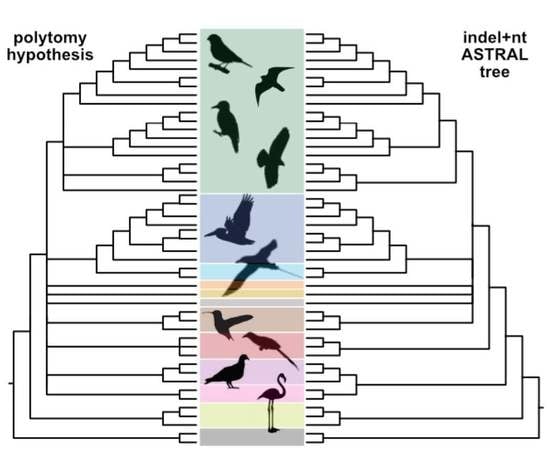
Figure 1.
Definitions of clade names used in this paper. The basal-most polytomy represents “the magnificent seven” and three “orphan orders” of Reddy et al. [18]. Other polytomies reflect differences in tree topologies recovered using various data types and analyses (reviewed by Braun et al. [1]).

Figure 2.
Evidence for extensive gene tree–species tree conflict at the base of Neoaves. (a) Total Evidence Nucleotide Tree (TENT) maximum likelihood (ML) tree of Jarvis et al. [15] with branch lengths in mutation units, drawn using Interactive Tree Of Life (iTOL) [23]. Branches are colored by Quartet Score (QS) computed using ASTRAL based on all 14,446 unbinned nt gene trees with branches that have bootstrap support (BS) ≤5% contracted. Low QS (red) in deep divergences among Neoaves are suggestive of high levels of ILS. The null hypothesis of a polytomy could not be rejected for four branches (dashed lines) at the p < 0.01 level (p-values shown in green on nodes where the null hypothesis is rejected) [19]; (b) ASTRAL-III tree run on all 14,446 unbinned nt gene trees with branches with BS ≤5% contracted, as reported by [24,25]. Branch lengths in coalescent units computed by ASTRAL are written under each branch. Branch colors are identical to (a). The null hypothesis of a polytomy could not be rejected for six branches (dashed lines) at the p < 0.01 level (p-values shown in green on nodes where the null hypothesis is rejected).

Figure 3.
Numbers of indels and estimates of their homoplasy are related to indel size. Indel frequency (blue; log scale) and the percentage of indels that are parsimony consistent (red) as a function of indel length (log scale). We defined indels as parsimony consistent if they have RI = 1.0 on a specific tree. We used the “Total Evidence Indel Tree” (TEIT; Figure S12 in Jarvis et al. [15]) as that estimate of the avian species tree because it reflects indel data (it is based on concatenated exon, intron, and UCE indels). The curve for the percentage of parsimony consistent indels resembles a step function. This likely reflects the fact that the accumulation of indels over evolutionary time involves multiple mechanisms. The case where 100% of the characters have RI = 1.0 (i.e., the situation for the largest indels above) is consistent with the absence of true homoplasy as well as complete lineage sorting.

Figure 4.
Frequency distribution of ensemble retention index (RI) calculated using individual gene trees by intron indel gene trees, UCE indel gene trees, intron nt gene trees, and UCE nt gene trees. Ensemble RI of individual loci should provide a more accurate measure of homoplasy than RI of species trees by minimizing the role of hemiplasy. Indel gene trees exhibit substantially higher RI than nt gene trees.

Figure 5.
Gene tree resolution for intron and UCE gene trees estimated from indel and nt data. (a) Boxplots show the number of binary nodes, normalized by the maximum possible number of binary nodes (e.g., 46 for gene trees with no missing data) for gene trees where nodes with BS up to a certain threshold (x-axis) are contracted. With no contraction, this value is 1.0 and with increased filtering, it quickly drops; (b) The density of the gene tree BS averaged over all branches of each gene tree are shown. Overall, nt gene trees are better supported than indels and introns are better supported than UCEs.

Figure 6.
RF distances for intron gene trees. Density of normalized RF distances between indel and nt gene trees of the same locus (red) are compared to distances between randomly sampled indel gene trees and randomly sampled nt gene trees. Randomly sampled nt gene trees are slightly more congruent with one another than indel and nt gene trees of the same locus. Indel and nt gene trees of the same locus are substantially more congruent with one another than randomly sampled indel gene trees. Similar patterns are observed for UCE gene trees (Figure S9).

Figure 7.
Comparison of quartet frequencies for combined intron+UCE nt+indel gene trees. (a) ASTRAL tree using all 12,388 gene trees from combined intron+UCE nt+indel datasets with branches with up to 5% BS contracted. Branch labels are local posterior probabilities (localPP) <1.0. In computing localPP, two gene trees from the same locus are counted as one to avoid double counting the same locus. Branches where the polytomy could not be rejected using the polytomy test in ASTRAL at the 0.05 significance level are marked with a #; (b) Right panel: the same tree as above with collapsed branches, and remaining branches labeled 1 to 65; Left panel: quartet frequency of the main resolution (red bar) and the two alternative resolutions around that branch (blue bars) for all labeled internal branches. Labels on the x-axis indicate the quartet topology. For example, for box “37”, the second set of bars puts “36” and “59” together, meaning that the position of pelican and loon are swapped; the third bar puts “58” and “59” together, meaning that loon and pelican are put together. Quartet frequencies computed from combined nt gene trees (i.e., UCEs+introns) are shown in lighter tones and quartet frequencies based on combined indel gene trees are shown in darker tones. The horizontal dashed lines show the ⅓ threshold, which corresponds to either a true hard polytomy or random resolutions in gene trees. Nodes with high support (top) and low support (bottom) show two different scales. Note that many of the basal branches have quartet frequencies that are very close to ⅓.

Figure 8.
ASTRAL trees using intron (a,b) and UCE (c,d) loci with gene trees computed using nt (a,c) or indels (b,d) and branches with up to 5% BS contracted. Branch labels show localPP and those without a designation have a localPP of 1.0. Shades of grade correspond to the support value.
Figure 8.
ASTRAL trees using intron (a,b) and UCE (c,d) loci with gene trees computed using nt (a,c) or indels (b,d) and branches with up to 5% BS contracted. Branch labels show localPP and those without a designation have a localPP of 1.0. Shades of grade correspond to the support value.

Figure 9.
(a) For each focal relationship (i.e., those with some conflict), we show whether they are recovered or rejected in various trees with high or low support, defined by a threshold of 95% support. Three relevant trees from the Jarvis dataset and two MP indel trees are also included. Note that support values are localPP for ASTRAL trees and BS support for concatenation trees, including those from Jarvis et al. [15]. See Figure 1 for clade names. Figure created using DiscoVista. (b) The number of different branches between all pairs of ASTRAL species trees.

Figure 10.
QS of the ASTRAL tree computed from intron and UCE, indel and nt gene trees at levels of gene tree contraction from 0–33%. UCE indels yield uniformly lower QS than intron indels and nt data and removing low support branches increases the QS of the ASTRAL tree.
Figure 10.
QS of the ASTRAL tree computed from intron and UCE, indel and nt gene trees at levels of gene tree contraction from 0–33%. UCE indels yield uniformly lower QS than intron indels and nt data and removing low support branches increases the QS of the ASTRAL tree.

Figure 11.
ASTRAL trees using combined dataset gene trees with branches with up to 5% BS contracted. (a) Intron-combined = intron nt+indel gene trees; (b) UCE-combined = UCE nt+indel gene trees; (c) nt-combined = intron+UCE nt gene trees; and (d) indel-combined = intron+UCE indel gene trees. Branch labels are localPP <1.0. Note, in computing branch support of intron-combined and UCE-combined trees, every two gene trees of the same locus are counted as 1 to avoid double counting.

Figure 12.
Collapsed polytomy trees estimated by the hard polytomy test of combined intron+UCE nt+indel implemented in ASTRAL [19] (right) compared to the polytomous tree hypothesized by Suh [17] (left). This study reduces the scale of the basal neoavian hard polytomy from a radiation of nine lineages (or even ten lineages) to a radiation of six major lineages, i.e., core landbirds (Telluraves), pan-waterbirds (Aequornithia+Phaethontimorphae), Charadriiformes, Gruiformes, Hoatzin, and Caprimulgiformes (including swift+hummingbird).


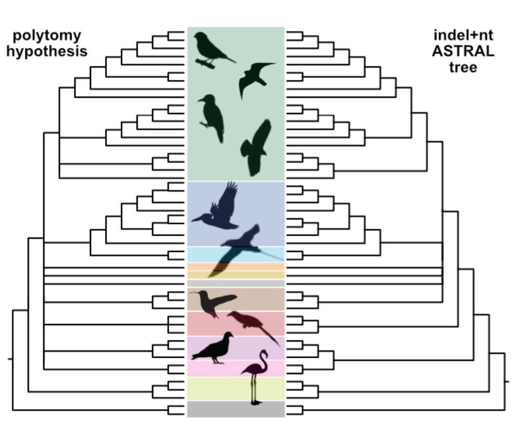
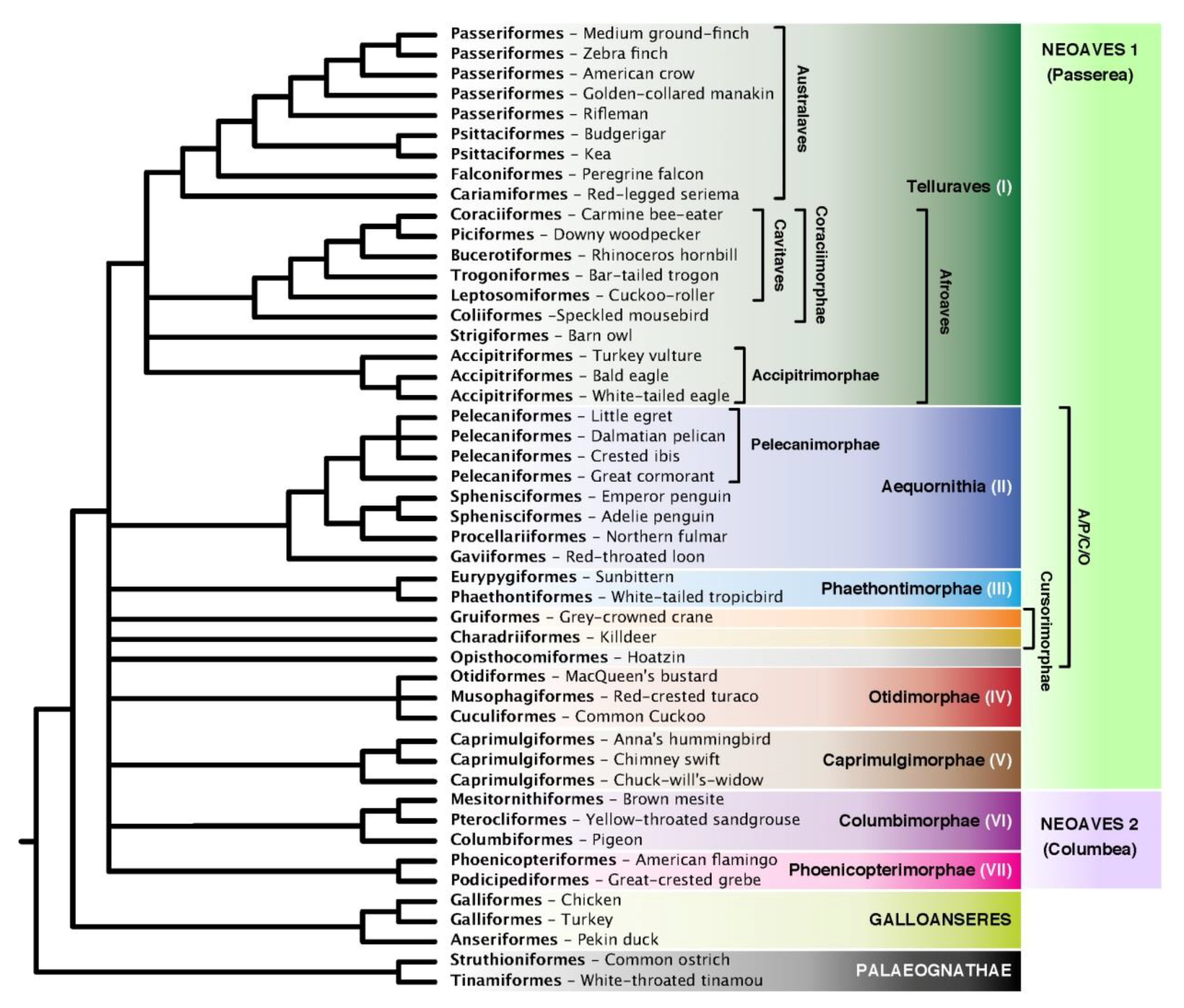
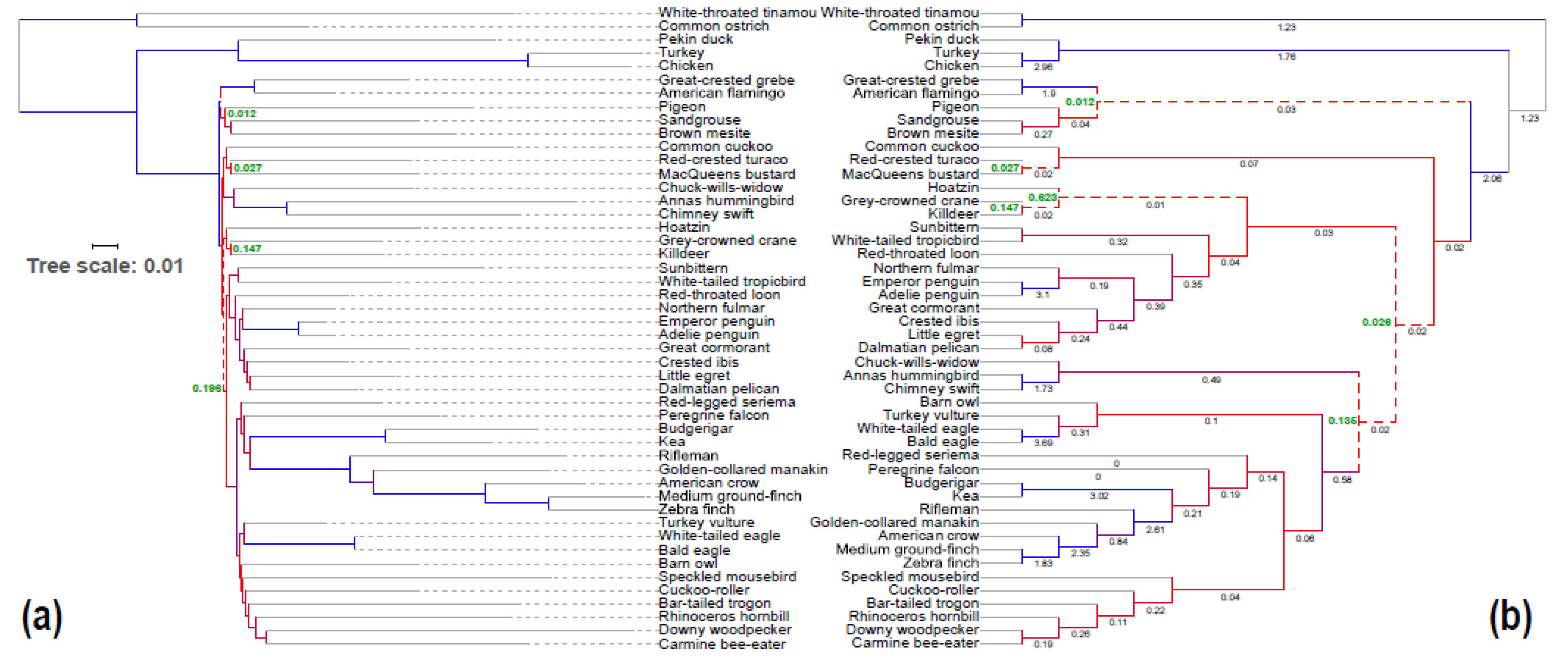
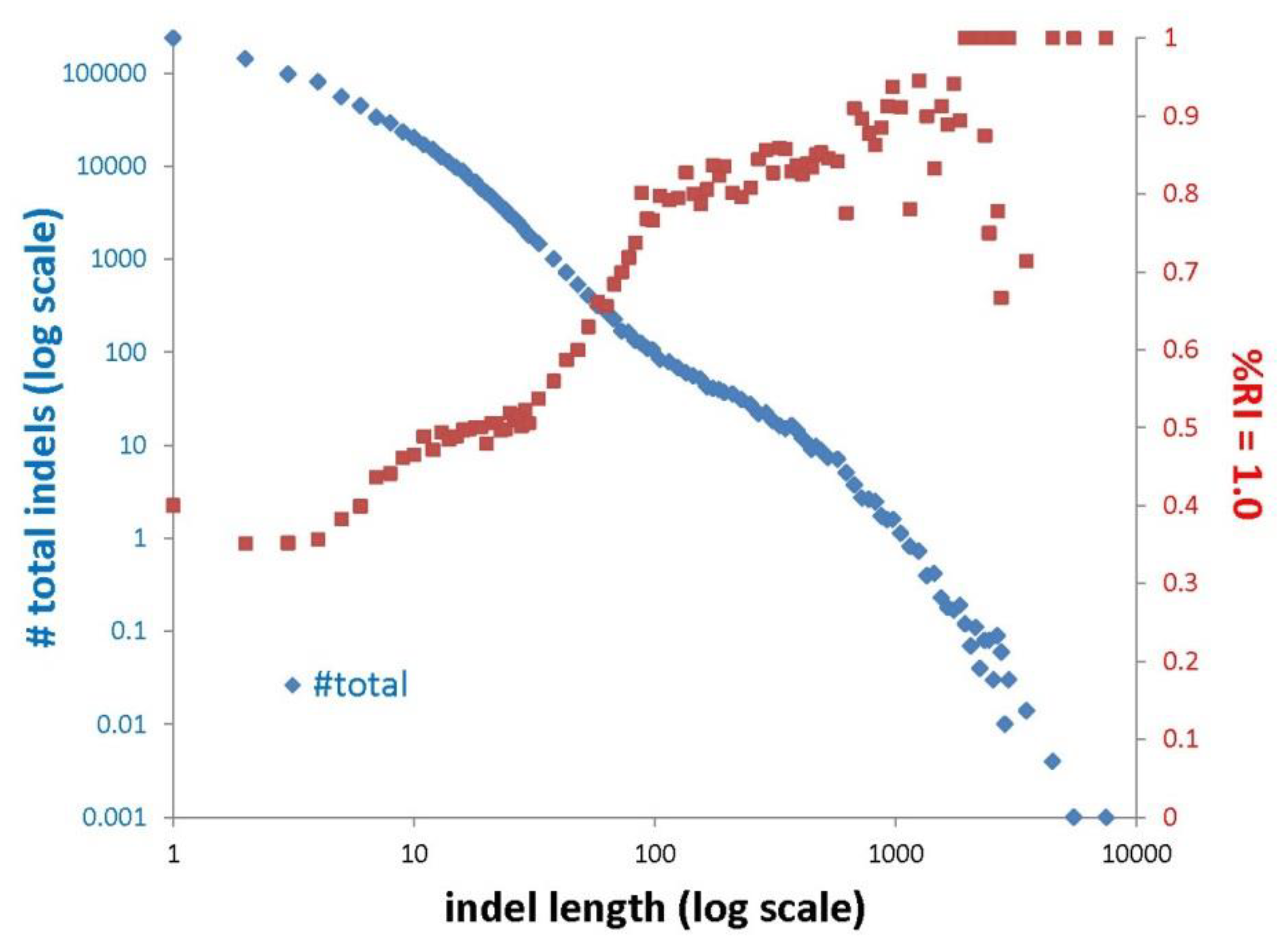
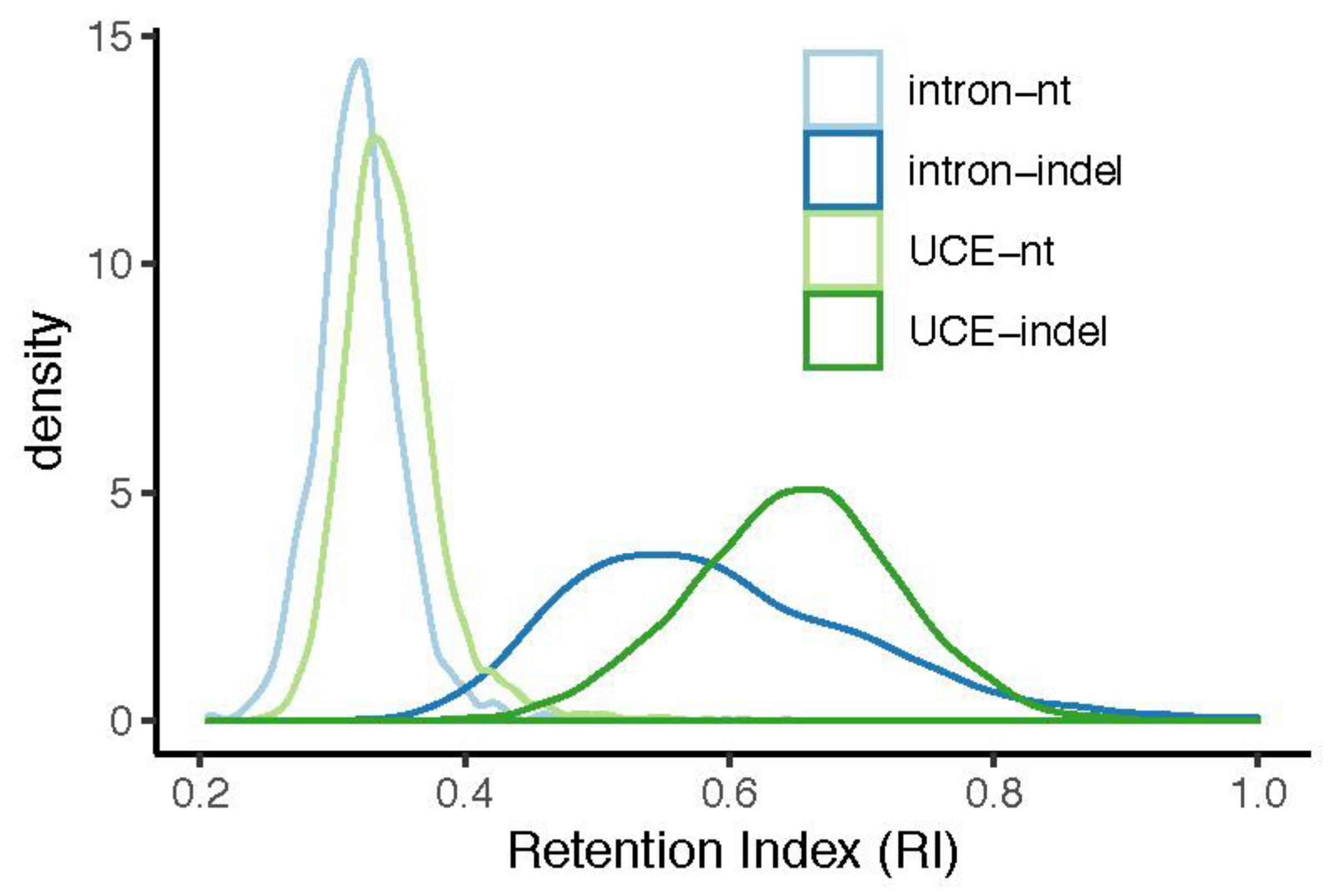
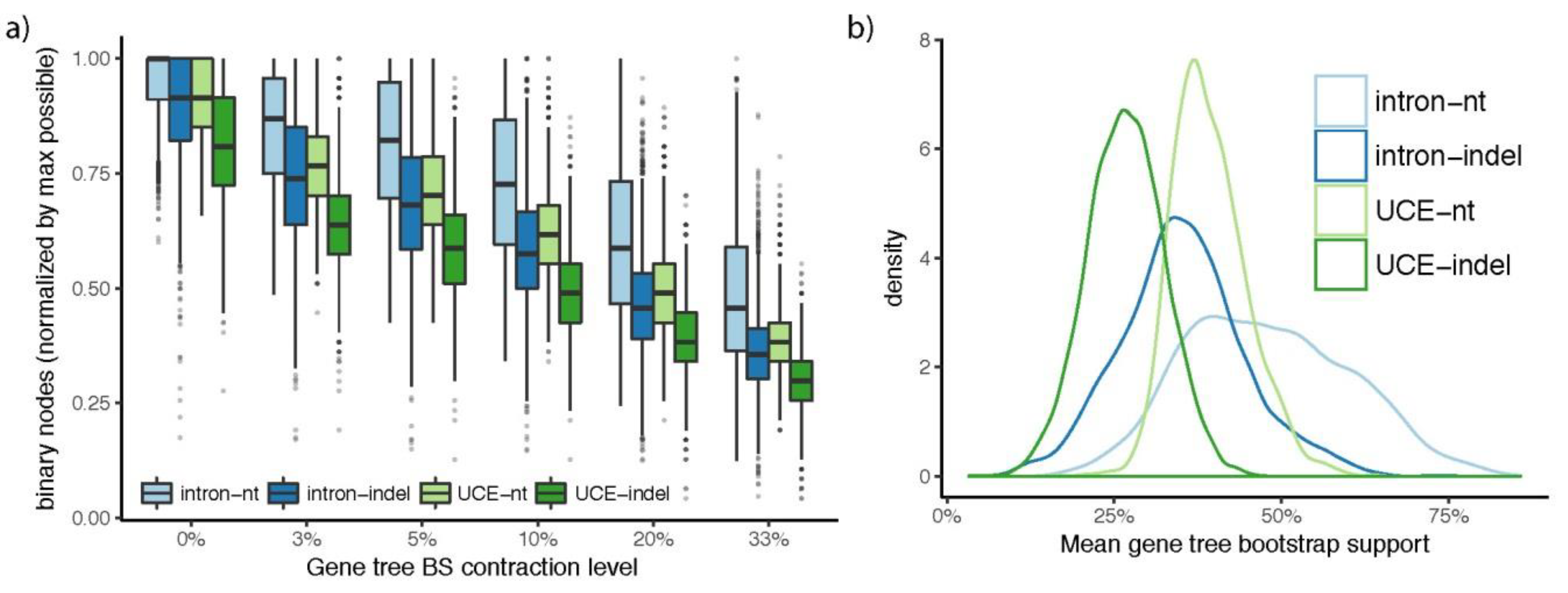
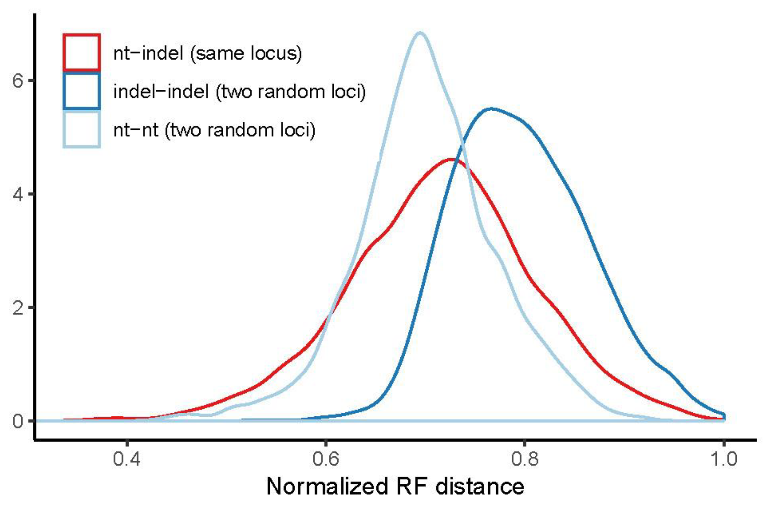
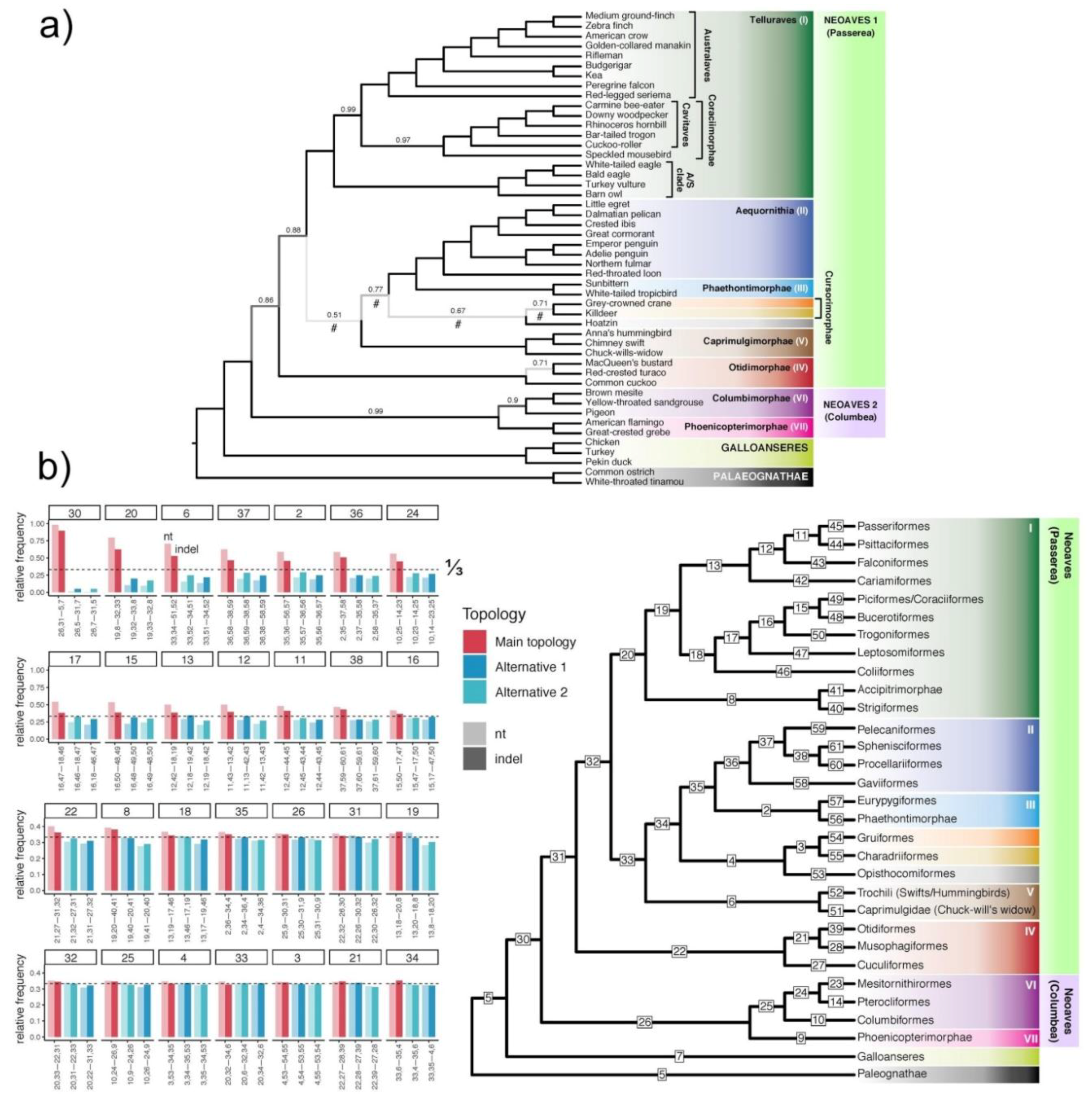
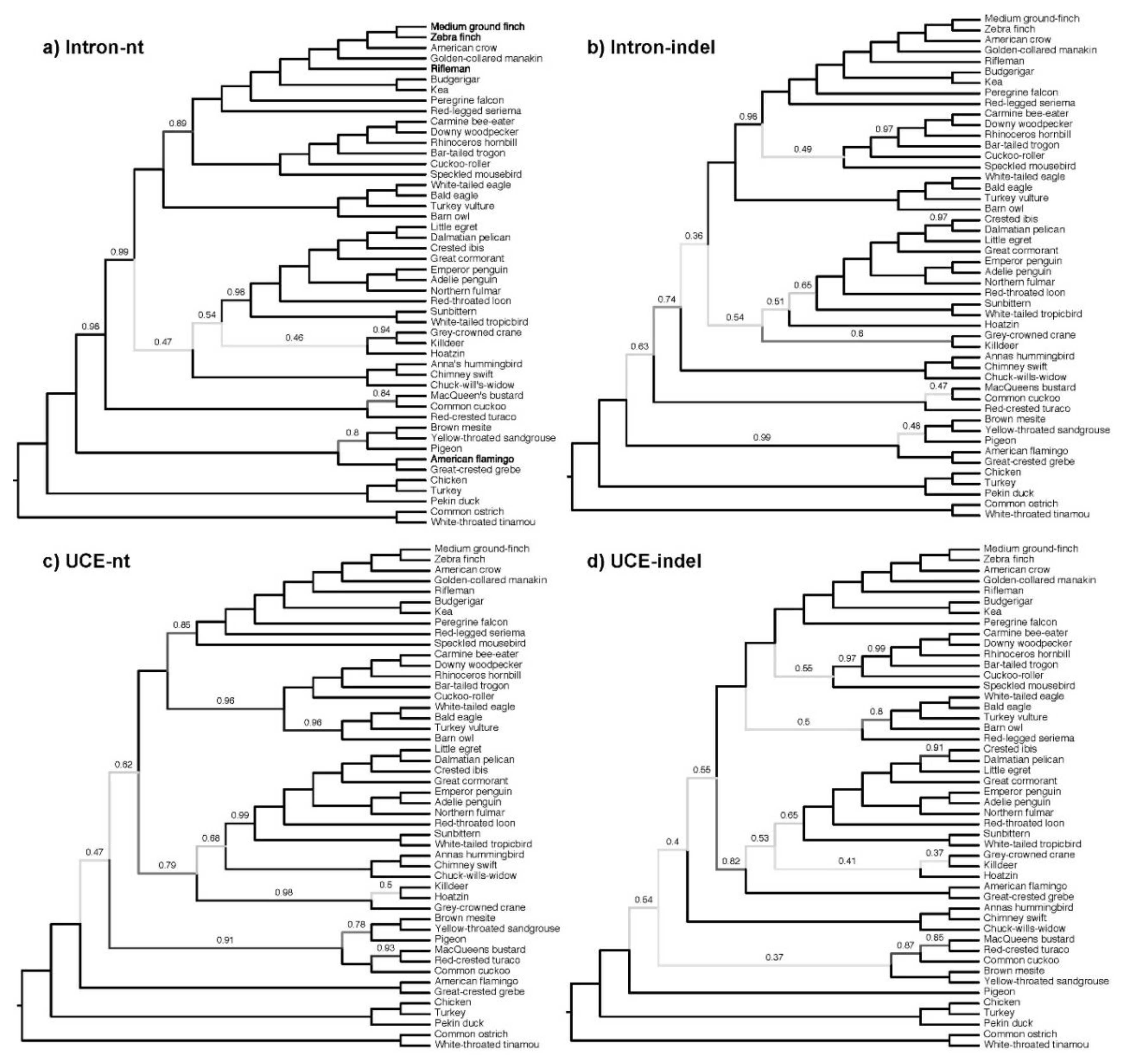
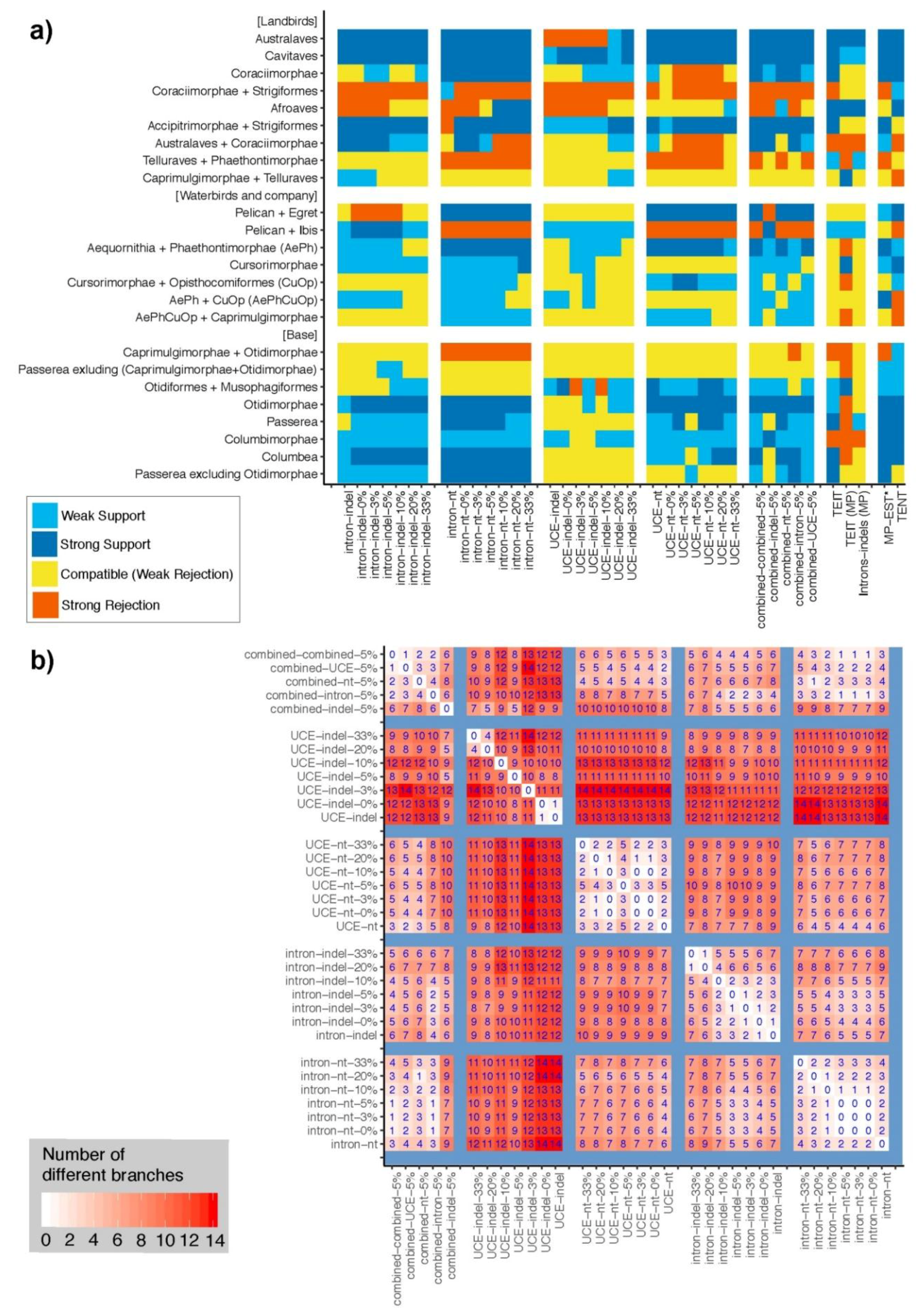
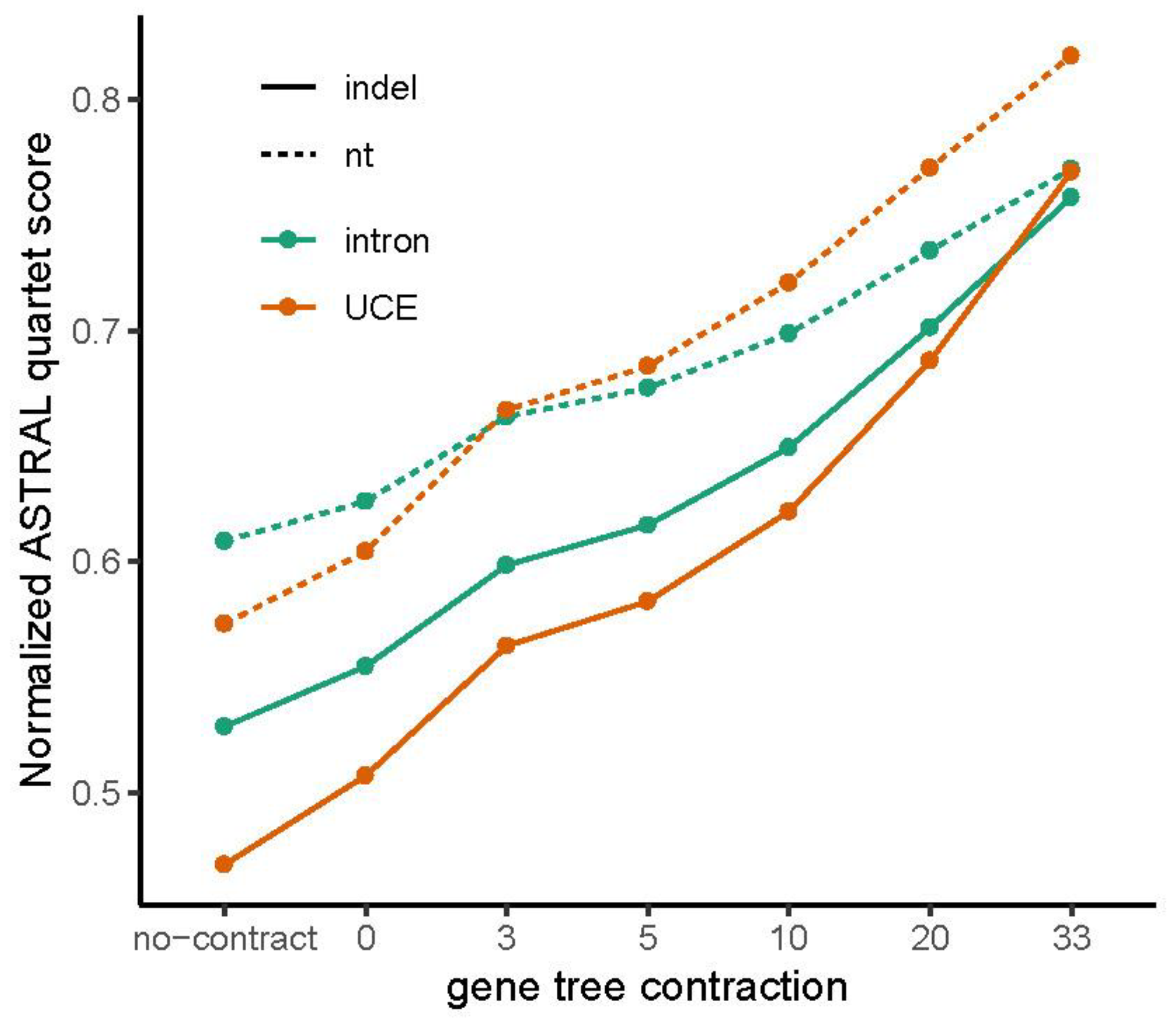
Table 1.
Indel and nt information content.
| Introns | Ultraconserved Elements (UCEs) | All Data | |
|---|---|---|---|
| Number (#) of loci | 2515 | 3679 | 6194 |
| Total # of nts | 19,258,212 | 9,229,346 | 28,487,558 |
| Total # of indels | 3,918,322 | 1,242,014 | 5,160,336 |
| # Parsimony Informative nts | 10,855,614 | 3,908,476 | 14,764,090 |
| # Parsimony Informative indels | 942,169 | 315,393 | 1,257,562 |
| % Parsimony Informative nts | 56.37 | 42.35 | 51.83 |
| % Parsimony Informative indels | 24.05 | 25.39 | 24.37 |
| Indels per locus: | |||
| Minimum | 6 | 10 | 6 |
| Lower quartile | 431.5 | 266 | 284 |
| Upper quartile | 2065 | 406.5 | 704 |
| Median | 1014 | 333 | 389 |
| Mean | 1,557.98 | 337.6 | 833.12 |
Table 2.
Intron indel number, information content, and parsimony consistency by size class.
| All | 1bp | 2–9bp | 10–49bp | 50–99bp | 100+bp | |
|---|---|---|---|---|---|---|
| # indels | 3,918,322 | 1,023,680 | 1,924,526 | 828,741 | 65,651 | 75,724 |
| # informative indels | 942,169 | 239,295 | 510,023 | 168,906 | 10,515 | 13,430 |
| % informative indels | 24.05 | 23.38 | 26.50 | 20.38 | 16.02 | 17.74 |
| Ensemble RI indels 1 | 0.52 | 0.54 | 0.49 | 0.56 | 0.73 | 0.86 |
| Ensemble RI nts 1 | 0.31 |
1 ensemble RI calculated as concatenated data on the Jarvis et al. ML TENT [15], not by locus.
Table 3.
Robinson–Foulds (RF) distances.
| Quartiles | indel–nt Same Locus | indel–indel Different Loci | nt–nt Different Loci |
|---|---|---|---|
| 1st quartile | 0.658 | 0.744 | 0.659 |
| median | 0.721 | 0.791 | 0.698 |
| 3rd quartile | 0.775 | 0.842 | 0.743 |
Table 4.
Number of incompatible branches between intron indel vs. nt gene trees.
| Tree Resolution | Same Locus Mean (SD) n = 2515 | Different Loci Mean (SD) n = 6322710 |
|---|---|---|
| Fully resolved | 30.06 (3.88) | 30.84 (2.90) |
| <34% contracted | 3.530 (2.61) | 4.138 (2.96) |
| <76% contracted | 0.192 (0.50) | 0.343 (0.72) |
© 2019 by the authors. Licensee MDPI, Basel, Switzerland. This article is an open access article distributed under the terms and conditions of the Creative Commons Attribution (CC BY) license (http://creativecommons.org/licenses/by/4.0/).
Share and Cite
MDPI and ACS Style
Houde, P.; Braun, E.L.; Narula, N.; Minjares, U.; Mirarab, S. Phylogenetic Signal of Indels and the Neoavian Radiation. Diversity 2019, 11, 108. https://doi.org/10.3390/d11070108
AMA Style
Houde P, Braun EL, Narula N, Minjares U, Mirarab S. Phylogenetic Signal of Indels and the Neoavian Radiation. Diversity. 2019; 11(7):108. https://doi.org/10.3390/d11070108
Chicago/Turabian StyleHoude, Peter, Edward L. Braun, Nitish Narula, Uriel Minjares, and Siavash Mirarab. 2019. "Phylogenetic Signal of Indels and the Neoavian Radiation" Diversity 11, no. 7: 108. https://doi.org/10.3390/d11070108
Note that from the first issue of 2016, this journal uses article numbers instead of page numbers. See further details here.