Article

Simulation of Polymer Crystallization under Isothermal and Temperature Gradient Conditions Using Particle Level Set Method

1
Department of Applied Mathematics, Northwestern Polytechnical University, Xi’an 710129, China
2
Department of Computational Mathematics, Henan University of Science and Technology, Luoyang 471003, China
*
Author to whom correspondence should be addressed.
Crystals 2016, 6(8), 90; https://doi.org/10.3390/cryst6080090
Submission received: 28 June 2016 / Revised: 27 July 2016 / Accepted: 1 August 2016 / Published: 8 August 2016
(This article belongs to the Special Issue Advances in Computer Simulation Studies on Crystal Growth)

Abstract

:
Morphological models for polymer crystallization under isothermal and temperature gradient conditions with a particle level set method are proposed. In these models, the particle level set method is used to improve the accuracy in studying crystal interaction. The predicted development of crystallinity during crystallization under quiescent isothermal condition by our model is reanalyzed with the Avrami model, and good agreement between the predicted and theoretical values is observed. In the temperature gradient, the computer simulation results with our model are consistent with the experiment results in the literature.

Graphical Abstract

1. Introduction

The final properties of a product produced from semi-crystalline polymer are to a great extent determined by the final internal microstructure [1,2]. This final internal microstructure, in turn, is determined by the crystallization/processing conditions. Therefore, it is very important to accurately model the solidification process and predict the final microstructure formed under different processing conditions.
To date, a number of investigators are interested in predicting the morphological development of polymer crystallization and many research studies have been carried out on this topic [2,3,4,5,6,7,8,9,10,11,12]. In order to obtain the internal microstructure of polymer products, different approaches have been proposed for morphological modeling of polymer crystallization by researchers [7,8,9,10,11,12]. Charbon and Swaminarayan [7,8] presented front-tracking methods to predict the evolution of microstructures during spherulitic crystallization under realistic crystallization conditions. Raabe and Godara [9] studied the topology of spherulite growth during crystallization of isotactic polypropylene (iPP) by using a cellular automata method. Xu and Bellehumeur [10,11] proposed a modified phase-field method to capture the spatiotemporal morphology development with the crystallization behavior of ethylene copolymers in the rotational-molding process. Ruan et al. [12] investigated the evolution of morphology of crystallization in the short fiber reinforced system using a pixel coloring method.
We presented a level set method for simulating the solidification structure of polymer crystallization during cooling stage in [13] to reduce the computation complexity in studying crystal interaction. In that method, each crystal can be distinguished from others by its assigned color, the problem of evolving multiple crystal interfaces is reduced to tracking one level set variable (signed distance function) and determining the color of a newly solidification node point. That method is easy to be implemented and it is also applicable for any system that displays nucleation and growth. However, just like other Eulerian methods, level set methods have the main drawback that they are not conservative [14,15,16] (see Figure 1a). To fix this problem, several attempts to improve mass conservation of level set methods have been done, such as the improved level set methods [16,17,18] and the particle level set methods [14,19]. In the particle level set method, particles that are distributed within both an interior and exterior band of the interface are used to preserve volume so as to maintain the interface. Literature [14] indicates the particle level set method compares favorably with volume of fluid methods in the conservation of mass and purely Lagrangian schemes for interface resolution.
In this paper, we aim to develop a more accurate interface tracking method for studying morphology of polymer crystallization, and further apply the proposed method to morphological models of iPP crystallization under isothermal and temperature gradient conditions. To achieve our goal, firstly, based on the method described earlier [13], we use a particle level set method instead of the level set method to correct any volume loss that resulted from advecting the level set. Secondly, because there already exist many particles in the particle level set method and the accuracy of Lagrangian advection, we use some of these particles to help to color the node points instead of using the semi-Lagrangian method that was used in [13]. Finally, for different temperature conditions, we use different method to deal with the problems in determining morphology of polymer crystallization.
The outline of this paper is as follows: Section 2 presents the particle level set method for polycrystals growth. In Section 3, the morphological modeling using the particle level set method for polymer crystallization under isothermal conditions is introduced. In Section 4, the extended algorithm for polymer crystallization in uniaxial linear temperature field is established. Section 5 gives the numerical results and discussions. Finally the conclusions are drawn in Section 6.

2. Particle Level Set for Polycrystals Growth

2.1. Level Set Method

The level set method was originally designed by Osher and Sethian [21,22] in 1988, and then it has been manipulated in moving interfaces of fluid mechanics, combustion, computer animation, image processing and some other interfaces of evolution problems. According to this method, the interface whose motion is recast as a time-dependent Eulerian initial value partial differential equation is denoted implicitly by the zero set of a continuous function.
A level set function φ ( x , t ) is defined as:
φ ( x , t ) = { + d ( x , t ) x Ω i n t e r i o r ( the solid regions ) 0 x Ω = Γ ( t ) ( the melt-solid interfce ) d ( x , t ) x Ω e x t e r i o r ( the melt regions )
where d ( x , t ) is set as the smallest distance between a given point in the domain Ω and the interface Γ ( t ) :
d ( x , t ) = min x Γ Γ x Ω ( | x x Γ | )
Additionally, the level set function has the following feature:
| φ | = 1
The instantaneous interface associates with the contour φ ( x , t ) = 0 , i.e.,
Γ ( t ) = ( x Ω : φ ( x , t ) = 0 )
The normal unit vector on the interface is expressed as:
n = φ | φ | | φ = 0
The equation for the evolution of φ corresponding to the motion of the interface is given by:
φ t + u φ = 0
where u represents velocity. With an evolution of the interface, the re-initialization is often necessarily due to a generally deviation of φ from its initialized value which represents signed distance. We apply the re-initialization until φ reach steady-state, i.e., the following equation is iterated:
φ t = φ 0 φ 0 2 + ε 2 ( 1 | φ | )
where φ 0 is the initial level set value to be re-initialized. When φ reaches steady-state, it satisfies the condition | φ | = 1 , i.e., φ is a signed distance. It is imperative for the formulation to remain well-posed as φ 0 if the parameter ε in Equation (7) is assigned some small value.

2.2. Particle Level Set Method

The main problem that the level set method suffers from is numerical dissipation. The particle level set method merges the best aspects of Eulerian front-capturing schemes and Lagrangian front-tracking methods for improved mass conservation. In the particle level set method, two sets of massless particles, positive and negative particles, which are placed within a band across the interface, are used to correct the level set function.
The particle correction procedures in the particle level set method are summarized as follows:
(i)
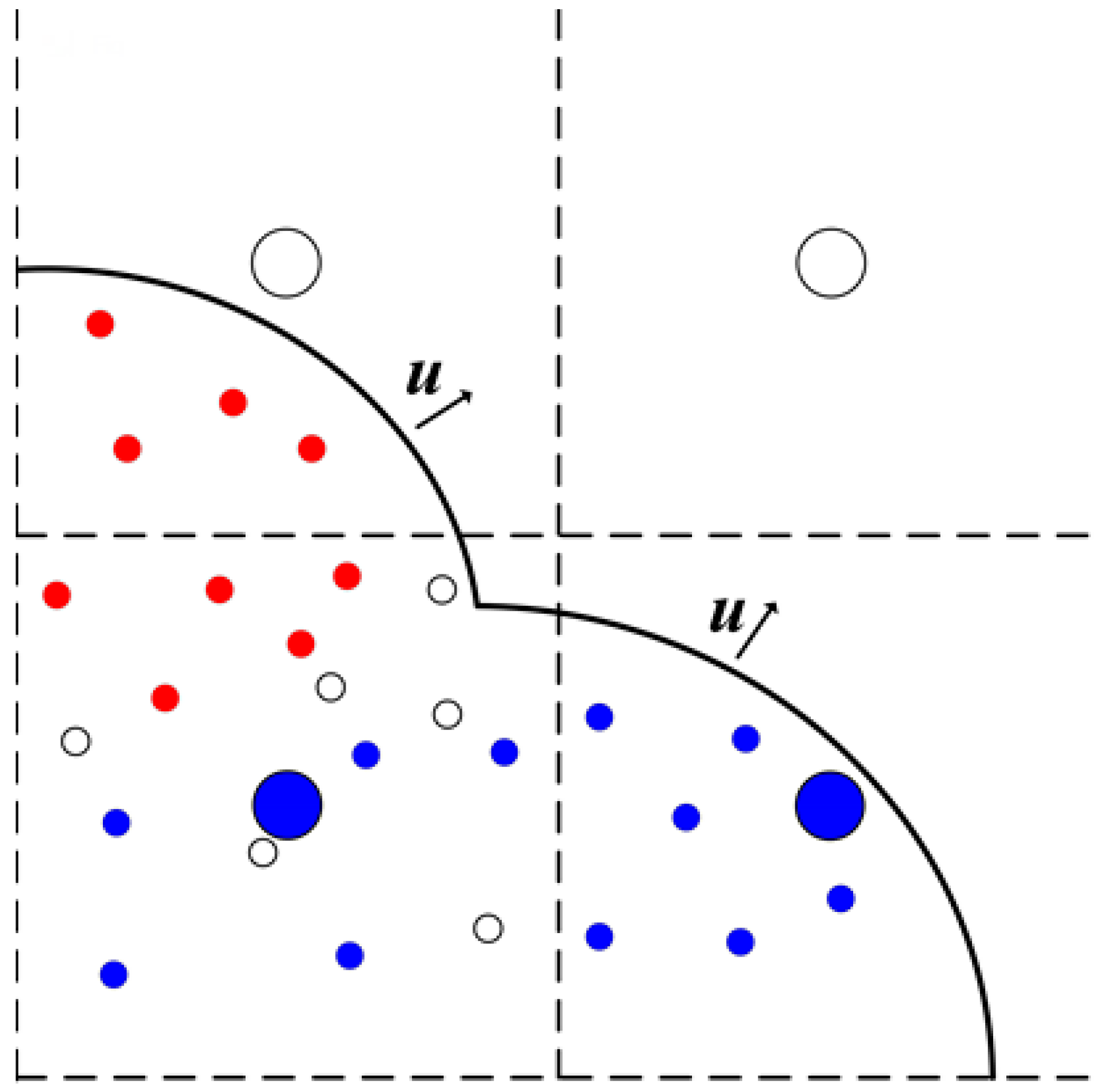
Particle initialization. When the initial surface is defined, the particles need to be placed within three cells of the interface. Each particle stores its position and radius, which is used to perform error correction on the level set function. The radius is set so that the boundary is just touching the interface:
r p = { r max i f s p φ ( x p ) > r max s p φ ( x p ) i f r min s p φ ( x p ) r max r min i f s p φ ( x p ) < r min
where r min = 0.1 min ( Δ x , Δ y ) , r max = 0.5 min ( Δ x , Δ y ) , and s p is the sign of the particle, set to +1 if φ ( x p ) > 0 and −1 if φ ( x p ) < 0. In [14], they recommend that 16 particles be placed in each cell in 2D.
(ii)
Particle update: The positions of the particles are updated using a second order Runga Kutta (RK2) time integration:
x p ( t + 1 ) = x p ( t ) + d t u t ( x p ( t ) )
x p * ( t + 1 ) = x p ( t + 1 ) + d t u t ( x p ( t + 1 ) )
x p ( t + 1 ) = x p * ( t + 1 ) + x p ( t ) 2
Error correction: Whenever a particle escapes the interface by more than its radius, it will be used to perform error correction on the interface. To enable error correction, a local level set value for each corner of the escaped particle is defined as follows:
φ p ( x ) = s p ( r p | x x p | )
Error correction is performed using the positive particles to create a temporary grid φ + and the negative particles to a temporary grid φ . For all of the escaped positive particles, the φ p values on cell corners containing the escaped particles are calculated by Equation (12), the value for each corner is then set to
φ + = max ( φ p , φ + )
Similarly, for all the escaped negative particles, the value for each corner is set to
φ = min ( φ p , φ )
Then, for each grid node, the minimum absolute value is chosen as the final correction for φ
φ = { φ + i f | φ + | | φ | φ i f | φ + | > | φ |
(iii)
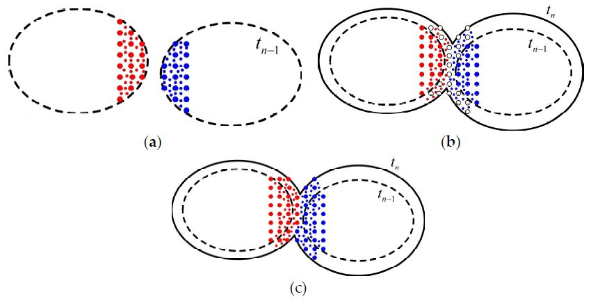
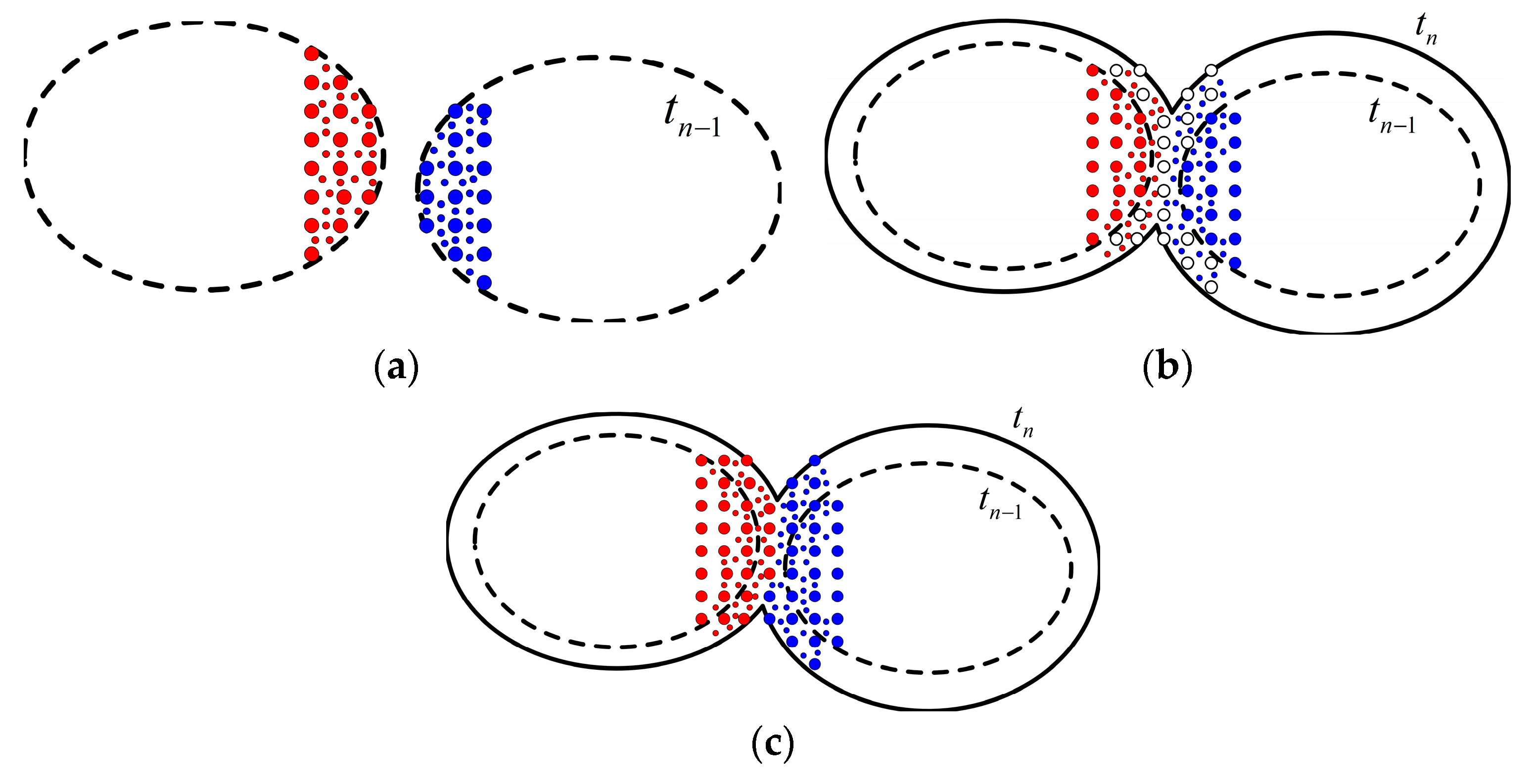
Particle reseeding: With the interface stretching and tearing, regions that lack a sufficient number of particles in the computational domain will form. Reseeding is carried out to delete the particles that are superfluous or far away from the interface and distribute a new set of particles to ensure that there is a uniform distribution of particles near the interface. It is important to note that if the simulation does not cause the particles to be unevenly distributed, there is no reason to reseed.
Further details of the particle level set method can be found in Reference [14]. The accuracy and efficiency of this method are shown in Figure 1b.

2.3. Particle Level Set Method for Polycrystals Growth

Typically, many crystals grow from individual seeds, and each of them will grow until it collides with other crystals and forms grain boundaries. Determining the contact boundaries is a difficult task. It is the reason why we employ a single signed distance to implicitly denote the interface of crystals and we also allot each crystal a “color” (respectively, a number) to distinguish different crystals. Because there already exists many particles in the particle level set method and the accuracy of Lagrangian advection, we detect the contact boundaries of crystals by these particles instead of the semi-Lagrangian method used in [13]. As demonstrated in Figure 2, the interfaces of two crystals are represented by the dotted lines, which are captured by the particle level set method at time t n 1 . The two crystals are differentiated by the colors of the nodes (the big circles), which lie in the two crystals respectively. To be used to color the nodes inside the two crystals at the next time step, the particles (the small circles) which are distributed inside the interfaces in the particle level set method are dyed in the same colors of the nodes near them (see Figure 2a). After one time step, the two crystals contact and we can capture their interfaces (denote with the solid lines) by the particle level set method, but the contacted boundary of the two crystals is not yet determined. Meanwhile, the colored particles move to the new positions, the undyed nodes inside the solid line and outside the dotted line are in the crystalline phase (Figure 2b). Here we need to determine which crystal these nodes belong to, i.e., what color should the undyed nodes be colored? Noting that the dyed particles that belong to the same crystal have the same color, we thus color each undyed node with the color of the nearest dyed particle, then the boundary of the two crystals is determined (Figure 2c). Additionally, we have to point out that firstly, the node coloring procedure can also applied to the growth of crystal before contact. Secondly, once particle reseeding is imperative, attention must be paid to color the particles that are placed into the cells where there exist different colored particles. The boundaries lie in these cells, so error boundaries can be resulted from any inappropriate coloring method. Maybe there is a better way to cope with this problem. In this study, we only use a simple technique: no coloring to these particles (Figure 3). This is the reason: on the one hand, it can ensure a sufficient number of particles in the computational domain; on the other hand, it would not lead to error results for the particles that are uncolored. More details of the particle level set method for polycrystals growth can be found in Section 3.

3. Morphological Model for Isothermal Crystallization of Polymer

Crystallization is a mechanism of phase change in semicrystalline polymeric materials. An isothermal crystallization process generally includes three steps, namely, nucleation, growth and impingement. Under the favorable thermodynamic condition, nuclei appear randomly in the polymer melt, and then the formed nuclei act as seeds for spherulites to grow with the same rate. Each spherulite grows until it impinges on adjacent spherulites and stops growing. Impingement takes place and continues until all possible material is transformed.

3.1. Nucleation

In semicrystalline polymers, the number of nuclei per unit volume or so-called nucleus density depends on the temperature and supercooling. Because the nucleation of semicrystalline polymers is typically heterogeneous, it is difficult to apply the theoretical models of the nucleation [4]. As a result, empirical approaches are adopted to solve this problem and nucleation laws are presented to represent the empirical relations between the nucleus density and the temperature. In the simulations, we use the following relation of the nucleation density [8,23]:
N = 1.458 { exp [ 111.265 0.2544 φ ( T + 273.15 ) ] } 2 / 3
where the unit of N is mm−2, and the unit of T is °C.

3.2. Growth and Impingement

Growth rate is an important factor that affects the development of morphology. Generally, for each polymer, the rate of crystal growth is a function of the crystallization temperature and can be considered a constant when the crystallization is considered under an isothermal condition. For a spherulite, the radial growth rate G can be calculated by applying the Hoffman–Lauritzen theory [24]:
G = G 0 exp [ U R g ( T T ) ] exp [ K g T Δ T ]
where G 0 and K g are constants, U is the activation energy of motion, R g is the gas constant, T is a temperature typically 30 K below the glass transition, and Δ T = T m 0 T is the degree of undercooling. It should be noted that, in the level set method, the velocity µ should be defined on the whole domain or on a narrow band near the interface. Therefore, we should extend the interface velocity away from the interface (solid/liquid boundary). There are many techniques to construct the extension velocity, details of which can be found in [25,26].
During the crystallization process, various stages of spherulite growth occur. In the early stages, probably no spherulites impinge. As the spherulites continue to grow, more and more of them will impinge each other. It is impingement that makes the grain boundaries form and the growth of spherulites stop. In fact, the shapes of the grains can directly influence the final properties of the polymers. In this study, the particle level set method for polycrystals growth is used to simulate the growth and impingement of spherulites.

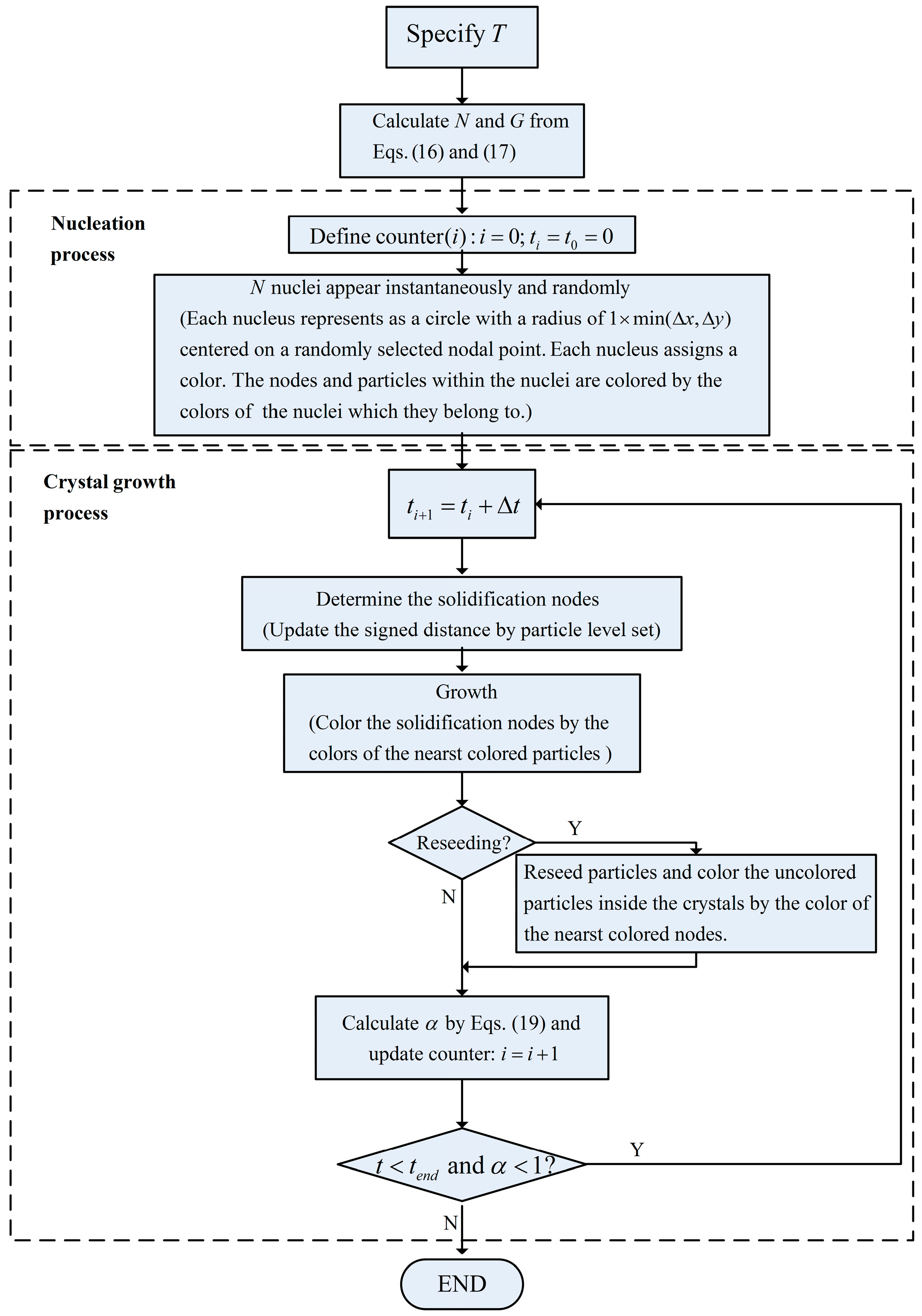
3.3. Algorithm for Polymer Crystallization under Isothermal Conditions

Under isothermal conditions, we use the stochastic method utilized in [13] to place the nucleation sites in the nucleation process. In this method, a node is chosen randomly in the computational domain when a new nucleus appears. Then a new color is allotted to this node and the signed distance field is updated with the following expression:
φ ( y ) = max ( φ 0 ( y ) , x y R 0 ) , y Ω
where x is the nucleation site, φ 0 is the signed distance before the potential nucleation site is nucleated at x , R 0 is the size of the initial crystal seed at location x , and y is the location of a node. It should be noted that, unlike in [13], in the nucleation process in this paper, the particles inside each crystal also need to be colored by the same color of the crystal. It is the colored particles that provide an effective way to distinguish different crystals after growth under different conditions.
In the crystal growth process, the particles inside the crystals are first used to correct the volume loss that resulted from advecting the level set in the particle level set method. Then they are utilized to color the uncolored nodes in the crystalline phase by their colors. If new particles need to be added to the computational zone, the way to color them is introduced in Section 2.3.
In our scheme, the relative crystallinity can be calculated by [13]:
α = n u m b e r o f n o d e s t h a t h a v e b e e n c o l o r e d t o t a l n u m b e r o f n o d e s
In addition, the mean of the maximum size of spherulites is defined as:
R ¯ max = ( A N π ) 1 / 2
where A is the volume of the spherulites which can be calculated with the number of notes occupied by the spherulites and the volume of a cell, and N is the number of the spherulites.
Figure 4 shows the algorithm for polymer crystallization under isothermal conditions using the particle level set method.

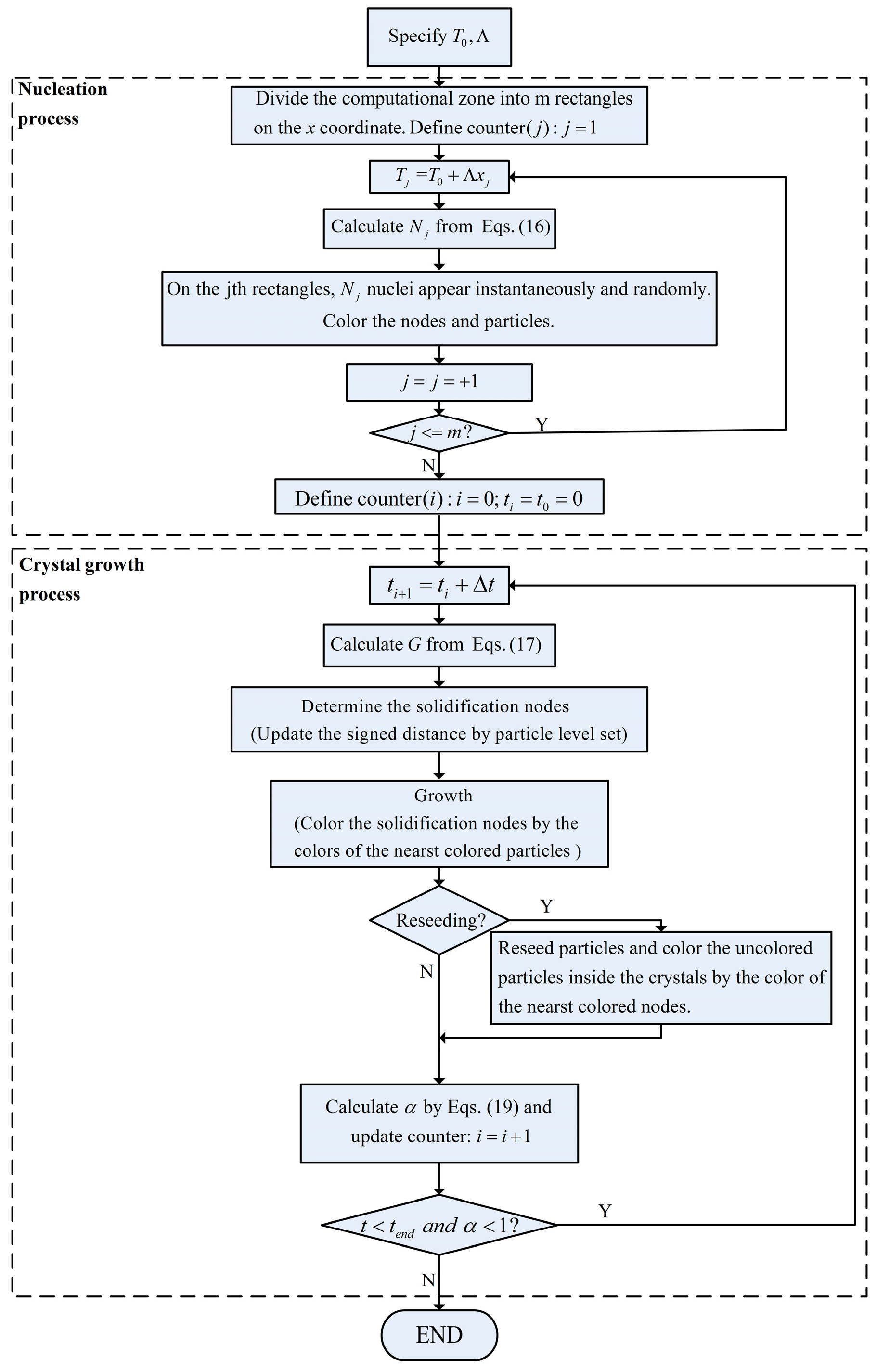
4. Morphological Model for Polymer Crystallization in a Temperature Gradient

In this paper, the polymer crystallization in a temperature gradient is modeled in a uniaxial linear temperature field: T = T 0 + Λ x . It is obvious when Λ = 0 , T = T 0 , the temperature is constant, i.e., it is isothermal. Thus, we need to extend the algorithm presented in Figure 4 to the uniaxial linear temperature field. To do this, on the one hand, we divide the computational zone into a series of small enough rectangles with respect to the x coordinate, so as to place the nucleation sites into the computational zone. In each small rectangle, the temperature is considered equal to that at the middle line of the vertical side on calculating the number of nuclei by Equation (16), and also the positions of spherulite nuclei are randomly chosen. On the other hand, G ( T ) needs to be recalculated on the x coordinate by G ( T 0 + Λ x ) each time step. With these preparations, the extended algorithm for polymer crystallization in the uniaxial linear temperature field using the particle level set method is shown as follows (Figure 5).

5. Results and Discussion

5.1. Problem Formulation

We consider the graphical simulation of the crystallization process on square samples. The maximum size of the samples is 600 µm × 600 µm. In order to ensure each unit cell is no more than the real space of 1 µm2 a regular mesh of 601 × 601 nodes is selected to solve this problem. It should be pointed out that the finer the unite cell the more accurate of the computational results. However, the finer the unit cell the more CPU time is needed. The material used in this simulation is an iPP and parameters used are listed in Table 1 [23].

5.2. Isothermal Case

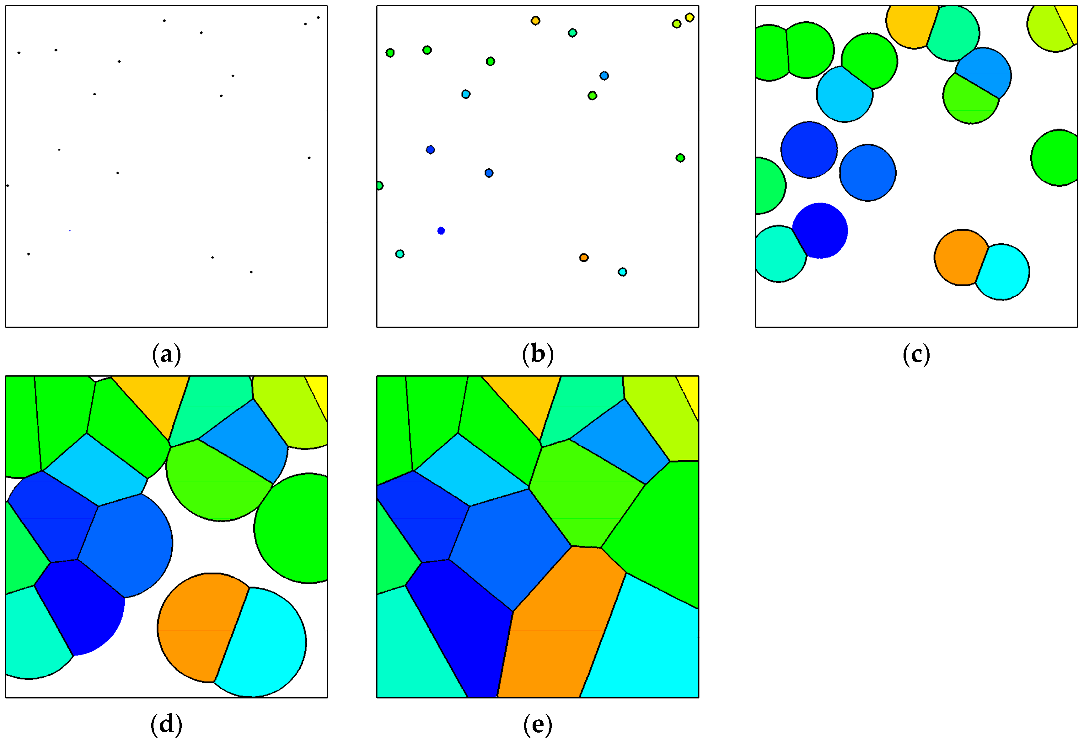
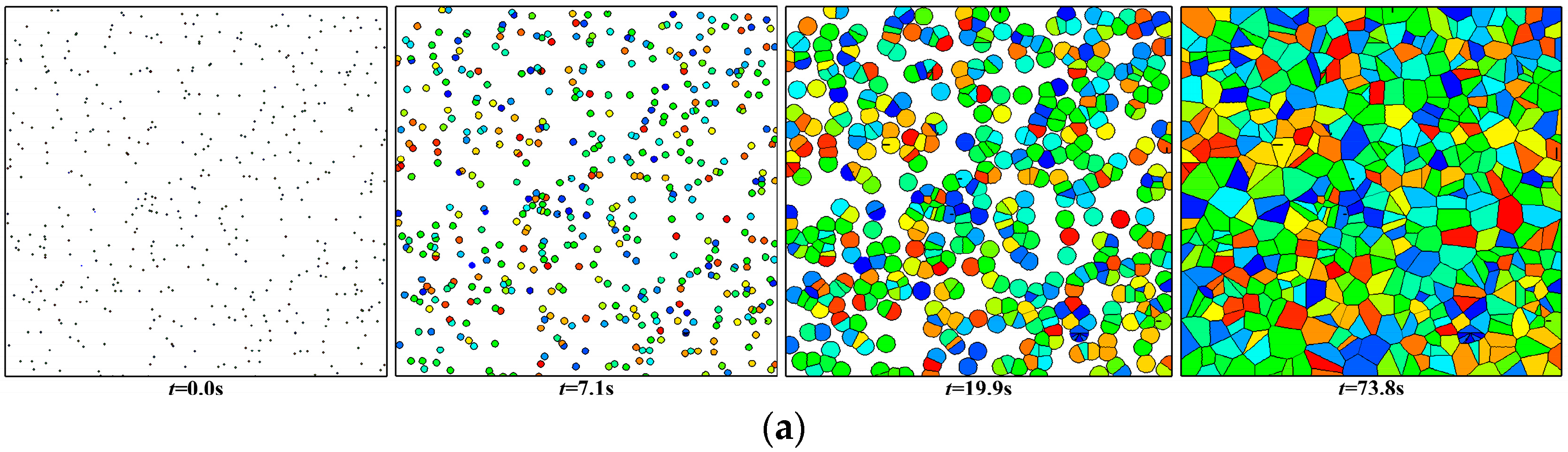
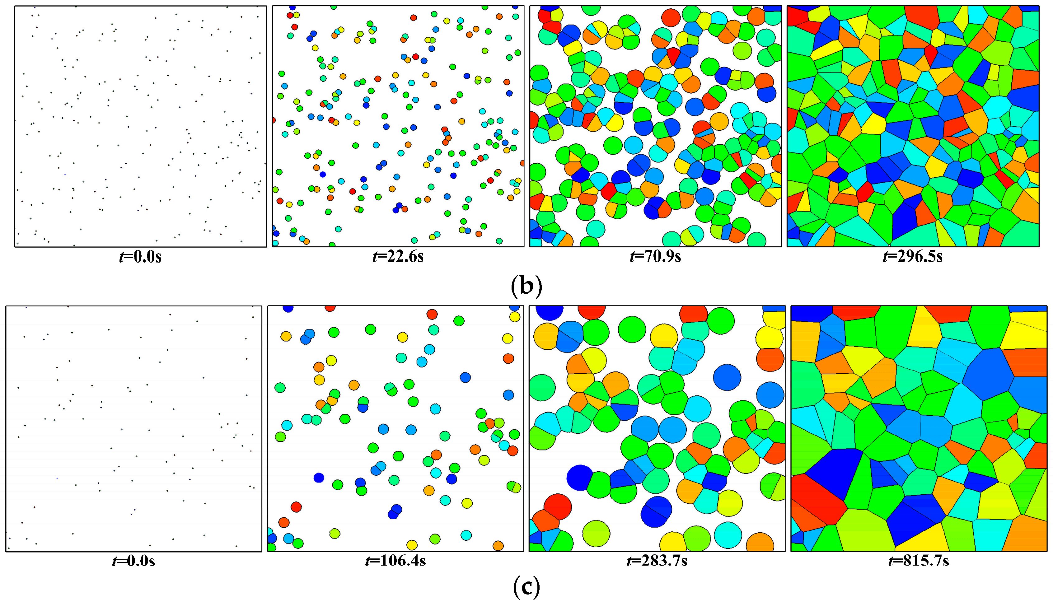
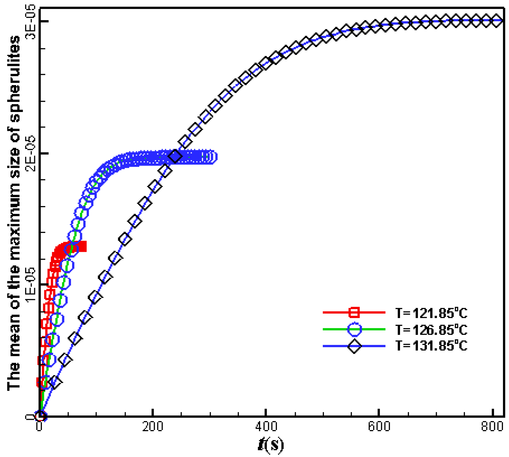
5.2.1. Morphological Development

Figure 6 shows the morphological development of iPP at T = 106.85 °C acquired from the algorithm for polymer crystallization under isothermal conditions by the particle level set method, the size of the square is 160 µm × 160 µm. As is illustrated in the Figure 6, in the process of evolutionary, the white region is polymer melt and the other colored region is crystals. Figure 6a illustrates iPP morphology at t = 0 s when heterogeneous nucleation takes place. Then each spherulite grows individually without impingement (Figure 6b) until t = 6.8 s, as time goes by, adjacent crystals touch and intercrystalline impingement boundaries arise (Figure 6c,d). Finally, we depict the final morphology (Figure 6e). We notice that the structures and characteristics of crystals obtained in this study are in accordance with the literature [27]. Figure 7 shows the evolution of crystal morphology with different temperatures and a square size of 500 µm × 500 µm. It is obvious that the lower the temperature the faster the crystallization time, the more the number of spherulites and the smaller size of the final grain. Figure 8 is plotted to demonstrate the mean of the maximum size of spherulites against time with different temperatures, and we observe that the mean of the maximum size of spherulites rises rapidly as time increases and reaches a plateau finally. Moreover, we perceive that the crystallization time becomes longer as the temperature rises. Apparently, we obtain many of the same conclusions analyzing Figure 7 and Figure 8.

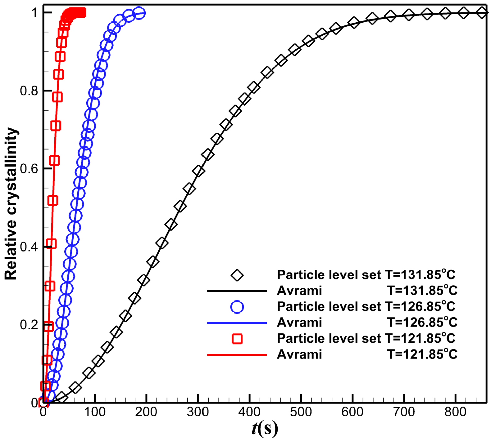
5.2.2. Overall Crystallization Kinetics

The most generally used approach for the description of the isothermal polymer crystallization kinetics is the Avrami model [28,29]. In the Avrami model, the relative crystallinity α ( t ) is usually written in the following form:
α ( t ) = 1 exp ( k a t n a )
where k a and n a are the isothermal crystallization rate constant and the Avrami index (crystal geometry information), respectively. In our study, heterogeneous nucleation and spherulitic morphology are assumed. Following [30], we take n a = 2 , k a = π N ( T ) [ G ( T ) ] 2 . Thus, Equation (21) can be rewritten as:
α ( t ) = 1 exp { π N ( T ) [ G ( T ) ] 2 t 2 }
Figure 9 displays the relative crystallinity evolution under different temperatures in isothermal condition. Symbols represent the predicted results, and lines represent the analytical solutions according to Avrami model. It is clear that the predicted results show good agreement with the theoretical values.

5.3. Temperature Gradient Case

In our simulations, the temperature gradient in the sample is parallel to the x axis, and the temperature, T, increases from the left to the right.

5.3.1. Effects of Temperature Gradient

In order to better illustrate the effects of temperature gradient, we assume that there is no other spherulite except the one(s) given in the computational domain in this section. The reasons for this are listed as follows. First, the fewer the number of spherulites in the computational domain, the more obvious the effect of the temperature gradient becomes. Second, different polymer material has different nucleation density at the same temperature. Therefore, even if we limit the numbers of nuclei, we can also obtain meaningful simulation results by selecting sizes of the samples appropriately.
Figure 10 shows the spherulite shapes predicted by the particle level set method for different temperature gradient. The sizes of these samples are 400 µm × 400 µm. In Figure 10a, the temperature gradient, Λ , equal to 50 °C·mm−1; and in Figure 10b, Λ = 100 °C·mm−1. As we can see in these two figures, the temperature gradient results in the spherulite shape anisotropy, which increases with time. Besides, in spite of the centers of the two spherulites are all locate at 130 °C, the shapes of them are quite different at the same moment (see Figure 10c). The main reason for this is that different temperature gradient makes the temperature distributions different on both sides of the center, and different temperature leads to different growth rate (see Figure 11). Figure 12 shows the shapes of interspherulitic boundaries in different temperature gradients of samples with sample size: 200 µm × 200 µm. We can see that, the three spherulites nucleate at the same sites in the three samples and the temperatures on the left side of the samples are all 110 °C, while the shapes of interspherulitic boundaries are very different. It is clear when Λ = 0 °C·mm−1, the boundaries are straight lines, but as the temperature gradient is higher, the boundaries bend toward higher T, and the curvature of the boundaries also increases.

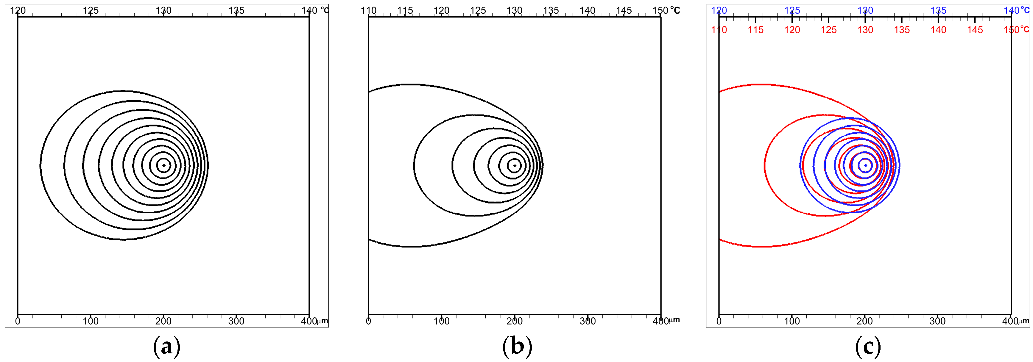
5.3.2. Morphological Development

In order to validate our model using the particle level set method for polymer crystallization in a temperature gradient, we simulate iPP film crystallization in the temperature gradient of 35 °C·mm−1. To compare our results to those in [23,31], all parameters utilized in the literature are also used in this simulation (see Table 1). The size of this sample is 600 µm × 600 µm. As we can see from Figure 13, the temperature gradient affects not only the nucleation density but also the spherulitic pattern. Figure 13a shows the spherulites only nucleate at the low-temperature side. Figure 13b,c demonstrates that the spherulites grow faster toward the low-temperature side and soon impinge on each other. The spherulites can still grow toward the high-temperature side, as shown in Figure 13d–f. We can also see that, in Figure 13f, the spherulites in the high-temperature side are elongated in shape, the collision boundaries of them are almost parallel to the temperature gradient, but the joint growth front of them is perpendicular to the temperature gradient. Figure 14 shows the computer-simulated positions of the crystallization front in the iPP film during crystallization in the uniaxial linear temperature field. The simulated results are in good agreement with the experiment and calculated results in the literature [23,31]. It indicates the correctness of our model.

6. Conclusions

We have presented an efficient particle level set method for polycrystals growth. In this method, the particles placed within an interior band of the interface in the particle level set method are used not only to correct any volume loss that resulted from advecting the level set and but also to determine the boundaries of crystals. With this method, an algorithm for polymer crystallization under quiescent isothermal condition has been developed. By the simulation model, for iPP, not only have we predicted the crystal morphological development and its distributions, but we have also obtained the relative crystalline and the mean of the maximum size of spherulites at different temperature T. The predicted development of crystallinity during crystallization has been reanalyzed with the Avrami model, and good agreement between the predicted and theoretical values has been observed.
We have also extended the algorithm from isothermal to temperature gradient conditions. In the uniaxial linear temperature field, we have presented a new method to place the nuclei in the computational zone. Numerical experiments have been used to analyze the effects of the temperature gradient. We also have simulated iPP film crystallization in the temperature gradient. The computer simulation results are consistent with the experiment results in the literature.
It should also be pointed out that the method used in this paper has two advantages compared with that in [13]: First, the particle level set method preserves volume better than the level set method. Thus, to the crystals with sharp edges, such as dendrites, more accurate crystallinity can be acquired. Second, as more particles are used to color the nodes, more precise boundaries of the crystals can be achieved. However, there are always two sides to everything, even if the particles utilized to color the nodes are also used in the original particle level set method, that more particles are used in this method increases the computational cost. In addition, the method cannot be used to determine the trajectory of the fibrils. However, this problem might be solved if we consider the trajectory of the particles, which are used in this method.
All in all, the morphological models for polymer crystallization under different conditions proposed in this study are valid. The calculated results with them give us another way to observe the microstructure of polymer products.

Acknowledgments

This work was financially supported by the National Basic Research Program of China (973 Program, contract Grant Number: 2012CB025903), the Major Research plan of the National Natural Science Foundation of China (Contract Number: 91434201), and the Natural Sciences Foundation of China (Contract Number: 11402078), which are gratefully acknowledged.

Author Contributions

Zhijun Liu and Jie Ouyang conceived the idea, developed the models and wrote the paper. Chunlei Ruan and Qingsheng Liu performed the computations and analyzed the results.

Conflicts of Interest

The authors declare no conflict of interest.

References

  1. Zhou, H.M. Computer Modeling for Injection Molding: Simulation, Optimization, and Control; John Wiley & Son: Hoboken, NJ, USA, 2012. [Google Scholar]
  2. Zheng, R.; Tanner, R.; Fan, X.J. Injection Molding: Integration of Theory and Modeling Methods; Springer: Berlin, Germany, 2011. [Google Scholar]
  3. Spina, R.; Spekowius, M.; Hopmann, C. Multiphysics simulation of thermoplastic polymer crystallization. Mater. Des. 2016, 95, 455–469. [Google Scholar] [CrossRef]
  4. Spina, R.; Spekowius, M.; Dahlmann, R.; Hopmann, C. Analysis of polymer crystallization and residual stresses in injection molded parts. Int. J. Precis. Eng. Manuf. 2014, 15, 89–96. [Google Scholar] [CrossRef]
  5. Roozemond, P.C.; van Erp, T.B.; Peters, G.W.M. Flow-induced crystallization of isotactic polypropylene: Modeling formation of multiple crystal phases and morphologies. Polymer 2016, 89, 69–80. [Google Scholar] [CrossRef]
  6. Xu, K.L.; Guo, B.H.; Reiter, R.; Xu, J. Simulation of secondary nucleation of polymer crystallization via a model of microscopic kinetics. Chin. Chem. Lett. 2015, 26, 1105–1108. [Google Scholar] [CrossRef]
  7. Swaminarayan, S.; Charbon, C. A multiscale model for polymer crystallization. I: Growth of individual spherulites. Polym. Eng. Sci. 1998, 38, 634–643. [Google Scholar] [CrossRef]
  8. Charbon, C.; Swaminarayan, S. A multiscale model for polymer crystallization. II: Solidification of a macroscopic part. Polym. Eng. Sci. 1998, 38, 644–656. [Google Scholar] [CrossRef]
  9. Raabe, D.; Godara, A. Mesoscale simulation of the kinetics and topology of spherulite growth during crystallization of isotactic polypropylene (iPP) by using a cellular automaton. Model. Simul. Mater. Sci. Eng. 2005, 13, 733–751. [Google Scholar] [CrossRef]
  10. Xu, H.; Bellehumeur, C.T. Modeling the morphology development of ethylene copolymers in rotational molding. J. Appl. Polym. Sci. 2006, 102, 5903–5917. [Google Scholar] [CrossRef]
  11. Xu, H.; Bellehumeur, C.T. Morphology development for single-site ethylene copolymers in rotational molding. J. Appl. Polym. Sci. 2008, 107, 236–245. [Google Scholar] [CrossRef]
  12. Ruan, C.; Ouyang, J.; Liu, S. Multi-scale modeling and simulation of crystallization during cooling in short fiber reinforced composites. Int. J. Heat Mass Transf. 2012, 55, 1911–1921. [Google Scholar] [CrossRef]
  13. Liu, Z.J.; Ouyang, J.; Zhou, W.; Wang, X.D. Numerical simulation of the polymer crystallization during cooling stage by using level set method. Comput. Mater. Sci. 2015, 97, 245–253. [Google Scholar] [CrossRef]
  14. Enright, D.; Fedkiw, R.; Ferziger, J.; Mitchell, I. A hybrid particle level set method for improved interface capturing. J. Comput. Phys. 2002, 183, 83–116. [Google Scholar] [CrossRef]
  15. Osher, S.; Fedkiw, R. Level Set Methods and Dynamics Implicit Surfaces; Springer: New York, NY, USA, 2006. [Google Scholar]
  16. Sussman, M.; Fatemi, E.; Smereka, P.; Osher, S. An improved level set method for incompressible two-phase flows. Comput. Fluids 1998, 27, 663–680. [Google Scholar] [CrossRef]
  17. Sussman, M.; Puckett, E.G. A coupled level set and volume-of-fluid method for computing 3D and axisymmetric incompressible two-phase flows. J. Comput. Phys. 2000, 162, 301–337. [Google Scholar] [CrossRef]
  18. Bourlioux, A. A coupled level-set volume-of-fluid algorithm for tracking material interfaces. In Proceedings of the 6th International Symposium on Computational Fluid Dynamics, Lake Tahoe, CA, USA, 4–8 September 1995.
  19. Enright, D.; Losasso, F.; Fedkiw, R. A fast and accurate semi-Lagrangian particle level set method. Comput. Struct. 2005, 83, 479–490. [Google Scholar] [CrossRef]
  20. Zalesak, S.T. Fully multidimensional flux-corrected transport algorithms for fluids. J. Comput. Phys. 1979, 31, 335–362. [Google Scholar] [CrossRef]
  21. Osher, S.; Sethian, J.A. Fronts propagating with curvature-dependent speed: algorithms based on Hamilton-Jacobi formulations. J. Comput. Phys. 1988, 79, 12–49. [Google Scholar] [CrossRef]
  22. Sethian, J.A. Level Set Methods and Fast Marching Methods: Evolving Interfaces in Computational Geometry, Fluid Mechanics, Computer Vision and Materials Science; Cambridge University Press: Cambridge, UK, 1999. [Google Scholar]
  23. Piorkowska, E. Modeling of polymer crystallization in a temperature gradient. J. Appl. Polym. Sci. 2002, 86, 1351–1362. [Google Scholar] [CrossRef]
  24. Lauritzen, S.I.; Hoffman, J.D. Theory of formation of polymer crystals with folded chains in dilute solution. J. Res. Natl. Bur. Stand. 1960, 64A, 73–102. [Google Scholar] [CrossRef]
  25. Tan, L.J. Multiscale Modeling of Solidification of Multi-Component Alloys. Ph.D. Thesis, Cornell University, Ithaca, NY, USA, 2007. [Google Scholar]
  26. Adalsteinsson, D.; Sethian, J.A. The fast construction of extension velocities in level set methods. J. Comput. Phys. 1999, 148, 2–22. [Google Scholar] [CrossRef]
  27. Anantawaraskul, S.; Ketdee, S.; Supaphol, P. Stochastic simulation for morphological development during the isothermal crystallization of semicrystalline polymers: A case study of syndiotactic polypropylene. J. Appl. Polym. Sci. 2009, 111, 2260–2268. [Google Scholar] [CrossRef]
  28. Avrami, M. Kinetics of phase change I General theory. J. Chem. Phys. 1939, 7, 1103–1112. [Google Scholar]
  29. Avrami, M. Transformation-time relations for random distribution of nuclei. J. Chem. Phys. 1940, 8, 212–224. [Google Scholar] [CrossRef]
  30. Piorkowska, E.; Gregory, C.R. Handbook of Polymer Crystallization; Wiley: Hoboken, NJ, USA, 2013. [Google Scholar]
  31. Pawlak, A.; Piorkowska, E. Crystallization of isotactic polypropylene in a temperature gradient. Colloid Polym. Sci. 2001, 279, 939–946. [Google Scholar] [CrossRef]
Figure 1. Comparison of the level set solution (red), particle level set solution (blue), and theory (black) after one revolution of rigid body rotation of Zalesak’s disk in a constant vorticity velocity field (more information about Zalesak’s disk can be found in [20]): (a) level set method; and (b) particle level set method.
Crystals 06 00090 g001
Figure 2. Schematic representation of the particle level set method for polycrystals growth: (a) two crystals are distinguished; (b) Undyed nodes in the crystalline colors of their nodes at time t n 1 phase are captured by particle level set method at time t n . The dyed particles move to new positions; (c) Color the undyed nodes by the colors of the nearest particles at time t n , determine the boundary of the two crystals.
Crystals 06 00090 g002
Figure 3. Schematic representations of the uncolored and reseeding particles in the lower-left cell where there exists different colored particles.
Crystals 06 00090 g003
Figure 4. Algorithm for polymer crystallization under isothermal conditions using the particle level set method.
Crystals 06 00090 g004
Figure 5. Algorithm for polymer crystallization in the uniaxial linear temperature field by the particle level set method.
Crystals 06 00090 g005
Figure 6. Examples of spherulitic morphology obtained from the stochastic simulation scheme at T = 106.85 °C: (a) t = 0 s; (b) t = 6.8 s; (c) t = 50.3 s; (d) t = 98.7 s; and (e) final morphology.
Crystals 06 00090 g006
Figure 7. Evolution of crystal morphology under different temperatures: (a) T = 121.85 °C; (b) T = 126.85 °C; and (c) T = 131.85 °C.
Crystals 06 00090 g007aCrystals 06 00090 g007b
Figure 8. The mean of the maximum size of spherulites versus time under different temperatures.
Crystals 06 00090 g008
Figure 9. Relative crystallinity evolution under different temperatures in isothermal condition.
Crystals 06 00090 g009
Figure 10. Spherulite shapes predicted by the particle level set method for different temperature gradient. The positions of spherulite growth fronts are plotted in 1-min intervals: (a) Λ = 50 °C·mm−1; (b) Λ = 100 °C·mm−1; and (c) shapes of the spherulites are different at the same moment.
Crystals 06 00090 g010
Figure 11. Growth rate versus temperature.
Crystals 06 00090 g011
Figure 12. Shapes of interspherulitic boundaries predicted by the particle level set method for different temperature gradients: (a) Λ = 100 °C·mm−1; (b) Λ = 50 °C·mm−1; and (c) Λ = 0 °C·mm−1.
Crystals 06 00090 g012
Figure 13. Evolution of crystal morphology in iPP film during crystallization in the uniaxial linear temperature field: (a) t = 0 s; (b) t = 78 s; (c) t = 234 s; (d) t = 468 s; (e) t = 1560 s; (f) t = 3633 s.
Crystals 06 00090 g013
Figure 14. Positions of the crystallization front in iPP film during crystallization in the uniaxial linear temperature field.
Crystals 06 00090 g014
Table 1. Numerical values for the parameters of iPP used in the models.
ParameterPhysical MeaningValue
U (cal·mol−1)Activation energy of motion1500
G 0 (cm·s−1)Parameter in Hoffman–Lauritzen expression for the laminar growth rate { 0.3359 T 136 ° C 3249 T < 136 ° C
T (°C)A temperature typically 30 K below the glass transition−41.95
K g (K2)Parameter in Hoffman–Lauritzen expression for the growth rate { 1.47 × 10 5 T 136 ° C 3.30 × 10 5 T < 136 ° C
T m 0 (°C)Melting temperature185.05
R g (J (K·mol)−1)Gas constant8.314472

