
Levy-Lieb-Based Monte Carlo Study of the Dimensionality Behaviour of the Electronic Kinetic Functional

1
Institute for Mathematics, Freie Universität Berlin, D-14195 Berlin, Germany
2
Fritz-Haber Institute, Faradayweg 4-6, D-14195 Berlin, Germany
*
Author to whom correspondence should be addressed.
†
These authors contributed equally to this work.
Computation 2017, 5(2), 30; https://doi.org/10.3390/computation5020030
Submission received: 4 May 2017
/
Revised: 5 June 2017
/
Accepted: 8 June 2017
/
Published: 10 June 2017
(This article belongs to the Special Issue Advances in Electronic Structure Theory: Method Development and Application)
Abstract
:We consider a gas of interacting electrons in the limit of nearly uniform density and treat the one dimensional (1D), two dimensional (2D) and three dimensional (3D) cases. We focus on the determination of the correlation part of the kinetic functional by employing a Monte Carlo sampling technique of electrons in space based on an analytic derivation via the Levy-Lieb constrained search principle. Of particular interest is the question of the behaviour of the functional as one passes from 1D to 3D; according to the basic principles of Density Functional Theory (DFT) the form of the universal functional should be independent of the dimensionality. However, in practice the straightforward use of current approximate functionals in different dimensions is problematic. Here, we show that going from the 3D to the 2D case the functional form is consistent (concave function) but in 1D becomes convex; such a drastic difference is peculiar of 1D electron systems as it is for other quantities. Given the interesting behaviour of the functional, this study represents a basic first-principle approach to the problem and suggests further investigations using highly accurate (though expensive) many-electron computational techniques, such as Quantum Monte Carlo.
1. Introduction
In the popular KS-DFT methodology [1], the kinetic energy of the electrons consists only of the non interacting part while the part concerning the correlation is included in the general term of the exchange-correlation functional which includes all the correlation contributions. In alternative approaches, such as that of Orbital-Free-DFT (OFDFT), it may be more useful to not include the correlation part of kinetic functional in a general correlation term, but to treat it explicitly, since one of the key quantities of OFDFT is the kinetic term [2,3,4,5,6,7,8]. Some of us have previously proposed a method based on the Levy-Lieb constrained formalism [9,10] to derive a form of the kinetic functional whose non-analytic part can be determined via a Monte Carlo sampling of the electron correlation in space [11,12,13]. For the test case of almost uniform gas in 3D resulted in a kinetic-correlation energy functional which follows the form . Interestingly, the same qualitative behaviour was found also in state-of-the-art Quantum Monte Carlo calculations and opened interesting scenarios where electron correlations may be expressed within the framework of Information Theory [13,14,15]. An interesting question that can be addressed by this method is the following: in general the universal functional of DFT should have a form which is independent of the dimensionality, i.e., the functional behaviour should not depend on the spatial dimensions [16,17]. This is termed the dimensional crossover (DC) of density functionals and is a very important property of the universal functional, that guides the construction of approximate functionals. As a consequence, given the physical consistency of our approach for 3D and its relatively affordable computational costs, one can extend the study to 2D and 1D systems and see whether or not the functional form changes drastically. Results of this study can be taken as a basis for more accurate and far more expensive calculations of the kinetic correlation functional, e.g., by state-of-the-art Quantum Monte Carlo techniques. Our results show an interesting feature: in 2D and 3D the functional form is consistent (in both cases logarithmic or with a power law of , concave behaviour), however in 1D the change is drastic and consistent with results present in literature on other quantities (convex behaviour). This drastic difference is certainly intriguing and worth further investigations, and, if confirmed by other calculations, gives an interesting insight in the construction of energy functionals.
The paper is organized as follows: first we summarize the conceptual approach employed in this study, that is Levy-Lieb constrained search formalism for the design of kinetic energy functionals combined with Monte Carlo evaluation technique, next we introduce the problem of the dimensional-crossover of the kinetic-correlation energy functional and finally we report the technical aspects and the simulation results of the study.
2. Levy-Lieb Constrained Search Formalism and Monte Carlo Evaluation
In the Levy-Lieb constrained search formalism, the minimisation problem for the ground state of electrons is:
where is the N-electron wavefunction, and are the kinetic energy and electron-electron potential energy operators, respectively, is the external potential, and is the electron density. The inner minimisation of the universal functional is carried out with respect to the wavefunctions integrating to density and the outer minimisation is done on all densities, preserving the N-representability (i.e., integrating to N). In an alternative representation, N-electron wavefunction can be substituted by its corresponding dimensional probability density and expressed in terms of the one particle density and the , conditional electron density [11,18]:
In order to assure the fermionic character must satisfy the following necessary mathematical conditions:
Upon reformulating the expression of Equation (1), one obtains:
where
which for convenience we express as:
3. Monte Carlo Sampling for Nearly Uniform Electron Gas
3.1. Spinless Case
For the evaluation of the non-local part of the kinetic energy and Coulomb interaction, in Equation (6), first an ansatz about the form of f is done. Such an ansatz satisfies the mathematical requirements and basic physical principles (for details see [11,14]) and is derived for the spinless case, that is, spins are not explicitly considered:
where the quantity is the normalisation factor and
For the numerical evaluation, the expressions are transformed as:
and in this form, Metropolis Monte Carlo can be employed to evaluate the quantities, of interest, in fact the minimisation w.r.t. f in Equation (5) is now reduced to a minimisation (for a given density) w.r.t. and ; for simplicity, in previous studies we used . As a consequence, treating different densities and calculating I for each density we can numerically obtain the correlation part of the kinetic functional ; the numerical result can then be fit into an analytic expression. For the Monte Carlo moves, the acceptance ratio is given as
The analytic form obtained for the correlation part of the kinetic energy functional is:
and thus, from Equation (5), the total kinetic energy functional reads:
where , is the von Weizäcker kinetic energy [19], and A, B are the fitting parameters. In the above expressions, the indistinguishability of electrons allows to remove the labeling for the electron position.
3.2. Adding the Effects of Spin
An extension of the method was done in order to include the effects of the spin [13]. The Pauli exclusion principle even in the absence of Coulomb interactions tells us that two same-spin electrons cannot have the same position. This observation is introduced to extend the form of f via the introduction of an additional interaction between the so-called Pauli pairs; in simple terms, for every electron, the nearest electron (not already paired to any other electron and whose distance is denoted by ) is the corresponding Pauli companion and they are related via the Pauli weighting function
The modified conditional electron density:
with
For the Monte Carlo evaluation of:
the new acceptance rule becomes:
Upon moving an electron, all the Pauli pairs are re-evaluated and new pair-distances are considered. Upon inclusion of Pauli weighting function, the Kinetic-correlation energy consists of three main contributions (see Equation (31) in Reference [13]): a term which would be equivalent to the Thomas-Fermi kinetic functional if is chosen to be with an analytic form: [20,21], and the two terms which needs to be evaluated, that is the kinetic-Coulomb correlation and kinetic-spin-cross correlation term,
and
In the above expressions, is the value which minimises the energy functional at a given density. A scaling factor k is used for the parameter for softening the spin interactions. Therefore, the modified parameter, and (going from spinless to full spin case). Numerical results show that despite the addition of effective spin, the functional form of the correlation term of the kinetic functional remains logarithmic and reads:
The quantities , , and are the fitting parameters for and respectively. In this study, since we are interested in the functional form of the correlation term of the kinetic functional, we will employ the spinless approach, however, for the 1D case, given the drastic change in the functional behaviour we will check whether the effect of the spin changes the conclusions reached.
4. Dimensional Behaviour of Electronic Kinetic Correlation Functional
Universality of density functionals means that the functional form should be conserved in any dimension. Studies on the behaviour of non-interacting kinetic energy () and Weizäcker () functionals clearly explain the dimensional crossover behaviour for kinetic energy functionals [17,22]. Based on these ideas, similar kinds of studies are performed for understanding the dimensional behaviour of kinetic correlation functional using (nearly) uniform electron gas in different dimensions. Interacting electrons of a gas at uniform density in 1D, 2D and 3D have also been studied extensively using various QMC approaches [23,24,25]; however, a direct comparison between our calculation and QMC calculations in 1D and 2D is not possible at this stage. In fact the quantity we are interested in, i.e., the correlation term of kinetic functional, has not been treated in the QMC studies in 1D and 2D, but only in 3D, where, as mentioned before, there is qualitative agreement with the results of our approach [15]. In this perspective, as underlined before and as will be discussed later on, QMC calculations of the correlation term of the kinetic functional are highly desired, given the results reported here. In general, electrons confined to two-dimensions (2D) have correlations that are predicted to be stronger than the correlations in a corresponding three-dimensional system at the same density. Usually in 2D, the system exhibits a Fermi-liquid behaviour at high densities whereas at low densities they form Wigner crystals [24,26]. Electrons in 1D-chains are very well described by the Tomonaga-Luttinger liquid theory and show drastically different behaviour from that of two and three-dimensional case [23,27]. This is due to the strong correlations in 1D as the electrons cannot avoid each other (only scattering possible in back and forth directions). Inspired by the discussions in literature an interesting question is to consider this issue within the Levy-Lieb derivation reported in the previous sections and eventually calculate the correlation term of the kinetic functional using the Monte Carlo procedure to see whether or not its functional form changes with the change of dimensionality. From Equation (5) it is clear that the analytic part of the kinetic functional: , is indeed formally independent of the dimensionality, however the correlation term must be determined numerically. Our Monte Carlo approach reported above, allows us to calculate the correlation part of the kinetic functional in 1D, 2D and 3D; its dimensional behaviour may be very interesting for building general kinetic functionals, at least within the range of densities considered in this work. It must be noticed that the Levy-Lieb implicit functional: , in term of the conditional probability: , is formally exact and that our approximations in building f lead to a final explicit Levy-Lieb functional (i.e., functional of only) whose accuracy directly relates to the accuracy (and sufficiency) of the basic (first) principles of electron correlations in f. Thus our numerical functional is approximated only regarding the assumption of f, if one had f calculated with standard QMC then the functional would be (numerically) exact (within the accuracy of QMC). For this reason, although the universality of the functional can be assured only for the truly exact functional, accurate numerical approaches would lead to functionals whose dimensional behaviour should not deviate much from the behaviour of the ideal (exact) case. Finally, in 1D case, the form of electron-electron interaction is the and there is no need for regularisation of the bare potential as the conditional probability function would be zero for by definition, thereby avoiding the singularity [28,29]. Moreover, it must be noticed that in our approach there are two distinct, though complementary, ways in which the physics of correlation can be investigated: (a) use the assumptions done for the 3D case for f and consider the 1D and 2D cases as straightforward limiting cases of 3D, as dimension x and y became small compared to dimension z; (b) modify f in 2D and 1D in order to get a desired consistency with the results of 3D and understand which assumptions are required and thus what is the relevant physics of correlation in 1D and 2D if we assume the 3D case as a reference for the form of the functional. We have so far explored only case (a), future work will investigate also option (b). In the next section we discuss the results obtained.
5. Results
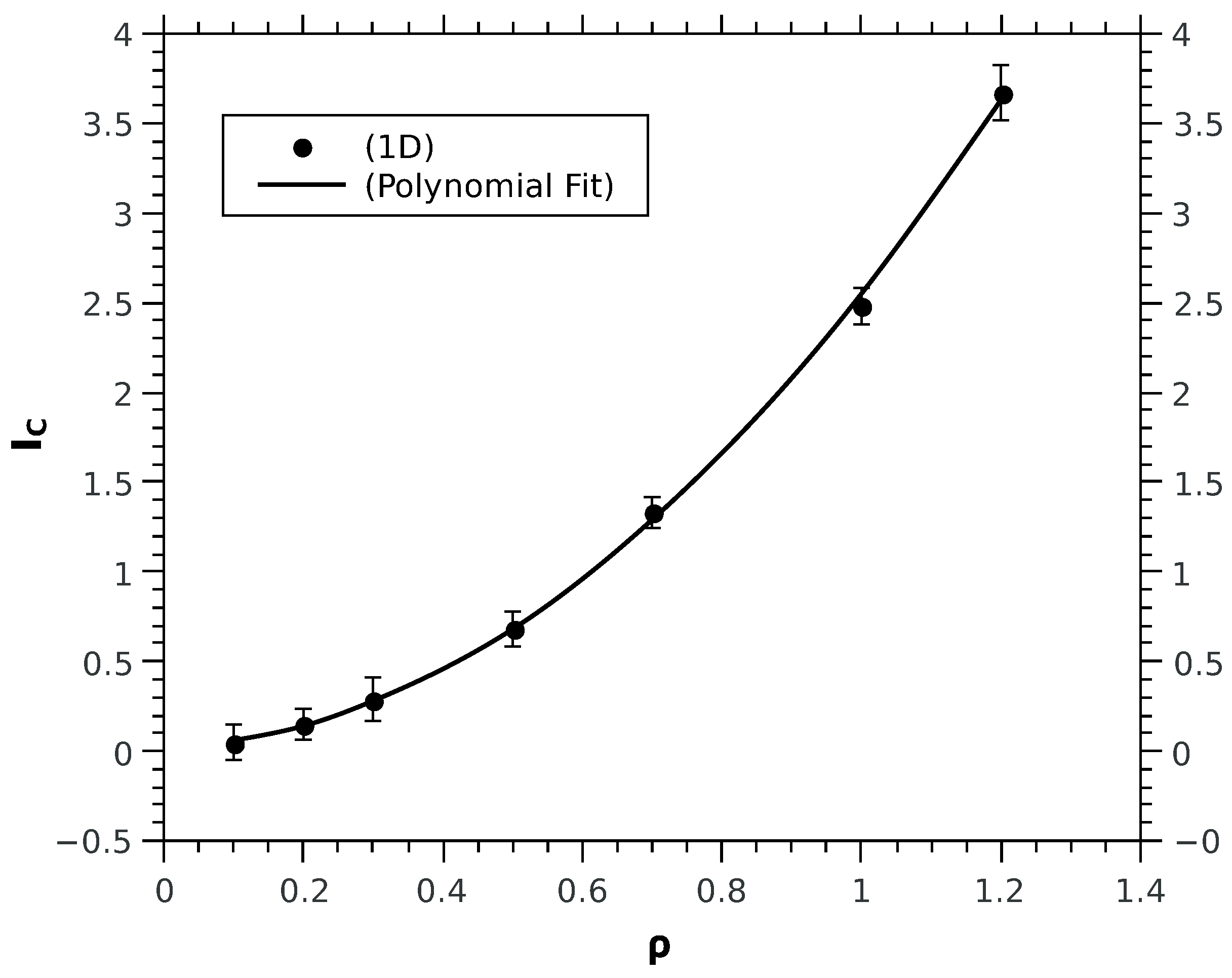
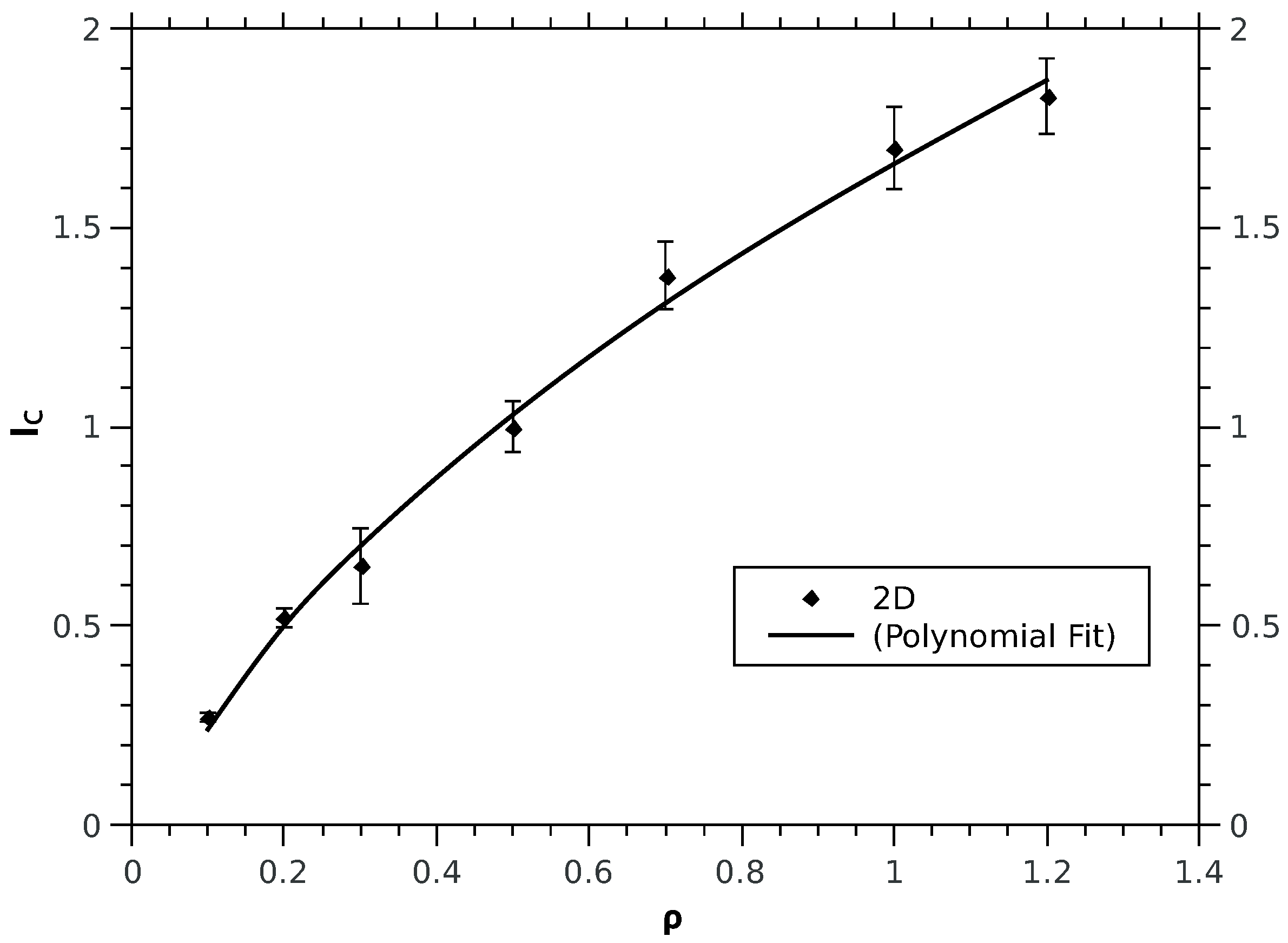
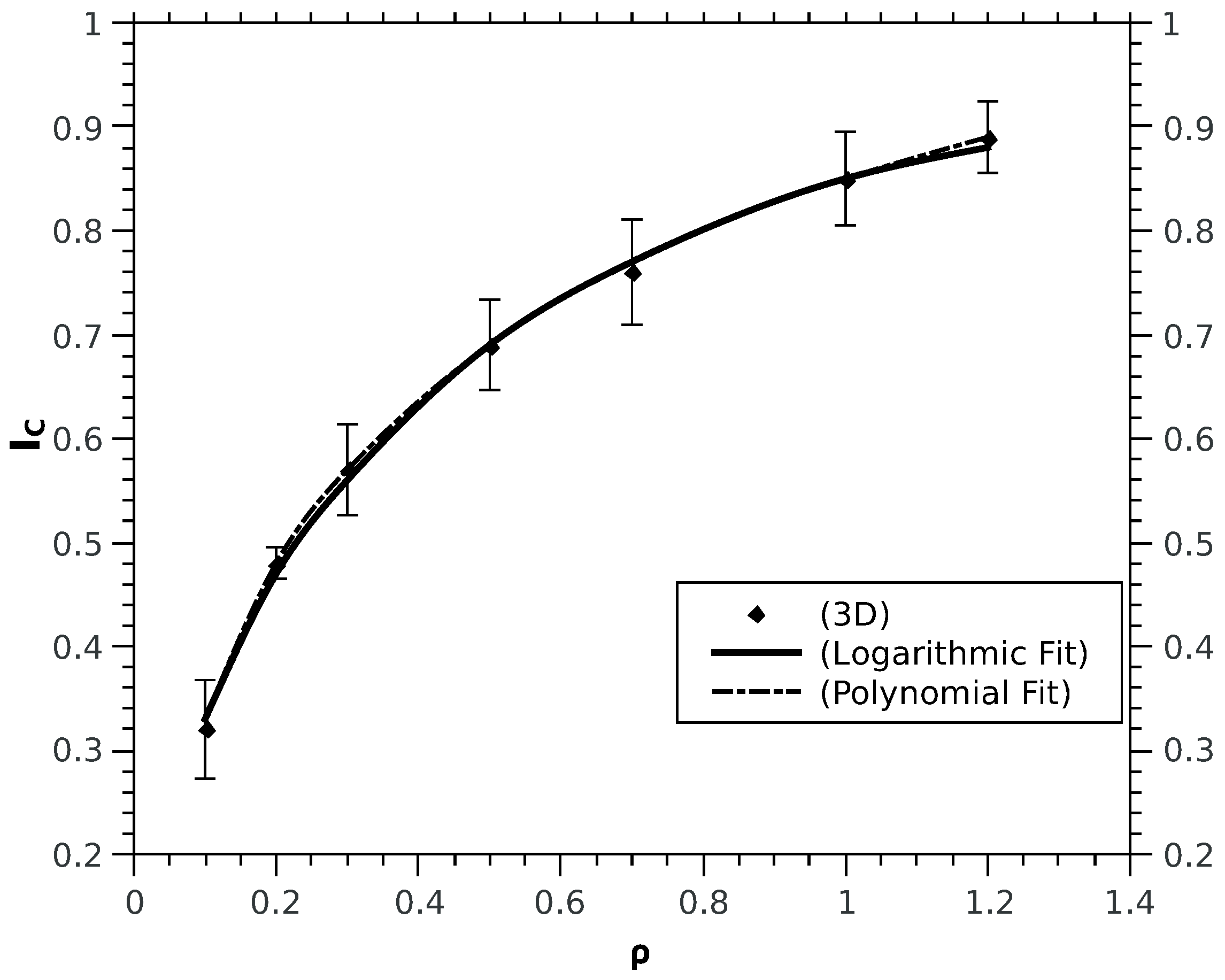
For computational convenience we treat the spinless case since the functional form of the correlation term of the kinetic functional has been shown to be independent of the explicit inclusion of the spin. We calculate for different densities in 1D, 2D and 3D; for each density a minimisation study was done to derive the corresponding optimal . The numerical values of are fitted to an analytic form. In the 1D case, is optimally fitted by a power law (see Figure 1): . For 2D and 3D cases (see Figure 2 and Figure 3): follows the analytical fits of the form, for 3D or a polynomial fitting with non integer power law: ; for 2D instead the fitting formula is: . The physical meaning of the fitting functions may turn to be very interesting from a conceptual point of view, however it does not represents the main focus of this study and will be subject of further investigations in future work; instead the change in concavity of kinetic correlation energy upon reducing the dimensions is the evident and drastic difference between the 1D case and the higher dimensions cases. The striking difference in the functional dependence of from , when comparing 1D to 2D and 3D, is the concavity: convex for 1D whereas concave for 2D and 3D. Given such a change, a question to ask is whether the role of spins, treated explicitly, may change the behaviour in 1D. Calculations with the explicit inclusion of the spin display the same power law behaviour found for the spinless case, for both the kinetic correlation and and the spin-cross correlation terms. In detail, for different k-values and within the density range, the polynomial fits for and are tabulated in Table 1 (energies and densities are in atomic units). Technical details are reported in the Appendix A.
6. Discussion
It must be stated once more that except for the assumption of the form of coupling of electrons in f, which is essentially a Jastrow factor extensively used in literature for treating correlations [30,31], the approach is then free of other assumptions. This implies that if the Jastrow factor form of f is reasonable to describe the basic physics of interacting electrons, then the behaviour of the 1D case has a real physical meaning and it is not the artifact of the assumptions of the model. In fact in 1D for both spins and spinless systems, due to the break-down of Fermi-liquid behaviour a quadratic power law has been already observed; a similar power-law scaling behaviour in 1D electron gas is also observed experimentally for properties such as conductance, tunneling current , and density of states (DOS) while in 3D the behaviour is logarithmic [25,32,33]. An additional argument in favor of a real physical meaning of our results in 1D is the fact that for the 3D case the logarithmic behaviour of found with our approach was then qualitatively verified with state of art Quantum Monte Carlo calculations [15]; in addition, in Reference [14], it has been shown that the form of f chosen leads indeed to a first-principle form of electronic correlations, meaning that is the average response in energy of the electrons to the displacement of the reference electron. It must be also reported that the conclusions of our previous work [12,13] have been strongly criticized by experts of OFDFT [34]. However the dispute was created due to a misunderstanding rather than by a conceptual or technical bug of our approach; in fact the analytic fit obtained with our approach must be considered valid only within the range of densities considered in the numerical calculations. In such a range then, the analytic fit is the closest functional form of the kinetic correlation functional (based on our sampling approach of the electron configuration in space). In this perspective the behaviour found for the 1D system in the range of densities considered and in comparison to the 3D and 2D case is worth of future attention and developments in the perspective of building valid analytic kinetic functionals.
7. Conclusions
Our results clearly suggest that the functional behaviour in 1D is different from the other two cases. The power-law behaviour with respect to the density is observed in both spin and spinless 1D cases. These results could well be related to the power law behaviour of other quantities such as conductance, current and other electronic charge properties in 1D; in fact they are nothing else than a response to a perturbation; similarly the Monte Carlo procedure of our approach at each move perturbs the system by displaying an electron in space and observes its response. The main emphasis of this study is the drastic change in the behaviour of the kinetic correlation energy (from concave to convex) going from 3D to 1D rather than the specific fitting function. It must also be clarified that the intention of this paper is not to draw final conclusion about the power law behaviour of the non analytic term (correlation term) of the kinetic functional, but to provide a basis from which to start an investigation using methods with higher accuracy. Our study at a relatively affordable computational effort serves as an indicator of a possible path of interest in the development of kinetic-energy functionals.
Acknowledgments
This work was supported by the Deutsche Forschungsgemeinschaft (DFG) with the grant CRC 1114 (project C01). We are thankful to the high-performance computing service (Zedat-HPC) at Free University Berlin for providing the computational resources.
Author Contributions
Seshaditya A. performed the computations and all the authors developed the idea. Luigi Delle Site and Luca M. Ghiringhelli designed the research plan and wrote the paper.
Conflicts of Interest
The authors declare no conflict of interest.
Appendix A. Technical Details
All Monte Carlo (MC) computations are carried out according to the protocol laid out in Reference [13]. Using Metropolis algorithm studies on the spinless system in 1D, 2D and 3D are carried out. Calculations including the effective spin-interactions (with Pauli weighing function) in 1D are also performed. To rectify the sampling problems, the spin interactions are also softened using a scaling parameter K, with values 0.5, 0.75, and 1.2. For a 3D system, cubic lattice with almost uniform electron distribution is taken as the starting configuration. A randomly selected electron is given a trial move and the move is accepted with a probability, . Periodic boundary conditions and minimum image convention are used. For different densities , the optimal parameter minimising the are obtained. In all computations, different number of electrons ( 10, 20, 30, 25, 27, 35, 64 and 100) for different densities and also same number of electrons for different densities are used (to check that the results to not depend on the number of electrons) [13]. In 3D for high densities, the evaluations are obtained using the biased MC acceptance rule due to the low value for accurate evaluations. In case of 2D and 1D, uniformly distributed electrons on a square and line are taken as the starting configurations respectively. Therefore the notion of density changes to and respectively for each case. Also in these cases, the acceptance probabilities are very low (close to 30 percent), so large number of MC samplings are used for obtaining the values.
The error bars for the kinetic-correlation energy values are computed by considering the errors in quadratic fitting of energies used for the estimation of minimum for a particular density followed by the difference in the kinetic-correlation energy values.
References
- Hohenberg, P.; Kohn, W. Inhomogeneous electron gas. Phys. Rev. B 1964, 136, B864–B871. [Google Scholar] [CrossRef]
- Wang, Y.A.; Carter, E.A. Orbital-free kinetic-energy density functional theory. In Theoretical Methods in Condensed Phase Chemistry; Schwartz, S.D., Ed.; Kluwer: Dordrecht, The Netherlands, 2002; pp. 117–184. [Google Scholar]
- Watson, S.; Carter, E.A. Linear-scaling parallel algorithms for the first principles treatment of metals. Comp. Phys. Commun. 2000, 128, 67–92. [Google Scholar] [CrossRef]
- Choly, N.; Kaxiras, E. Kinetic energy density functionals for non-periodic systems. Solid State Commun. 2002, 121, 281–286. [Google Scholar] [CrossRef]
- Chai, J.D.; Weeks, J.A. Modified statistical treatment of kinetic energy in the thomas-fermi model. J. Phys. Chem. B 2004, 108, 6870–6876. [Google Scholar] [CrossRef]
- Gavini, V.; Bhattacharya, K.; Ortiz, M. Quasi-continuum orbital-free density-functional theory: A route to multi-million atom non-periodic DFT calculation. J. Mech. Phys. Solids 2007, 55, 697–718. [Google Scholar] [CrossRef]
- Karasiev, V.V.; Trickey, S.B. Issues and challenges in orbital-free density functional calculations. Comp. Phys. Commun. 2012, 183, 2519–2527. [Google Scholar] [CrossRef]
- Wesolowski, T.A.; Wang, Y.A. Recent progress in orbital-free density functional theory. In Recent Advances in Computational Chemistry; World Scientific: Singapore, 2013. [Google Scholar]
- Levy, M. Universal variational functionals of electron densities, first-order density matrices, and natural spin-orbitals and solution of the v-representability problem. Proc. Natl. Acad. Sci. USA 1979, 76, 6062–6065. [Google Scholar] [CrossRef] [PubMed]
- Lieb, E.H. Density functionals for Coulomb systems. Int. J. Quantum Chem. 1983, 24, 243–277. [Google Scholar] [CrossRef]
- Delle Site, L. Levy-Lieb constrained-search formulation as a minimization of the correlation functional. J. Phys. A Math. Theor. 2007, 40, 2787–2792. [Google Scholar] [CrossRef]
- Ghiringhelli, L.M.; Delle Site, L. Design of kinetic functionals for many-body electron systems: Combining analytical theory with Monte Carlo sampling of electronic configurations. Phys. Rev. B 2008, 77, 073104. [Google Scholar]
- Ghiringhelli, L.M.; Hamilton, I.P.; Delle Site, L. Interacting electrons, spin statistics, and information theory. J. Chem. Phys. 2010, 132, 014106. [Google Scholar] [CrossRef] [PubMed]
- Delle Site, L. Kinetic functional of interacting electrons: A numerical procedure and its statistical interpretation. J. Stat. Phys. 2011, 144, 663–678. [Google Scholar] [CrossRef]
- Delle Site, L. Shannon entropy and many-electron correlations: Theoretical concepts, numerical results, and Collins conjecture. Int. J. Quantum Chem. 2015, 115, 1396–1404. [Google Scholar] [CrossRef]
- Garcia-Gonzalez, P. Dimensional crossover of the exchange-correlation density functional. Phys. Rev. B 2000, 62, 2321–2329. [Google Scholar] [CrossRef]
- Garcia-Gonzalez, P.; Alvarellos, J.E.; Chacon, E. Dimensional crossover of the kinetic-energy electronic density functional. Phys. Rev. A 2000, 62, 014501. [Google Scholar] [CrossRef]
- Sears, S.B.; Parr, R.G.; Dinur, U. On the quantum-mechanical kinetic energy as a measure of the information in a distribution. Isr. J. Chem. 1980, 19, 165–173. [Google Scholar] [CrossRef]
- Weizäcker, C.F. Zur theorie der kernmassen. Z. Phys. 1935, 96, 431–458. [Google Scholar] [CrossRef]
- Thomas, L.H. The calculation of atomic fields. Proc. Camb. Philos. Soc. 1927, 23, 542–548. [Google Scholar] [CrossRef]
- Fermi, E. Statistical method to determine some properties of atoms. Rend. Lincei 1927, 6, 602–607. [Google Scholar]
- Pittalis, S.; Räsänen, E. Orbital-free energy functional for electrons in two dimensions. Phys. Rev. B 2009, 80, 165112. [Google Scholar]
- Lee, R.M.; Drummond, N.D. Ground-state properties of the one-dimensional electron liquid. Phys. Rev. B 2011, 83, 245114. [Google Scholar]
- Drummond, N.D.; Needs, R.J. Phase diagram of the low-density two-dimensional homogeneous electron gas. Phys. Rev. Lett. 2009, 102, 126402. [Google Scholar] [CrossRef] [PubMed]
- Wagner, L.K.; Ceperley, D.M. Discovering correlated fermions using quantum Monte Carlo. Rep. Prog. Phys. 2016, 79, 1–9. [Google Scholar] [CrossRef] [PubMed]
- Drummond, N.D.; Needs, R.J. Quantum Monte Carlo study of the ground state of the two-dimensional Fermi fluid. Phys. Rev. B 2009, 79, 085414. [Google Scholar]
- Haldane, F.D.M. ’Luttinger liquid theory’ of one-dimensional quantum fluids. I. Properties of the Luttinger model and their extension to the general 1D interacting spinless Fermi gas. J. Phys. C Solid State Phys. 1981, 14, 2585–2609. [Google Scholar] [CrossRef]
- Astrakharchik, G.E.; Girardeau, M.D. Exact ground-state properties of a one-dimensional Coulomb gas. Phys. Rev. B 2011, 83, 153303. [Google Scholar]
- Loos, P.-F.; Gill, P.M.W. Correlation energy of the one-dimensional Coulomb gas. arXiv, 2012; arXiv:1207.0908. [Google Scholar]
- Jastrow, R. Many-body problem with strong forces. Phys. Rev. 1955, 98, 1479. [Google Scholar] [CrossRef]
- Drummond, N.D.; Towler, M.D.; Needs, R.J. Jastrow correlation factor for atoms, molecules, and solids. Phys. Rev. B 2004, 70, 235119. [Google Scholar]
- Deshpande, V.V.; Vikram, V.; Bockrath, M.; Glazman, L.I.; Yacoby, A. Electron liquids and solids in one dimension. Nature 2010, 464, 209–216. [Google Scholar] [CrossRef] [PubMed]
- Kukkonen, C.A.; Overhauser, A.W. Electron-electron interaction in simple metals. Phys. Rev. B 1979, 20, 550–557. [Google Scholar] [CrossRef]
- Trickey, S.B.; Karasiev, V.V.; Vela, A. Positivity constraints and information-theoretical kinetic energy functional. Phys. Rev. B 2011, 84, 075146. [Google Scholar] [CrossRef]
Figure 1.
Computed values of for different densities in 1D obtained at optimal values. The analytical fit in this case is with RMS error value 0.0165. All values are in atomic units.
Figure 1.
Computed values of for different densities in 1D obtained at optimal values. The analytical fit in this case is with RMS error value 0.0165. All values are in atomic units.

Figure 2.
Computed values of for different densities in 2D obtained at optimal values. The Polynomial fit in this case is: with error 0.0277. All values are in atomic units.
Figure 2.
Computed values of for different densities in 2D obtained at optimal values. The Polynomial fit in this case is: with error 0.0277. All values are in atomic units.

Figure 3.
Computed values of for different densities in 3D obtained at optimal values. The analytic fit obtained in this case, and the polynomial fit is given by with RMS values 0.0273 and 0.0324 respectively. All values are in atomic units.
Figure 3.
Computed values of for different densities in 3D obtained at optimal values. The analytic fit obtained in this case, and the polynomial fit is given by with RMS values 0.0273 and 0.0324 respectively. All values are in atomic units.


Table 1.
Polynomial Fits for and values (with RMS errors in parenthesis) for 1D including the spin.
| k Value | ||
|---|---|---|
| k = 0.5 | ||
| k = 0.75 | ||
| k = 1.2 |
© 2017 by the authors. Licensee MDPI, Basel, Switzerland. This article is an open access article distributed under the terms and conditions of the Creative Commons Attribution (CC BY) license (http://creativecommons.org/licenses/by/4.0/).
Share and Cite
MDPI and ACS Style
A., S.; Ghiringhelli, L.M.; Delle Site, L. Levy-Lieb-Based Monte Carlo Study of the Dimensionality Behaviour of the Electronic Kinetic Functional. Computation 2017, 5, 30. https://doi.org/10.3390/computation5020030
AMA Style
A. S, Ghiringhelli LM, Delle Site L. Levy-Lieb-Based Monte Carlo Study of the Dimensionality Behaviour of the Electronic Kinetic Functional. Computation. 2017; 5(2):30. https://doi.org/10.3390/computation5020030
Chicago/Turabian StyleA., Seshaditya, Luca M. Ghiringhelli, and Luigi Delle Site. 2017. "Levy-Lieb-Based Monte Carlo Study of the Dimensionality Behaviour of the Electronic Kinetic Functional" Computation 5, no. 2: 30. https://doi.org/10.3390/computation5020030
Note that from the first issue of 2016, this journal uses article numbers instead of page numbers. See further details here.