
Introduction to Advanced X-ray Diffraction Techniques for Polymeric Thin Films

Department of Physics, University of Colorado, Boulder, CO 80309, USA
Coatings 2016, 6(4), 54; https://doi.org/10.3390/coatings6040054
Submission received: 30 June 2016
/
Revised: 24 September 2016
/
Accepted: 24 October 2016
/
Published: 1 November 2016
(This article belongs to the Special Issue Polymer Thin Films)
Abstract
:X-ray diffraction has been a standard technique for investigating structural properties of materials. However, most common applications in the organic materials community have been restricted to either chemical identification or qualitative strain analysis. Moreover, its use for polymeric thin films has been challenging because of the low structure factor of carbon and the thin film nature of the sample. Here, we provide a short review of advanced X-ray diffraction (XRD) techniques suitable for polymeric thin films, including the type of analysis that can be done and measurement geometries that would compensate low signals due to low carbon structure factor and the thin film nature of the sample. We will also briefly cover the -pole figure for texture analysis of ultra-thin film that has recently become commonly used. A brief review of XRD theory is also presented.
Keywords:
thin film; polymer; XRD; X-ray; organic photovoltaics; organic electronics; structure; GIXD1. Introduction
Polymer thin films are ubiquitous in contemporary life. Most commonly, they can be found as protective or optical coatings, but the last few decades has witnessed the birth of organic electronics, thus furthering incorporation of polymer thin films into cutting edge technologies and exponential growth of the field. Whether a film is utilized for its optical, electronic, chemical, or surface properties, in-depth understanding of its structural properties is often crucial to development of a successful product. This is because (1) all of these four properties are intertwined, and (2) the thin nature of these films—typically a few nanometers to a few microns—fundamentally leads to a significant constraint to material growth, impacting its other properties as compared to the bulk material. This is especially true for polymeric ultra-thin films, where the size of the building blocks of the film, a polymeric chain, can be of the same order of magnitude as the film thickness itself.
X-ray diffraction (XRD) is the most well-known family of techniques to investigate structural properties of a material. Traditionally, XRD is employed on thick or powdered materials because of its penetration depth and thus its ability to reveal internal structural properties of the material. On the other hand, thin films structural properties are often investigated by surface characterization techniques (e.g., atomic force microscopy), approximating the internal structure as being similar to the surface structure. However, this may not be true. For example, vertical phase segregation and structural changes have been seen in organic ultra-thin films [1,2,3,4], emphasizing the necessity for a thorough investigation.
Using XRD on polymer thin films for analyses beyond chemical identification, however, is not without its challenges. There are four main challenges, and the first three are technical: (1) low atomic number of carbon—the main building block of organic materials—leading to low X-ray scattering intensity, (2) thin film nature of the sample which amplifies the first problem of low signal intensity, and (3) sensitivity of some samples to room atmospheric condition, which if applicable, will further exacerbate the first problem. Lastly but most importantly, polymeric systems are much more complex than inorganic systems at the molecular level. Therefore, we need (4) correct interpretation of the XRD data.
In this article, we will cover three main topics. First, we briefly review the structural anatomy of a typical sample and make a connection to what is measurable by XRD. Second, we will briefly review the basics of XRD and identify which structural properties are accessible to this family of measurement techniques. Lastly, we will discuss advanced XRD techniques that have been utilized to measure these structural properties, while paying special attention to the four problems indicated earlier. This article is tailored to giving a brief introduction of these techniques to an investigator who is new to the field. This introduction and the first section should also serve to brief an experienced inorganic material XRD investigator with the nuances unique to organic materials. As such, we omit the finer details, and focus on delivering the concepts and important equations. The motivated readers are encouraged to further read the references for more in-depth discussions.
2. Structural Anatomy of Materials
Any material can be modeled as a mixture of both ordered and disordered parts; the largely ordered parts of the the material are called crystal(lites) and the largely disordered parts are called amorphous. Naturally, the focus of any investigation on structural properties of a material is measuring the degree of order or disorder in the atomic placements inside the sample. In this section, we will briefly review these concepts and how they extend to polymeric systems.
There are three important quantities of interest when quantifying how ordered a material is: what crystallites are present in the sample, how much of the sample comprises of such crystallites, and how the crystallites are oriented in the sample.
In a crystallite, atoms are spatially placed in a regular interval called the crystal’s “lattice parameters”. In three-dimensional crystals, these are comprised of a set of three lattice vectors (a, b, c) and 3 angles (, , ) (Figure 1a) [5,6]. Lattice parameters are the most important physical quantity in XRD as periodicity in atomic placement is the physical property that gives rise to XRD peaks. Additionally, the set of lattice parameters is unique to every crystal composition. For example, lattice parameters for NiO crystal is different from that of Ni or . This makes measuring lattice parameters useful for compositional analysis, one of the most common application of XRD. Additionally, if a material is under mechanical stress, the lattice parameters may also slightly change, allowing us to detect macrostrains inside a sample.
To extend this concept to organic systems, note that lattice parameters are not required to repeat across nearest neighbor atoms. In the simplest case, pairs of atoms separated two lattice parameters away will create harmonics (higher diffraction order) in the XRD signal, just like in optical diffraction. Naturally, this also means that if large organic molecules or chains are highly ordered, they will necessarily produce XRD signals. It is important to note, however, that in organic systems, an XRD signal is not necessarily correlated with optical signature. While the former involves long-range structural order, the latter typically requires only inter-molecular aggregates. References [3,7,8,9,10,11,12,13,14] provide in-depth examples of such advanced X-ray studies on polymeric samples.
In a single crystal, the whole material is part of a single lattice. However, in most cases, a material is composed of a mixture of many crystallites, large or small, and amorphous regions (Figure 1a). The more crystallite the material contains, the higher its degree of crystallinity is. Degree of crystallinity is often of practical interest because it is very tightly related to a material’s electrical conductivity, optical properties, and mechanical properties. Crystallite size also varies from a few nanometers in size to large slabs in centimeters. As XRD signal intensity depends on the the number of atoms that are part of the crystalline structure, both degree of crystallinity and average crystallite size are accessible through careful analysis of XRD data.
Another important structural characteristic is called the crystallographic “texture”, which measures the orientation of the crystallites in a sample (Figure 1b). By definition, a single crystal must have perfect texture. Similarly, an epitaxial film will have a near-perfect texture, and a perfect polycrystalline film will contain randomly-oriented crystallites. There also exist samples which fall in the middle of this textural spectrum, consisting of some crystallites which are highly oriented, and some randomly-oriented crystallites. There are also materials that are uniaxially textured: its crystallites are oriented only in one direction. Naturally, textured materials tend to exhibit non-isotropic electrical, optical, and mechanical properties. A relevant example is anisotropy of electrical conductivity commonly found in conjugated polymer thin films, which has been attributed to its semi-ordered nature [8,16,17]. On the other hand, non-textured materials tend to have isotropic properties. Quantification of sample texture can be done with XRD using “pole-figures”.
Let us now briefly conceptualize structural disorder in materials. Like crystallinity, structural disorder of any kind alters properties of materials and may lead to interesting physical phenomena. For example, structural disorder contributes to electrical conduction in otherwise ideally insulating materials [18,19], is central in photoconductivity [19], and reduces the conductivity of crystalline semiconductor. Likewise, disorders also affect opto-electronic properties of organic polymers [3,8,20,21]. Being able to quantify these disorders in a systematic way is therefore of interest.
Structural disorder in the context of XRD is usually discussed in terms of average atomic displacement from its ideal crystalline position. The most coarse way to categorize structural disorder is to divide them into non-cumulative and cumulative disorder [10]. Non-cumulative disorders refer to cases in which the atoms’ dislocation does not depend on their locations in the crystal. In effect, this means that such disorder does not significantly disrupt crystal formation. Physical examples include disorder due to thermal energy where the dislocation tends to follow Gaussian distribution at random directions, or fault dislocations in a crystal slab. This kind of disorder broadens XRD peaks and reduces their height but has no other effect.
On the other hand, in a cumulative disorder, there is a positional dependence in the atomic displacement from the ideal position: . A physical example is the disorder caused by impurity atoms with significantly different size than the primary atoms [15]. Unlike non-cumulative disorder, this type of disorder propagates across the whole crystallite, severely disrupting the crystal structure. Cumulative disorder will affect both peak shape and height as a function of diffraction order.
Lindenmeyer, Beumer, and Hosemann, in the context of the paracrystal theory, suggested that we divide the cumulative disorders in a mathematically systematic way into [15]:
- non-cumulative disorder (e.g., disorder due to thermal excitation, fault dislocation);
- cumulative (paracrystalline) disorder,
- inter-crystal disorder (),
- inter-plane disorder (, part of intra-crystal disorder),
- intra-plane disorder (, part of intra-crystal disorder),
Inter-crystal disorder can be thought of as the micro-strain contribution to the disorder. The combination of the first two terms form the total paracrystallinity in the absence of intra-plane disorders and can be assessed by XRD via Warren–Averbach (peak-shape) analysis. This involves analyzing the peak shape of multiple harmonics of XRD peaks, which may also give an estimate for mean crystallite size [21,29,30].
The last term, on the other hand, is neglected in the ideal paracrystal theory. While in essence this quantity should manifest in XRD data, at the time of this writing, the author has not encountered an XRD experimental result that clearly separates intra-plane disorders from the other two disorders and therefore this topic is outside the scope of current discussion. However, we remark that in polymeric systems, e.g., poly-3-hexyl-thiophene (P3HT), this quantity is understood to be inter-atomic disorders within the polymer chain, which is very closely related to their optical absorption spectrum [31,32,33,34,35]. From this point of view, it should not be surprising if the disorder observed via available XRD data are not correlated with those observed via optical absorption spectroscopy: although a crystalline material implies aggregation, the converse may not be true. In the same light, we strongly agree with the suggestion made by Duong et al. [17] to strictly differentiate “crystallite” from “aggregate”, and “crystalline” from “aggregated”.
3. Review X-ray Diffraction Theory
XRD signal is a result of an elastic scattering of monochromatic X-ray by core electrons of atoms in a sample. The regularly-spaced atoms in a crystal lattice causes the X-rays to be diffracted, producing the well-known XRD patterns, analogous to diffraction of visible light by gratings. Mathematically, XRD signal is best-known to follow Bragg’s Law for constructive interference (Figure 2a):
where d is the separation between the Bragg planes, is the Bragg angle, m is the diffraction order, and is the X-ray wavelength. The term Bragg planes refers to planes that are comprised of these constructively diffracting atoms. In the simplest case, the measured d equals the magnitude of one of the lattice parameters, allowing us, for example, to identify chemical identity of the sample. Furthermore, in inorganic materials, the lattice parameters are usually equal to the spacings between neighboring atoms. However, as illustrated in Figure 1a, this last point is usually not true in organic systems.
To facilitate our discussions on the advanced XRD techniques suitable for thin film samples, we need to take a more general approach and derive the condition for interference vectorially. This mathematical representation will greatly help us when we discuss sample texture, diffraction at grazing incidence, and diffraction with 2D detector.
Consider two atoms separated by a displacement vector (Figure 2b). A monochromatic light of wavelength is incident on them along the direction . Its wavevector is . The lights are scattered by the scatterer in the direction . Because the scattering is elastic, the magnitude of the outgoing wavevector and its wavelength remain constant. The condition for constructive interference is that the phase difference of the two light paths is an integral multiply of . From Figure 2a, the condition for constructive interference is:
where the integer m is called the diffraction order. When , the quantity is exactly the shortest reciprocal lattice vector, , of the diffracting crystallographic planes, and its magnitude is simply:
and the condition for diffraction (Equation (2)) can be re-written as:
This equation and Figure 2c summarize the criteria for constructive interferrence. This equation carries a few physical significances about the condition for XRD signal: since the magnitudes of and are the same, is simply the bisector of the angle subtended by them. It follows that and must make the same angle to a plane perpendicular to . Therefore the photon scattering event can be seen as a Bragg reflection off this plane with Bragg angle . Note that the direction of must also equal that of . Qualitatively, this leads to two ramifications: first, note that the magnitude of changes as changes. This means that changing leads to a different set of Bragg planes with different d (Figure 2d,e). Naturally, since , changing a X-ray wavelength will also change . Second, since q is a bisector of the incoming beam () and outgoing beam (), we are able to sample Bragg planes that are not parallel to the sample surface by changing incidence/exit angle (Figure 2f). This last point will be particularly important in XRD experiments involving geometries other than Bragg–Brentano.
Lastly, the connection with Bragg’s Law (Figure 2a) can also be made with the help of Figure 2c. From Figure 2c, the magnitude of is simply . From Equations (2) and (3), this also equals . Using the definition of wave vectors, we finally arrive at the usual formulation for Bragg’s condition:
Likewise, the magnitude of is related to by:
Note that q is one of the most commonly used variable in the field of XRD.
Thus far, we have only touched upon locations of the XRD peaks that give us information about d. On the other hand, analyzing XRD peak shape allows us to quantify the degree of structural disorder in the sample. The most widely-used analysis method to extract this information is by analyzing the Fourier coefficient of the peak shapes of multiple diffraction orders, the Warren–Averbach analysis [29]. Note that this type of peak-shape analysis is done on XRD signals as a function of q. Neglecting the structure factor, it can be shown that the Fourier coefficients of XRD peak shapes of diffraction order m can be factored into size-, non-cumulative disorder-, and cumulative-disorder-dependent terms, , , and , respectively [10,22,30]:
where
Here, S is the average number of diffraction planes in a crystallite ( is the average crystallite size), g is the average paracrystallinity [26], and is the average non-cumulative displacement from ideal sites. The function describes the distribution of the number of diffraction planes in a crystallite. In the simplest case, it can be modelled as a delta function , but, more realistically, a gamma function centered around S should be used.
From Equation (7), we can draw the following conclusions: (1) peak shape and height are dependent on diffraction order, (2) crystallite size governs the overall peak height while disorder reduces the peak height via peak broadening, (3) non-cumulative disorder contributes to a Gaussian peak shape, while (4) paracrystalline disorder contributes to a Lorenzian peak shape. Therefore, in the absence of significant alteration due to beam optics, we expect that (5) the overall XRD peak shape is Voigt.
4. X-ray Diffraction Techniques for Polymer Thin Films
When planning for an XRD experiment on organic thin films, one needs to consider three questions: (1) if there is a necessity to use a synchrotron, (2) what quantities are going to be analyzed, and (3) what measurement geometry should be used.
The first question is rather unique to organic thin films. Organic materials such as polymers have much lower diffraction strength compared to similar inorganic samples at the same X-ray flux. Combine this with the thin nature of our samples, and we are posed with the necessity for very long data integration time. Lab-scale X-ray systems are typically not bright enough for a timely high-quality data collection of organic samples thinner than ∼100 nm regardless of measurement geometry, and, therefore, a synchrotron-based experiment is usually required. Thicker samples can be measured with lab-scale systems, although they often need to be measured in grazing-incidence geometries for best results. Additionally, depending on the sample, the investigator often need to weigh in possible sample damage due to X-ray radiation or exposure to ambient air. An inert measurement chamber is typically used to reduce potential degradation in ambient air, while translating the sample stage in between measurements has been used to reduce X-ray damage to the sample.
There are three quantities that can be analyzed: (1) peak location, (2) peak intensity, and (3) peak shape. From Bragg’s law, peak location gives information on lattice constants and can therefore be used to examine chemical composition or crystal symmetry. Peak intensity is related to the amount of crystallites that are reflecting X-rays into the detector (i.e., crystallites with correct orientation) and may shed light on, for example, degree of crystallinity. The dependence of peak intensity on the crystallite orientation will also be important in investigating crystallographic texture of the sample. Lastly, peak shape is a convolution of various factors such as crystallite size, strain, and paracrystallinity. It is therefore related to, but not exclusively, the degree of disorder in the material. Note that peak shape analyses typically require multiple harmonics of the XRD peak of interest and therefore require ample X-ray dosing and high resolution.
Most measurements on organic thin films have been focusing on chemical identification, degree of crystallinity, macrostrain, and material texture, and therefore only involve the first two quantities. However, in-depth analysis on the peak shape to quantify structural disorder has been performed [10].
There are various X-ray measurement geometries, suitable for different slices of X-ray data and sample geometry. In this section, we will discuss only X-ray measurement geometries that are applicable to polymer thin films, their strength, special correction factors, and brief application examples. These measurement geometries are different in terms of the following:
- Incident () and exit angles (, ) of the X-ray;
- Angle that is scanned (changed as a function of time);
- Detector geometry (point vs. 1D vs. 2D).
To facilitate our discussion, the measurement angles are explained in Figure 3.
The basic rules on measurement geometry are as follows: (1) From Bragg’s Law, changing the difference in X-ray angles determines the lattice constant that is being sampled. On the other hand, (2) changing the X-ray angles with respect to the sample angles determines which crystallite orientation is being sampled and will be useful in determining sample texture. (3) Consider the goniometer axes’ range and precision when choosing the goniometer angle that is to be scanned. Rotate the sample if necessary. (4) Lower incident angle means higher sampling area, possibly lower background signal from the substrate, and reduced beam damage on the sample. While this is appropriate for thin films, it comes with significant trade-offs that will be discussed in the subsequent subchapters. Lastly, (5) when variable wavelength X-ray source is available, consider optimizing the wavelength for your application.
4.1. Common Peak Intensity Corrections and Background Subtraction
When analyzing XRD peak intensity and peak shape, it is important to apply the relevant intensity corrections and do background subtraction. While most of these corrections depend on the geometry of the measurement system, the following two correction factors are not geometry-dependent (peak intensity is to be divided by correction factor). Additional corrections specific to special measurement configurations will be discussed in the appropriate subsections.
The first correction factor is the scattering factor of different atoms. Higher atomic number corresponds to a higher number of electrons and thus higher X-ray scattering intensity. For most polymeric systems, this factor is not very important since most of the scattering centers are carbon. However, it does explain why polymeric systems have low X-ray peak intensity. Should one deals with analysis of Bragg planes that consist of other elements, and the table for atomic scattering factor as a function of atomic number and X-ray energy can be found in most synchrotron resources.
The second correction factor is applicable to X-ray sources that are partially polarized. When the X-ray source is partially polarized, the following polarization correction needs to be applied:
where is the fraction of light that is polarized parallel to the sample surface, is the exit angle perpendicular to the sample surface, and is the exit angle parallel to the sample surface (Figure 3). Lab-scale sources tend to be randomly polarized, while synchrotron radiation tends to be highly polarized.
For further reading, references [36,37,38] discuss these corrections in great detail and touch upon a few other corrections that may be important for other material systems.
Background signals may arise from diffuse scattering from the air along the beam path or the sample substrate [37]. While this can be very complex to model, in most cases the background as a function of q can be sufficiently fitted with a decaying exponential function at low q and power function at higher q. Note that when multiple peaks are present, all peaks and the two background functions must be fitted simultaneously. The isolated peak, therefore, equals the signal minus the background and all other peaks.
4.2. Bragg–Brentano Geometry
The most commonly used XRD measurement geometry is called Bragg–Brentano geometry. In this technique, is fixed at zero while and are scanned equally. Figure 2a illustrates this geometry (note that always equal in this geometry). This way, the angle between and is always equal 2, allowing us to easily identify the lattice constant.
Because , Bragg–Brentano geometry only samples Bragg planes whose norm is perpendicular to (Figure 2a,d,e). This means that if the sample is textured and the crystallites are facing other directions (or slightly misoriented), the peak height may be dramatically reduced or the measurement may not even pick up any signal at all, potentially leading to a false negative if not done carefully. Some measurement techniques introduced in the next subsections will address this major disadvantage.
Another important point regarding analyses on measurement results from Bragg–Brentano geometry is that when analyzing XRD data involving a scan in , the Lorentz correction need to be applied:
This correction takes into account the amount of time each diffracting crystallite remains in the diffracting position, thus correcting for the different integration time of different Bragg angles [36,39]. Usually, this correction factor combines with the polarization correction and is collectively known as the Lorentz-polarization factor. However, it is important to note that, unlike the polarization correction, the Lorentz correction will change the shape of diffraction peaks due to its -dependence and is therefore important in peak shape analyses.
When all correction and background subtraction has been properly applied, Bragg–Brentano geometry is suitable to be used for peak shape analysis. The general procedure for Warren–Averbach analysis goes as follows: first, high quality data where multiple peaks are clearly resolved with ample data points are taken (Reference [10] suggests at least 100 data points over full-width-at-half-max).
Proper correction and background subtraction is then applied to the data. Equation (7) is then simultaneously fitted to the Fourier transform of multiple isolated XRD peaks. Note that each peak will have different diffraction order m and that the fit must be done simultaneously across all peaks. Estimation of crystallite size in the direction normal to the sample (i.e., in ), rms non-cumulative disorder, and the degree of paracrystallinity can then be obtained from the fit results. Reference [10] provides a rigorous example of Warren–Averbach analysis to quantify disorder in organic films. A more basic example on clays is explained in Reference [30]. Furthermore, Reference [10] also demonstrates the utilization of pseudo-Voigt fit to get a qualitative understanding of the various disorders in the sample.
4.3. Pole Figure
When the sample is textured, it is often essential to be able to quantify the distribution of crystallite orientation. For example, if one wishes to accurately measure XRD peak height or shape, in general, one needs to first find the direction of the reference Bragg planes, and then precisely orient the sample such that is perpendicular to the Bragg planes before starting the measurement.
A pole figure is a visualization of the distribution of crystallite orientations in the sample, made by rotating the sample axes ( and ) while fixing and corresponding to the Bragg reflection of interest. Take, for example, a pole figure of a Si (111) planes from a <100> wafer. To produce the pole figure, we first set the sample and goniometer in Bragg–Brentano geometry, but with fixed at the value corresponding to Si (111) planes (this value is dependent on the X-ray wavelength. For the commonly used sources, ). Instead of scanning , we will now rotate , and incrementally increase . In this way, we essentially map all directions at which Si (111) crystallites in the sample are oriented. Because of the crystal symmetry, we will only see data at four points at . This, and examples of how the data should look for a few other cases are shown in Figure 4c. The figures also illustrate the effect of the background from an amorphous substrate (e.g., glass), which will be common when investigating a polymeric thin film because, most likely, the X-ray would penetrate the sample.
A pole figure is important in investigation of organic materials considering the low symmetry of the material; however, sometimes there is a high chance of uni-axial texture due to the preferred orientation in molecular packing. This method, for example, has been used to show that certain deposition conditions of poly-3-hexylthiophene (P3HT) may result in highly-textured nanofilms with high electronic transport properties along the substrate plane [9].
4.4. Glancing Incidence X-ray Diffraction (GIXD)
Thin organic materials, including polymeric thin films, pose a rather unique challenge to X-ray experiments. The low scattering factor of carbon combined with the low sample volume in thin film samples often means long measurement time. This is especially true for sub-micron films. In cases where the polymeric film is not chemically stable (e.g., degradation in ambient atmosphere, or X-ray damage), measurement time can be a very important consideration. The most direct workaround is to enclose the sample in an inert chamber or to modify the beam intensity. Another way to tackle this issue is by modifying the measurement geometry.
Grazing Incidence XRD, or Glancing Incidence XRD (GIXD) refers to an XRD measurement done with a fixed, very low incidence angle . In the case of measurements with 1D detectors, the detector arm may be scanned out of the sample plane or in the sample plane. This measurement geometry is particularly useful for increasing signal yield by increasing the irradiated volume, especially in the case of thin film samples. It also has the added benefit of reducing irradiated substrate volume.
In the simplest case, this added benefit can be explained using pure geometry. Consider a sample that is thinner than the absorption length of the X-ray (∼m), and that the X-ray is incident at a high angle (Figure 5a). In this case, potentially a large portion of the incident X-ray is actually absorbed by the substrate rather than the sample, leading to signal loss. Reducing the incident angle will allow more X-rays to be absorbed by the sample rather than the substrate, thus increasing signal yield. Additionally, the X-ray flux on the sample is also reduced as the X-ray is now spread over a larger sample area, reducing X-ray damage.
Another important consideration when measuring GIXD is the critical angle for total X-ray external reflection on the sample, which is typically a very low angle, around the range of incident angle of interest. Below this angle, X-rays will be totally reflected off the sample surface and will only couple with the sample through the evanescent (waveguide) modes. Therefore, setting the incident angle above and below the critical angle will further allow the investigator to sample from, respectively, the “bulk” of the thin film sample or just the surface.
When combined, these benefits may reduce data collection time by orders of magnitude, while reducing beam damage on the sample. However, there are a few additional subtleties related to interpreting and post-processing GIXD data that need to be addressed [38,40,41]:
- Due to the fixed incidence angle, the orientation of the Bragg planes is necessarily different for different ,
- Blind area due to forbidden Bragg reflection;
- Absorption correction which depends on film thickness, increased irradiated area, and the position of the sample;
- Shift in measured due to refraction.
The first point can be understood with the help of Figure 2c while fixing the incoming angle. Let be fixed, and the magnitude of be varied. As discussed in the previous section, the conditions for constructive interference require (1) magnitude of equal to that of , and (2) being the bisector of and . In order to satisfy both conditions, the direction of must swing closer to as its magnitude increases. Since also points in the direction of the diffracting crystallites, it follows that the orientation of the crystallites that are being sampled, and, therefore, the associated Bragg planes must also be different for different .
The second point is related, but important only when investigating texture of the film. Suppose that we restrict the incoming angle at a low angle , and investigate a fixed q (Figure 5). Equation (4) dictates that a diffraction spot will only be produced when orientation of the crystallite is parallel to . Remember that always bisects the incoming and outgoing beam. Suppose the outgoing beam does not deviate left or right (). Then, will be akin to in Figure 5c. Likewise, if the outgoing beam is parallel to the sample surface, it will be like in Figure 5c. Directions of vectors and represent the extreme crystallite orientation that can be sampled at a fixed . Note that any that lies inside the cone subtended by is not within these extremes. In other words, crystallites whose orientation lies within the cone from the normal will never satisfy Equation 4 and gives no diffraction peak. In the limit that , the validity limit of the data becomes [9].
The absorption correction corrects for the change in scattering volume due to the geometrical effects. It depends on film thickness and is important for thin films (intensity data are to be divided by the correction factors):
where and are the incidence and exit angles (Figure 3), t is the film thickness, and is the extinction coefficient of the X-ray in the material. In the case where the sample size is finite, the beam may spill over and diffraction intensity is limited by the sample size. Intensity might also be limited by the effective detector size, which is set by the X-ray optics.
The last correction is important when is close to the critical angle for total internal reflection of the X-ray inside the sample. At an incidence angle close to the critical angle for total external reflection of the X-ray, the position of the measured Bragg angle shifts by a few tenths of a degree to a smaller angle due to refraction [41]:
where is the critical angle for total external reflection of X-ray, and is the imaginary part of the material’s index of refraction.
This technique has become more frequently used in organic film samples [3,9,10] because it greatly compensates for the low structure factor of carbon. However, the fact that in this geometry the direction of varies makes it unsuitable for rigorous peak-shape analysis unless it is known that the sample is not textured.
4.5. GIXD and Pole Figure with a 2D-Detector
Another way to greatly improve measurement time is by replacing the point detector with a two-dimensional detector [42], which offers much more information at the expense of resolution. Unlike in inorganic materials, polymeric thin films tend to exhibit broad peaks, so lower data resolution is often not a limiting factor. Furthermore, data resolution can be improved at the expense of data range by moving the detector closer to the sample. Since the main interest in the polymeric thin film community is typically limited to phase identification, texture, and semi-quantitative analysis of degree of crystallinity, GIXD with a 2D-detector is often the preferred way of doing XRD on thin polymeric films. Much of the development of this technique has been in support of the organic semiconductor community [12,13,14]; nevertheless, undoubtedly the techniques and analysis methods are readily applicable to any polymeric thin films.
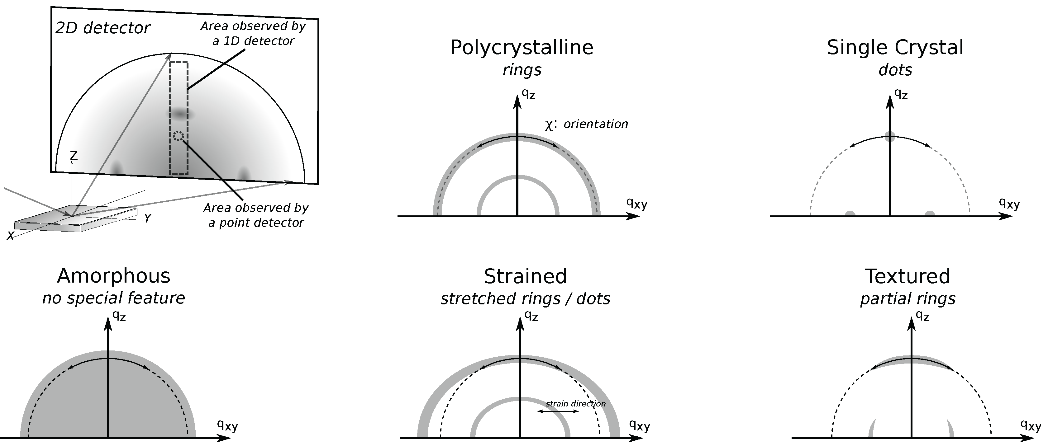
Figure 6 illustrates the richness in XRD data taken using a 2D-detector, which takes a “picture” of the XRD pattern (Debye rings). Data taken using lower-dimension detectors are essentially a subset of the data taken using a 2D detector. In 2D XRD data, radial direction is the direction of increasing , while the azimuthal direction is much like in pole figures. However, because of the forbidden Bragg reflection (“hole”) in GIXD discussed in the previous subsection , the direction perpendicular to sample norm on the detector corresponds to instead of , and additional specular data is needed if one wishes for data from this forbidden -range.
Sample texture is readily assessed from 2D GIXD data (Figure 6). For example, a perfect polycrystalline sample displays full Debye rings, while single crystals appear as dots. Likewise, data from samples with texture somewhere in-between these extremes will appear as partial rings and macrostrains readily result in a shifted dot or a stretched ring in 2D XRD data. On the other hand, data from amorphous materials will be lacking any special feature.
Three points are worth mentioning about this measurement geometry. First, like in the case of GIXD, since the incidence angle is fixed, the different Bragg reflections (different or ) must necessarily come from Bragg planes with different orientation. This means that 2D detectors should not be considered as a silver bullet for examining structural properties of highly-textured samples such as single crystals. In such cases, the chance of missing data is still very high if the sample is misoriented. Second, since the image detectors are usually flat while diffraction is spherically symmetric, there is a non-linear relationship between (or ) and pixel position on the detector. A correction can be applied when proper calibration is done as per Reference [43]. Lastly, this also means that (or ) resolution of the detector also changes radially, with the highest resolution achieved at the positions furthest from the detector origin. Consequently, the sample-detector distance can be adjusted to get the optimum resolution for the -range of interest [43].
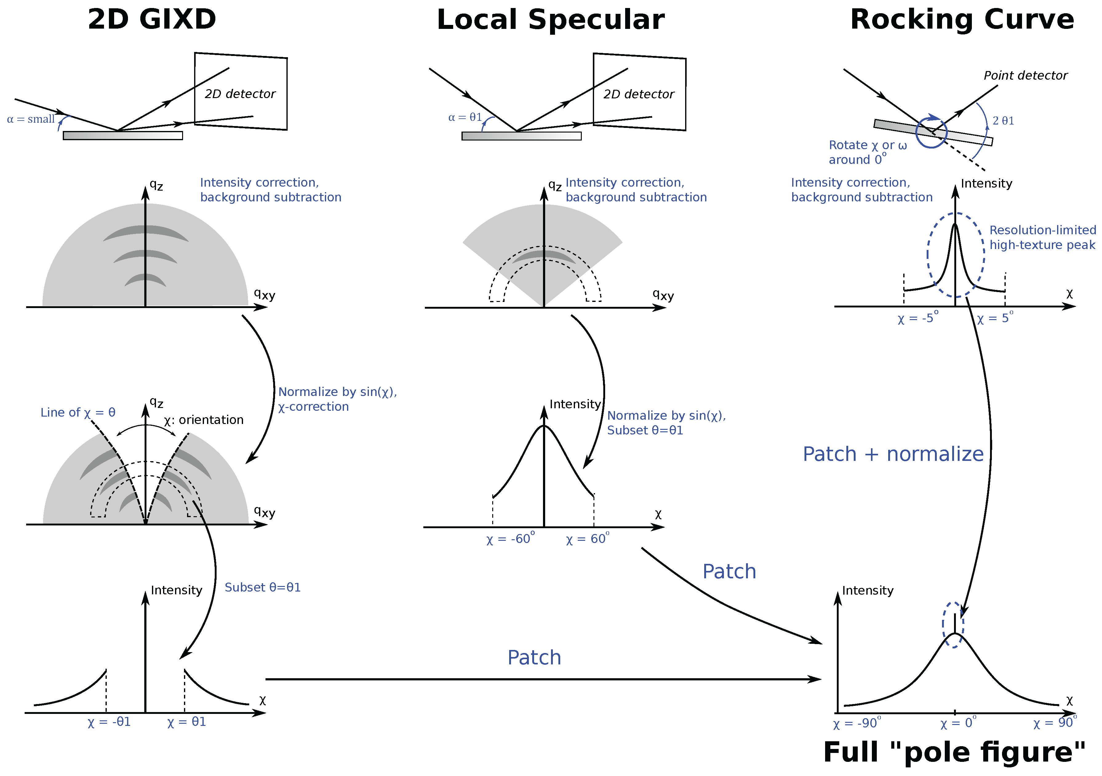
With the proper normalizations, this rich data may offer much insight into the sample. For example, one may compare relative degree of crystallinity, texture, and crystallite size estimation of different samples. References [3,9,44] introduce one such technique that is now commonly used in quantitative texture and degree of crystallinity comparison of polymeric thin films. The technique involves merging of data collected from three synchrotron measurements, and, despite it being developed for electronic polymeric ultra-thin films, is applicable to any uniaxially-textured organic thin films. The essence of the experiment goes as follows: assume that the sample has a uniaxial texture along the sample norm (Figure 1b and Figure 3) and has a known XRD signal at . Then, a radial slice of the 2D GIXD data at constant will uniquely describe the texture of the sample—essentially a pole-figure—and can be used to compare the degree of texture among samples. Relative degree of crystallinity of the samples can be obtained from the area under the curve and can also be compared. The complexity in the technique goes into the details on how to get a complete data set, background subtraction, and normalization, which we shall briefly discuss with the help of Figure 7.
The first data collection, 2D GIXD at slightly above the polymer critical angle, makes up most of the data. This data alone is incomplete because of the forbidden Bragg reflection, causing a “hole” in the data (Section 4.4). Consequently, the first correction is to transform the detector radial angle in the 2D data properly into the actual sample axis . To fill in the hole in GIXD measurements, a specular 2D XRD data is taken at corresponding to the of interest. This second measurement, called the “local specular measurement”, is valid from , except very near . The last measurement, a rocking curve with a high-resolution point detector, is done by setting to the relevant and varying (in this case, equivalent to due to the sample’s uniaxial texture along the sample norm, Figure 3) between and . This measurement is aimed to fill in the small patch near . In References [3,9,44], it has two additional purposes: (1) to investigate the possible presence of resolution-limited super-texture due to vertical spatial confinement of the film, and (2) intensity normalization. The latter is important especially in Reference [3] because the experiment involved various film thicknesses and the authors varied the data integration time for the first two measurements to achieve a good signal-to-noise ratio. The authors then used the normalized photon counts from the last data collection to normalize intensity data in the pole figures that allow for sample-to-sample comparison.
Each individual data must first be background subtracted, 2D data sliced at constant , patched together, and then normalized. Furthermore, data slices from 2D GIXD need to be corrected by a factor of to account for geometrical factors prior to patching [3,9,44]. Patching slices from 2D GIXD and local specular data can be done as follows: first, identify a range in where the data overlap. The two intensity pieces of data should be proportional to each other, the coefficient of which can be obtained from a linear fit of the data from the overlapping region. Therefore, after background subtraction, scaling one of the data sets by (and adding the small constant from) the fit result will ensure a smooth patching. Patching the rocking curve data is done similarly; however, this time, the peak intensity is set to equal the normalized intensity of the rocking curve data.
From this pole figure, one may readily compare the relative degree of crystallinity of the samples as obtained from the area under the intensity curve, and the degree of uni-axial texture of the sample, which is inversely related to the peak width in . These data can then be correlated to, for example, the film’s anisotropic conductivity [8,9,44]. Alternatively, when the samples consist of films of the same material but different thicknesses, this kind of data may offer a significant semi-qualitative insight into the kinetics of film deposition [3,17].
GIXD with a 2D-detector, however, is not a solve-all technique. Measurements such as Warren–Averbach analysis require both much higher resolution than what is offered by 2D-detectors and a long scan range that spans multiple diffraction orders. In this case, the approriate approach is to start with a preliminary measurement using a 2D-detector to locate the peaks, followed by a high-resolution scan [10].
5. Conclusions
We have briefly reviewed contemporary XRD techniques suitable for polymeric thin films and covered the theoretical model behind them. XRD can be utilized to identify chemical composition, quantify degree of crystallinity, texture, crystallite size, and relative degree of disorder in a sample. There are various XRD measurement geometries that are suitable for polymeric thin film samples, but none is a silver bullet for every problem statement. Bragg–Brentano is the most suitable for peak analysis and the simplest to analyze, but is not optimized for thin-film geometry. GIXD and 2D GIXD are much more suitable for polymeric thin films because of higher irradiation volume and lower background, but involve many correction factors, the crystallite orientation being sampled is different for each Bragg angle, and not every crystallite orientation can be sampled. On the other hand, pole figure is a special technique used to map all crystallite orientations for a given Bragg angle. A careful investigator should choose the most suitable geometry by the type of analysis that they have. Furthermore, if possible, X-ray wavelength and scanned axes should be chosen to optimize measurement precision. A combination of a 2D GIXD technique followed by high-resolution scans using a point detector is often necessary to achieve high-quality data while not missing any peaks, and having a reasonable data collection time. For ultra thin films less than ∼ m, the use of synchrotron radiation is most probably necessary.
Acknowledgments
This work did not receive any specific grant from funding agencies in the public, commercial, or not-for-profit sectors. The author thanks Joseph J. Berry, Philip A. Parilla, and Michael F. Toney for their guidance and in-depth discussions.
Conflicts of Interest
The author declares no conflict of interest.
References
- Xu, Z.; Chen, L.M.; Yang, G.; Huang, C.H.; Hou, J.; Wu, Y.; Li, G.; Hsu, C.S.; Yang, Y. Vertical phase separation in poly(3-hexylthiophene): Fullerene derivative blends and its advantage for inverted structure solar cells. Adv. Funct. Mater. 2009, 19, 1227–1234. [Google Scholar] [CrossRef]
- Campoy-Quiles, M.; Ferenczi, T.; Agostinelli, T.; Etchegoin, P.G.; Kim, Y.; Anthopoulos, T.D.; Stavrinou, P.N.; Bradley, D.D.C.; Nelson, J. Morphology evolution via self-organization and lateral and vertical diffusion in polymer: Fullerene solar cell blends. Nat. Mater. 2008, 7, 158–164. [Google Scholar] [CrossRef] [PubMed]
- Widjonarko, N.E.; Schulz, P.; Parilla, P.A.; Perkins, C.L.; Ndione, P.F.; Sigdel, A.K.; Olson, D.C.; Ginley, D.S.; Kahn, A.; Toney, M.F.; et al. Impact of hole transport layer surface properties on the morphology of a polymer-fullerene bulk heterojunction. Adv. Energy Mater. 2014, 4, 1301879. [Google Scholar] [CrossRef]
- Mauger, S.A.; Chang, L.; Friedrich, S.; Rochester, C.W.; Huang, D.M.; Wang, P.; Moulé, A.J. Self-assembly of selective interfaces in organic photovoltaics. Adv. Funct. Mater. 2013, 23, 1935–1946. [Google Scholar] [CrossRef]
- Ashcroft, N.W.; Mermin, N.D. Solid State Physics, 1st ed.; Brooks/Cole: Belmont, CA, USA, 1976. [Google Scholar]
- Kittel, C. Introduction to Solid State Physics, 7th ed.; John Wiley & Sons: Toronto, ON, Canada, 1996. [Google Scholar]
- Prosa, T.J.; Winokur, M.J.; Moulton, J.; Smith, P.; Heeger, A.J. X-ray structural studies of poly(3-alkylthiophenes): An example of an inverse comb. Macromolecules 1992, 25, 4364–4372. [Google Scholar] [CrossRef]
- Sirringhaus, H.; Brown, P.J.; Friend, R.H.; Nielsen, M.M.; Bechgaard, K.; Langeveld-Voss, B.M.W.; Spiering, A.J.H.; Janssen, R.A.J.; Meijer, E.W.; Herwig, P.; et al. Two-dimensional charge transport in self-organized, high-mobility conjugated polymers. Nature 1999, 401, 685–688. [Google Scholar] [CrossRef]
- Baker, J.L.; Jimison, L.H.; Mannsfeld, S.; Volkman, S.; Yin, S.; Subramanian, V.; Salleo, A.; Alivisatos, A.P.; Toney, M.F.; Science, M.; et al. Quantification of Thin Film Crystallographic Orientation Using X-ray Diffraction with an Area Detector. Langmuir 2010, 26, 9146–9151. [Google Scholar] [CrossRef] [PubMed]
- Rivnay, J.; Noriega, R.; Kline, R.; Salleo, A.; Toney, M. Quantitative analysis of lattice disorder and crystallite size in organic semiconductor thin films. Phys. Rev. B 2011, 84, 1–20. [Google Scholar] [CrossRef]
- Miller, N.C.; Cho, E.; Junk, M.J.N.; Gysel, R.; Risko, C.; Kim, D.; Sweetnam, S.; Miller, C.E.; Richter, L.J.; Kline, R.J.; et al. Use of X-ray diffraction, molecular simulations, and spectroscopy to determine the molecular packing in a polymer-fullerene bimolecular crystal. Adv. Mater. 2012, 24, 6071–6079. [Google Scholar] [CrossRef] [PubMed]
- Rivnay, J.; Mannsfeld, S.C.B.; Miller, C.E.; Salleo, A.; Toney, M.F. Quantitative determination of organic semiconductor microstructure from the molecular to device scale. Chem. Rev. 2012, 112, 5488–5519. [Google Scholar] [CrossRef] [PubMed]
- DeLongchamp, D.; Kline, R.; Herzing, A. Nanoscale structure measurements for polymer-fullerene photovoltaics. Energy Environ. Sci. 2012, 5, 5980–5993. [Google Scholar] [CrossRef]
- Salleo, A.; Kline, R.; DeLongchamp, D.; Chabinyc, M. Microstructural characterization and charge transport in thin films of conjugated polymers. Adv. Mater. 2010, 22, 3812–3838. [Google Scholar] [CrossRef] [PubMed]
- Lindenmeyer, P.; Beumer, H.; Hosemann, R. The origin in thermodynamic stability of paracrystals. Prog. Colloid Polym. Sci. 1978, 64, 232–237. [Google Scholar]
- Jimison, L.H.; Toney, M.F.; McCulloch, I.; Heeney, M.; Salleo, A. Charge-transport anisotropy due to grain boundaries in directionally crystallized thin films of regioregular poly(3-hexylthiophene). Adv. Mater. 2009, 21, 1568–1572. [Google Scholar] [CrossRef]
- Duong, D.T.; Toney, M.F.; Salleo, A. Role of confinement and aggregation in charge transport in semicrystalline polythiophene thin films. Phys. Rev. B 2012, 86, 205205. [Google Scholar] [CrossRef]
- Frenkel, J. On pre-breakdown phenomena in insulators and electronic semi-conductors. Phys. Rev. 1938, 54, 647–648. [Google Scholar] [CrossRef]
- Rose, A. Concepts in Photoconductivity and Allied Problems; Interscience: New York, NY, USA, 1963. [Google Scholar]
- Mort, J. Conductive polymers. Science 1980, 208, 819–825. [Google Scholar] [CrossRef] [PubMed]
- Rivnay, J.; Noriega, R.; Northrup, J.; Kline, R.; Toney, M.; Salleo, A. Structural origin of gap states in semicrystalline polymers and the implications for charge transport. Phys. Rev. B 2011, 83, 1–4. [Google Scholar]
- Hosemann, R.; Bagchi, S.N. The interference theory of ideal paracrystals. Acta Crystallogr. 1952, 5, 612–614. [Google Scholar] [CrossRef]
- Hosemann, R. Small-angle scattering of microparacrystallites (mPC’s). J. Appl. Crystallogr. 1978, 11, 540–541. [Google Scholar] [CrossRef]
- Baltá-Calleja, F.J.; Hosemann, R. The limiting size of natural paracrystals. J. Appl. Crystallogr. 1980, 13, 521–523. [Google Scholar] [CrossRef]
- Hosemann, R.; Vogel, W.; Weick, D. Novel aspects of the real paracrystal. Acta Crystallogr. Sect. A Found. 1981, 37, 85–91. [Google Scholar] [CrossRef]
- Hosemann, R. Solid state physics of microparacrystals. Phys. Scr. 1982, 1982, 142–148. [Google Scholar] [CrossRef]
- Hosemann, R. The α*-law in colloid and polymer science. Prog. Colloid Polym. Sci. 1988, 77, 15–25. [Google Scholar]
- Hindeleh, A.M.; Hosemann, R. Paracrystals representing the physical state of matter. J. Phys. C Solid State Phys. 1988, 21, 4115–4170. [Google Scholar] [CrossRef]
- Warren, B.E.; Averbach, B.L. The separation of cold-work distortion and particle size broadening in X-ray patterns. J. Appl. Phys. 1952, 23, 497. [Google Scholar] [CrossRef]
- Drits, V.A.; Eberl, D.D.; Srodon, J. XRD measurement of mean thickness, thickness distribution and strain for illite and illite-smectite crystallites by the Bertaut-Warren-Averbach technique. Clays Clay Miner. 1998, 46, 38–50. [Google Scholar] [CrossRef]
- Knapp, E.W. Lineshapes of molecular aggregates, exchange narrowing and intersite correlation. Chem. Phys. 1984, 85, 73–82. [Google Scholar] [CrossRef]
- Knoester, J. Nonlinear optical susceptibilities of disordered aggregates: A comparison of schemes to account for intermolecular interactions. Phys. Rev. A 1993, 47, 2083–2098. [Google Scholar] [CrossRef] [PubMed]
- Barford, W. Exciton transfer integrals between polymer chains. J. Chem. Phys. 2007, 126, 134905. [Google Scholar] [CrossRef] [PubMed]
- Spano, F.C. The spectral signatures of frenkel polarons in H-and J-aggregates. Acc. Chem. Res. 2009, 43, 429–439. [Google Scholar] [CrossRef] [PubMed]
- Clark, J.; Chang, J.F.; Spano, F.C.; Friend, R.H.; Silva, C. Determining exciton bandwidth and film microstructure in polythiophene films using linear absorption spectroscopy. Appl. Phys. Lett. 2009, 94, 163306. [Google Scholar] [CrossRef]
- Cullity, B. Elements of X-ray Diffraction, 2nd ed.; Addison-Wesley Longman, Inc.: Reading, MA, USA, 1977. [Google Scholar]
- Warren, B.E. X-ray Diffraction; Dover Pubns: New York, NY, USA, 1990. [Google Scholar]
- Smilgies, D.M. Geometry-independent intensity correction factors for grazing-incidence diffraction. Rev. Sci. Instrum. 2002, 73, 1706. [Google Scholar] [CrossRef]
- Buerger, M.J. The correction of X-ray diffraction intensities for Lorentz and polarization factors. Proc. Natl. Acad. Sci. USA 1940, 26, 637–642. [Google Scholar] [CrossRef] [PubMed]
- Heizmann, J.J.; Vadon, A.; Schlatter, D.; Bessieres, J. Texture analysis of thin films and surface layers by low incidence angle X-ray diffraction. Adv. X-ray Anal. 1989, 32, 285–292. [Google Scholar]
- Toney, M.F.; Brennan, S. Observation of the effect of refraction on X-rays diffracted in a grazing-incidence asymmetric Bragg geometry. Phys. Rev. B 1989, 39, 7963–7966. [Google Scholar] [CrossRef]
- He, B.B.; Preckwinkel, U.; Smith, K.L. Fundamentals of two-dimensional X-ray diffraction (XRD2). Adv. X-ray Anal. 2000, 43, 273–280. [Google Scholar]
- Mannsfeld, S.C.B.; Virkar, A.; Reese, C.; Toney, M.F.; Bao, Z. Supplementary info for precise structure of pentacene monolayers on amorphous silicon oxide and relation to charge transport. Adv. Mater. 2009, 21, 2294–2298. [Google Scholar] [CrossRef]
- Jimison, L.H.; Himmelberger, S.; Duong, D.T.; Rivnay, J.; Toney, M.F.; Salleo, A. Vertical confinement and interface effects on the microstructure and charge transport of P3HT thin films. J. Polym. Sci. B Polym. Phys. 2013, 51, 611–620. [Google Scholar] [CrossRef]
Figure 1.
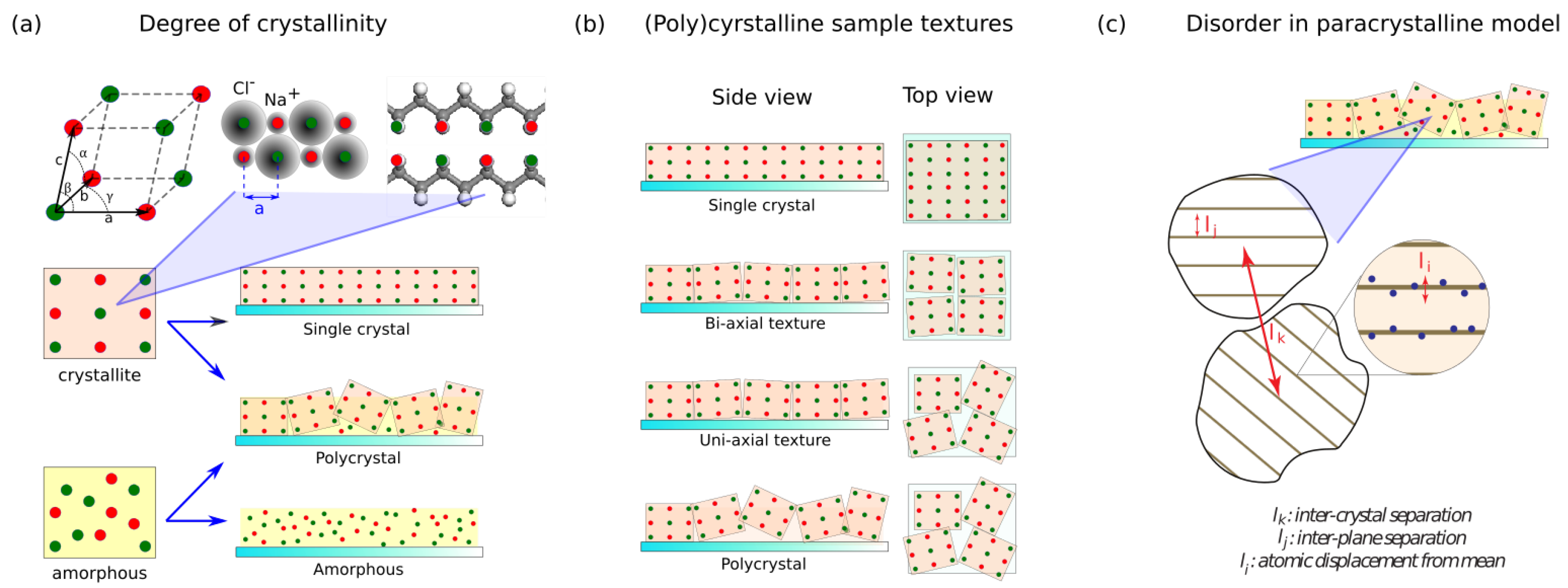
Structural order and disorder. (a) Illustration of a periodic atomic placement in a crystallite and lack of thereof in an amorphous material. Note that the reflecting centers can be atoms in an inorganic compound or part of an organic compound. A polycrystalline sample comprises of a mixture of both crystallites and amorphous parts. The more crystallites in a sample, the higher its degree of crystallinity. (b) Illustration of sample texture. Texture is the statistical description of crystallite orientations in a sample. A bi-axial texture means crystallites in the sample are aligned on two axes (by symmetry, this necessarily means that they are aligned on the third axis too). By definition, a single crystal sample is bi-axially textured. In contrast, crystallites in a uniaxially textured sample are aligned only on one axis. Lastly, in a sample with no texture, crystallites are oriented randomly in three dimensions. (c) Illustration of disorder in the paracrystal model. , , and are the possible atomic displacements from their ideal position in a crystal lattice. Out of these three, only and are included in Hosemann’s paracrystal theory and therefore quantifiable through XRD [15].
Figure 1.
Structural order and disorder. (a) Illustration of a periodic atomic placement in a crystallite and lack of thereof in an amorphous material. Note that the reflecting centers can be atoms in an inorganic compound or part of an organic compound. A polycrystalline sample comprises of a mixture of both crystallites and amorphous parts. The more crystallites in a sample, the higher its degree of crystallinity. (b) Illustration of sample texture. Texture is the statistical description of crystallite orientations in a sample. A bi-axial texture means crystallites in the sample are aligned on two axes (by symmetry, this necessarily means that they are aligned on the third axis too). By definition, a single crystal sample is bi-axially textured. In contrast, crystallites in a uniaxially textured sample are aligned only on one axis. Lastly, in a sample with no texture, crystallites are oriented randomly in three dimensions. (c) Illustration of disorder in the paracrystal model. , , and are the possible atomic displacements from their ideal position in a crystal lattice. Out of these three, only and are included in Hosemann’s paracrystal theory and therefore quantifiable through XRD [15].

Figure 2.
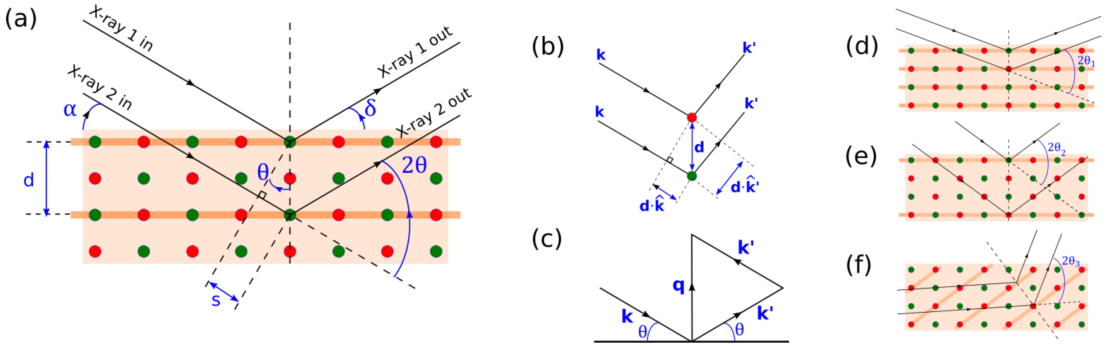
(a) Condition for constructive interference in XRD. Red and blue circles represents scattering centers for X-rays. is X-ray incidence angle, is X-ray exit angle. d is the separation between Bragg (reflecting) planes, and s is half the path difference between two rays. is the Bragg angle. Bragg planes are indicated by thick orange lines. (b) Generalized vectorial description of subfigure (a). (c) Vectorial description of the condition governing constructive interference; Changing leads to a different set of Bragg planes with different d (d,e). Changing an X-ray wavelength will also change in a similar way. On the other hand, changing incidence/exit angle allows us to sample Bragg planes that are not parallel to the sample surface (f).
Figure 2.
(a) Condition for constructive interference in XRD. Red and blue circles represents scattering centers for X-rays. is X-ray incidence angle, is X-ray exit angle. d is the separation between Bragg (reflecting) planes, and s is half the path difference between two rays. is the Bragg angle. Bragg planes are indicated by thick orange lines. (b) Generalized vectorial description of subfigure (a). (c) Vectorial description of the condition governing constructive interference; Changing leads to a different set of Bragg planes with different d (d,e). Changing an X-ray wavelength will also change in a similar way. On the other hand, changing incidence/exit angle allows us to sample Bragg planes that are not parallel to the sample surface (f).

Figure 3.
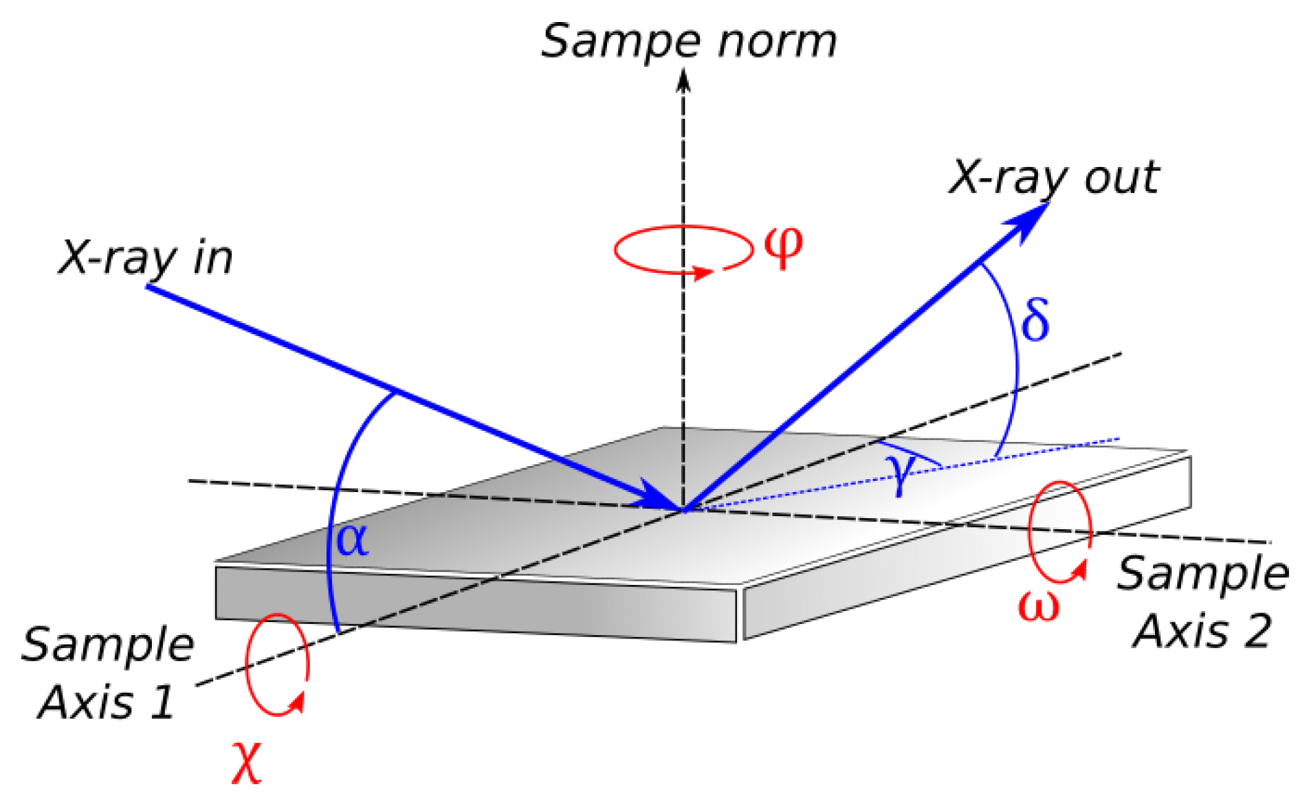
Axes and angles in an XRD measurement. Let Sample axis 1 be the projection of the incoming X-ray on the sample surface, and Sample axis 2 be the axis perpendicular to sample axis 1 and the sample norm. X-ray incident angle () and in-plane exit angle () are measured from sample axis 1. X-ray out-of-plane exit angle () is measured from the sample surface. Sample rotation around its norm () is typically measured from the direction of incident X-ray along sample axis 1. Sample rotation around the axis perpendicular to its norm () is measured from sample norm. Note that . Please also note that rotation around sample axis 2 is measured from the sample norm and is known as .
Figure 3.
Axes and angles in an XRD measurement. Let Sample axis 1 be the projection of the incoming X-ray on the sample surface, and Sample axis 2 be the axis perpendicular to sample axis 1 and the sample norm. X-ray incident angle () and in-plane exit angle () are measured from sample axis 1. X-ray out-of-plane exit angle () is measured from the sample surface. Sample rotation around its norm () is typically measured from the direction of incident X-ray along sample axis 1. Sample rotation around the axis perpendicular to its norm () is measured from sample norm. Note that . Please also note that rotation around sample axis 2 is measured from the sample norm and is known as .

Figure 4.
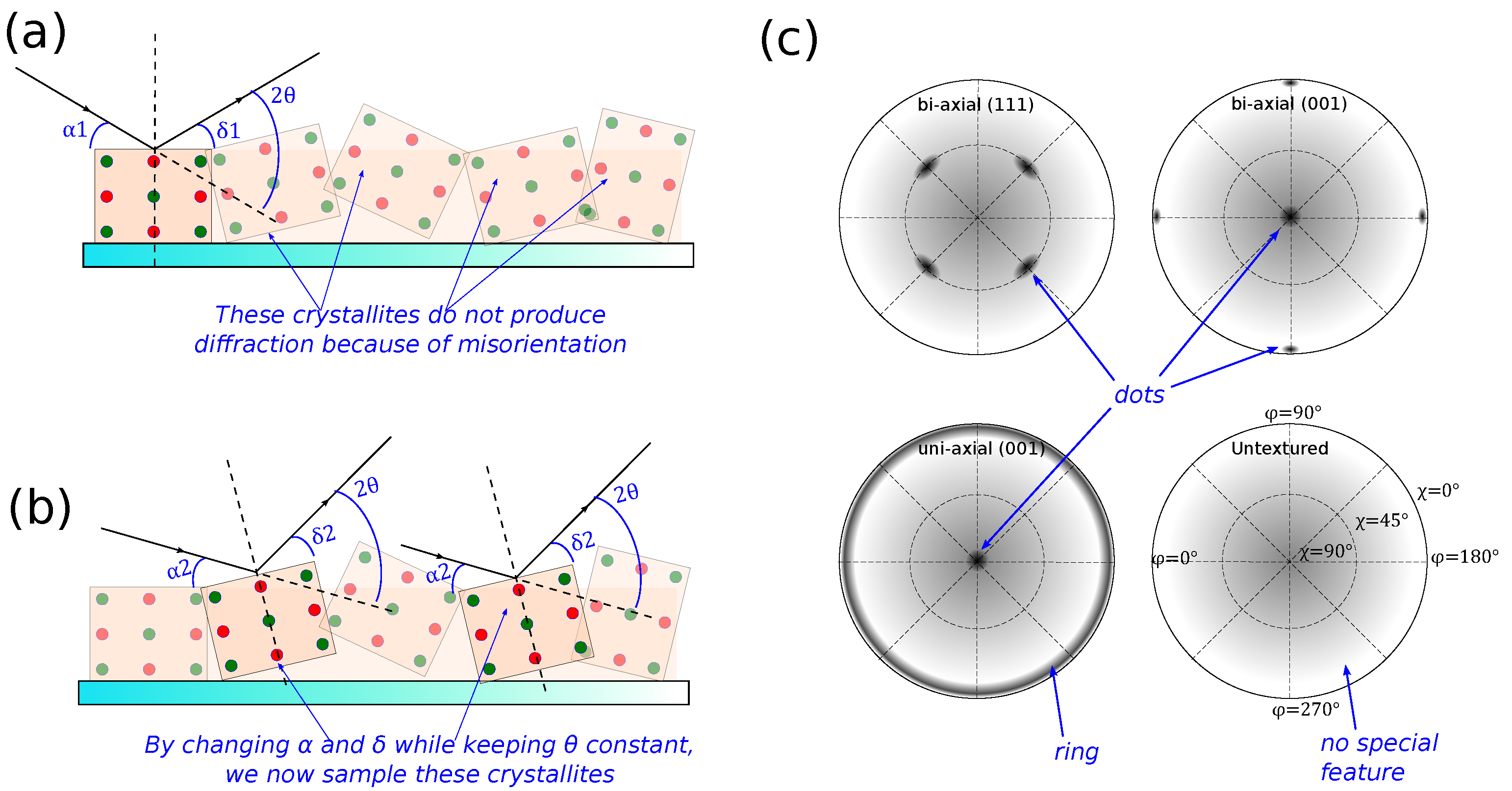
Illustration of how a pole figure works. (a) for a given set of , , and , only some crystallites in the sample produces diffraction. Other crystallites do not satisfy either Bragg condition, i.e., are misoriented. (b) By keeping constant but changing , and , one may sample other misoriented crystallites with the same Bragg condition. (c) Examples of how pole-figure data would look for the textures given on Figure 1b. The angles and are as defined in Figure 3. Because of the thin-film nature of the sample, expect some background from the sample substrate. For example, an amorphous substrate (e.g., glass), will manifest in a low background that is strongest in the center () and fading towards the edge (). Similarly, polycrystalline samples with low texture exhibit no special features, while those with high texture will have dots. As such, a sample with uni-axial texture will have combinations of dots and rings.
Figure 4.
Illustration of how a pole figure works. (a) for a given set of , , and , only some crystallites in the sample produces diffraction. Other crystallites do not satisfy either Bragg condition, i.e., are misoriented. (b) By keeping constant but changing , and , one may sample other misoriented crystallites with the same Bragg condition. (c) Examples of how pole-figure data would look for the textures given on Figure 1b. The angles and are as defined in Figure 3. Because of the thin-film nature of the sample, expect some background from the sample substrate. For example, an amorphous substrate (e.g., glass), will manifest in a low background that is strongest in the center () and fading towards the edge (). Similarly, polycrystalline samples with low texture exhibit no special features, while those with high texture will have dots. As such, a sample with uni-axial texture will have combinations of dots and rings.

Figure 5.
Illustration of GIXD (a–b) and the “hole” in GIXD data (c–d). (a) Illustration of XRD done at a high incident angle on a thin film. Note that the beam spot is small and that the XRD may penetrate through the thin sample. (b) The same measurement but done at low incident angle, causing the beam spot to widen, hence reducing X-ray flux on the sample and reducing X-ray damage. In this configuration, X-rays will also be less likely to penetrate through the sample, resulting in higher signal and reduced background, making this configuration very suitable for thin-film samples. (c) The extreme crystallite orientations that can be measured at a fixed incoming angle. These two extremes are defined by outgoing beam parallel and perpendicular to sample surface. (d) The cone subtended by , within which crystallite orientations will not satisfy Bragg condition, producing a hole in the data.

Figure 6.
Illustration of XRD with a 2D detector, showing the measurement geometry and illustration of image data from samples with different textures. A 2D detector enables the user to take a “picture” of the diffraction pattern, effectively providing data that are usually obtained from multiple XRD scans using point and 1D detectors at the expense of data resolution. A radial slice of the 2D data provides the usual information on . On the other hand, the angular slice of the data provides insight on the film texture. For example, data from a polycyrstalline film appears as rings, a single crystal as dots, and an amorphous material as having no special feature. Data from a sample with texture somewhere in-between these extremes will appear as partial rings. Additionally, macro strains on the sample result in shifted dots or stretched rings. Lastly, in grazing incidence geometry, the region close to the origin of the detector is usually covered by beam stops to prevent damage from direct X-ray radiation, leaving a small hole in the data that is not illustrated here.

Figure 7.
Illustration of the steps to create a full pole-figure in for uniaxially-textured thin-film samples. The final data is patched from three different measurements: a 2D GIXD, a “local specular”, and a rocking curve. is the angle corresponding to the of interest. First, each data set is properly intensity-corrected and background subtracted. Note that data from rocking curve may not contain the peak from highly-textured part of the sample as described in the figure. Data from 2D GIXD is then transformed to correct and its intensity is normalized by to correct for geometrical factor. Next, all 2D data are then subset around . Lastly, all three data sets are patched together.

© 2016 by the author; licensee MDPI, Basel, Switzerland. This article is an open access article distributed under the terms and conditions of the Creative Commons Attribution (CC-BY) license (http://creativecommons.org/licenses/by/4.0/).
Share and Cite
MDPI and ACS Style
Widjonarko, N.E. Introduction to Advanced X-ray Diffraction Techniques for Polymeric Thin Films. Coatings 2016, 6, 54. https://doi.org/10.3390/coatings6040054
AMA Style
Widjonarko NE. Introduction to Advanced X-ray Diffraction Techniques for Polymeric Thin Films. Coatings. 2016; 6(4):54. https://doi.org/10.3390/coatings6040054
Chicago/Turabian StyleWidjonarko, Nicodemus Edwin. 2016. "Introduction to Advanced X-ray Diffraction Techniques for Polymeric Thin Films" Coatings 6, no. 4: 54. https://doi.org/10.3390/coatings6040054
Note that from the first issue of 2016, this journal uses article numbers instead of page numbers. See further details here.