Creating a Consistent Multi-Decadal Oceanic TRMM-GPM Brightness Temperature Record with Estimated Calibration Uncertainty


1
Department of Earth and Environmental Sciences, Vanderbilt University, Nashville, TN 37240, USA
2
Department of Electrical and Computer Engineering, University of Central Florida, Orlando, FL 32816, USA
*
Author to whom correspondence should be addressed.
Climate 2020, 8(2), 31; https://doi.org/10.3390/cli8020031
Submission received: 30 December 2019
/
Revised: 4 February 2020
/
Accepted: 5 February 2020
/
Published: 10 February 2020
Abstract
:The National Aeronautics and Space Administration’s (NASA) Precipitation Measurement Missions (PMMs) include two earth satellite missions, namely, the Tropical Rainfall Measuring Mission (TRMM, 1997–2015) and the Global Precipitation Measurement (GPM, 2014-present). To generate a consistent multi-decadal brightness temperature (Tb) record that spans the TRMM and GPM eras, it is highly desirable to perform a comprehensive intercalibration of the TRMM Microwave Imager (TMI) and the GPM Microwave Imager (GMI) Tb measurements. Unfortunately, GMI and TMI share a limited common operational period of only 13 months. Fortunately, the WindSat polarimetric radiometer (2003-present) has been shown to be well calibrated and radiometrically stable relative to TMI for a period of over 5 years. Therefore, this paper describes the use of overlapping WindSat Tb measurements as the calibration bridge to achieve a seamless transfer joining the TMI and GMI Tb time series. Also, the development of the Tb measurement uncertainty estimation model is presented, which incorporates all relevant sources of uncertainty. Afterwards, this model was applied to three intercalibration processes: TMI to GMI, TMI to WindSat, and WindSat to GMI, and results are presented that quantify the corresponding Tb channel measurements biases and associated uncertainties associated with the merged TMI-GMI Tb record. This is an important accomplishment because this study can enable improved future Earth Science and global climate change investigations by making a long-term Tb record with estimated uncertainty available.
1. Introduction
The Tropical Rainfall Measuring Mission (TRMM), launched on November 27, 1997, was a joint Earth Science satellite mission between the National Aeronautics and Space Administration (NASA) and the Japan Aerospace Exploration Agency (JAXA). Originally, TRMM was intended to be a 3 year science mission to study the statistics of rainfall from the tropical and subtropical regions of the Earth [1]; however, the satellite and its instruments performed in an exceptional manner for 17-plus years, thereby providing a legacy of microwave radiometric data for studying global climate change. The follow-on Global Precipitation Measurement (GPM; see the Appendix A for a list of key acronyms and abbreviations used in this paper) mission, launched in February 2014, employs a constellation of cooperative satellites with microwave sensors, to unify and advance precipitation measurements with the scientific objective of improving the understanding of the Earth’s water and energy cycles [2].
Both GPM and TRMM operate in non-sun-synchronous orbits, which results in regular daily near-coincident intersections with all the sun-synchronous polar-orbiting spacecrafts that comprise the GPM constellation. The GPM Microwave Imager (GMI), on board the GPM observatory, has been demonstrated to be a well-calibrated instrument with exceptional stability [3].Therefore, a major role of the GMI is to serve as a brightness temperature (Tb) calibration standard for the other constellation members; and prior to the launch of GPM, the TRMM Microwave Imager (TMI), on board the TRMM satellite, served this purpose. Based on available on-board propellant for orbit maintenance, the GPM spacecraft operational life is estimated to be 10–15 years [3]. Because the radiometric transfer standard has changed to GMI, it is highly desirable to perform microwave radiometric intercalibration between GMI and TMI to join these precipitation measurements to form a multi-decadal climate dataset [4].
The most critical tests of climate model predictions occur using observations of decadal changes in climate forcing, response, and feedback variables. Many of these key climate variables are observed by remotely sensing the global distribution of reflected solar spectral and broadband radiance. One important primary environmental parameter that has been inferred from microwave Tbs is precipitation, including snow and ice [5]. More accurate global precipitation estimates improve the accuracy and effectiveness of climate models and reanalysis, where the large-scale oceanic or atmospheric patterns may be observed [6]. Durman et al. [7] analyzed the ability of a general circulation model and a high-resolution regional climate model in simulating daily precipitation, by reference to observations; while Serreze and Hurst [8], examined the accuracy of mean precipitation forecasts from the National Centers for Environmental Prediction (NCEP) and European Centre for Medium-Range Weather Forecasts (ECMWF) reanalysis models. Further, long-term precipitation data, helps scientists more accurately estimate the rate of water transfer within the Earth’s atmosphere and on the surface. For example, Skofronick-Jackson et al. examined the detailed structure of the monsoon precipitation, as it moves from south to north across India over seasons, using GPM data from 2014 to 2016 [9]. Precipitation also reconciles the different parts of the overall water budget. Measurements of surface water fluxes, cloud/precipitation microphysics and latent heat release in the atmosphere improve Earth system modeling and analysis. TMI and GMI have provided, and will continue to contribute to, Tb products as references for their partner constellation sensors, and direct inputs for the precipitation algorithm (GPROF) producing the Integrated Multi-satellite Retrievals for GPM (IMERG). The high-resolution spatial scale (0.1° × 0.1°) and temporal scale (30 min) of the IMERG product can be used to advance the understanding of global, regional, convective and microphysical precipitation processes, which are fundamental to regulating our climate.
Because precipitation is one of the key-state variables in studies of climate change and hydrology, it is of increasing importance to understand and predict these processes. Thus, the utility of creating a consistent long-term Tb product from which precipitation is derived is a high priority. Therefore, it is significant to bridge the Tb time series of TMI and GMI, from which a multi-decadal (expected 27–32 years) unified Tb record will be formed, especially when its uncertainty budget is also quantified.
TMI and GMI share a 13 month overlap period (March 2014–March 2015), which allows an inter-satellite radiometric calibration between them; however, there remains a concern about the stability of TMI over its 17-plus years lifetime. Fortunately, the Naval Research Laboratory’s WindSat polarimetric radiometer has operated since January 2003 and has been demonstrated to be stable and to provide accurate Sensor Data Records (SDR) [10,11]; but these data have not been incorporated into the GPM constellation yet. Since the WindSat time series spans the measurements of both TMI and GMI, it can be used to mitigate the TMI long-term radiometric calibration stability concern. The TMI, GMI and WindSat are similar conical-scanning radiometers, and the instrument parameters for the common, precipitation measuring, channels are listed in Table 1. Previously, an inter-satellite radiometric calibration analysis of TMI relative to WindSat was performed, which exhibited exceptional long-term radiometric stability between two one-year windows (2005-2006 and 2011) that were separated by five years [12]. Also, the three-way (WindSat, TMI and GMI) intersatellite radiometric comparisons (during the 13 month overlap), were performed to bridge the TRMM and GPM eras and thereby assure a stable radiometric calibration between the diverse constellation member radiometers [13]. This paper presents results that extends the intercalibration of TMI and WindSat to six one-year periods (2005–2006, 2007, 2011,2012, 2013 and 2014) using the legacy product of TMI Tb data (1B11 V8). The new version of TMI Tbs has improvements on several issues over the old V7 including geolocation, emissive antenna correction, hot load correction, multi-scan calibration, and radio frequency interference [14,15,16,17]. With these results, the derived Tb biases after the composite intercalibration (XCAL) offsets can be applied to the TMI 17-plus years legacy Tb product, to create a consistent multi-decadal TRMM-GPM Tb record. We are aware that the general definition of bias in statistics is the difference between the estimated value and the true value of a certain estimator. However, in previous work (e.g., [4,9,18]), the radiometric difference (discussed below in Section 2) between one sensor and another that is well calibrated (also known as the reference standard) has been referred to as calibration bias, or simply bias, which cannot be regarded as the typical interpretation of bias. Consistent with this literature, we will continue using the term bias to describe the radiometric difference between two sensors. To distinguish the calibration bias from the general form of bias, we would like to treat this calibration bias as a kind of measurand.
Moreover, for purposes of assessing climate change and its effects, it is imperative to address the Tb measurement errors and long-term radiometric calibration stability of the TMI/GMI time series. This requires systematic analysis and consistent methods of incorporating Tb uncertainty estimations into its downstream precipitation product that is significant for global climate change assessments. Thus, a generic uncertainty quantification model is developed based on TMI/GMI intercalibration, and then applied to the intercalibration of TMI/WindSat and WindSat/GMI. This process will provide uncertainties for the TMI/GMI Tb time series.
2. CFRSL XCAL Algorithm
A robust inter-satellite calibration algorithm developed by Central Florida Remote Sensing Lab (CFRSL) has been applied to multiple microwave radiometers. It compares two satellite radiometer observations, on a channel basis, for homogeneous earth scenes that are collocated spatially and temporally. In the simplest sense, if the corresponding channels of two radiometers, with identical design, were to make an observation over the earth at the exact same time and space, the difference in their Tbs should reflect the radiometric calibration bias between the instruments. Unfortunately, for radiometers of different designs, the situation is more complicated due to different center frequencies, bandwidths and/or earth incidence angles; thus, normalization between the instruments is required before cross-calibration. Using the CFRSL XCAL algorithm, this normalization utilizes microwave radiative transfer theory to translate the measurement of an instrument to a common basis before comparison. This algorithm involves three procedures to obtain simulated Tbs, namely, gridding, collocation and radiative transfer model simulation. The double difference technique is then applied to the observed and simulated Tbs, to obtain the calibration biases. A block diagram of these procedures is presented in Figure 1, and more details can be found in Biswas et al. [18].
3. The Uncertainty Quantification Model
While the CFRSL XCAL algorithm yields the radiometric bias that can be applied to the TMI 17-plus years legacy Tb product, there is also an uncertainty in this calibration bias, which must be estimated. As discussed above, the bias here is different from the general definition of bias in statistics. In this study it is the radiometric difference between two sensors, and we consider it as a kind of measurand. To estimate the uncertainty associated with this bias, the uncertainty quantification model (presented herein) sorts six major uncertainty sources and uses various methods to quantify individual uncertainties and finally combine them on a channel basis [19]. It should be noted that the uncertainty in calibration bias is different from an error. By definition, error is the difference between the true bias and the estimated bias. The “true,” or most likely, bias may thus be considered as the estimated bias combined with a statement of uncertainty which characterizes the dispersion of possible collected bias. Uncertainty is caused by the interplay of errors which create dispersion around the estimated bias; the smaller the dispersion, the smaller the uncertainty [20]. Therefore, the uncertainty derived herein will be reported to the NASA Precipitation Processing System (PPS), indicating the uncertainty associated with the estimated averaged Tb bias and not the error. The uncertainty of the Tb bias reflects the lack of exact knowledge of the bias due to various possible sources of uncertainty.
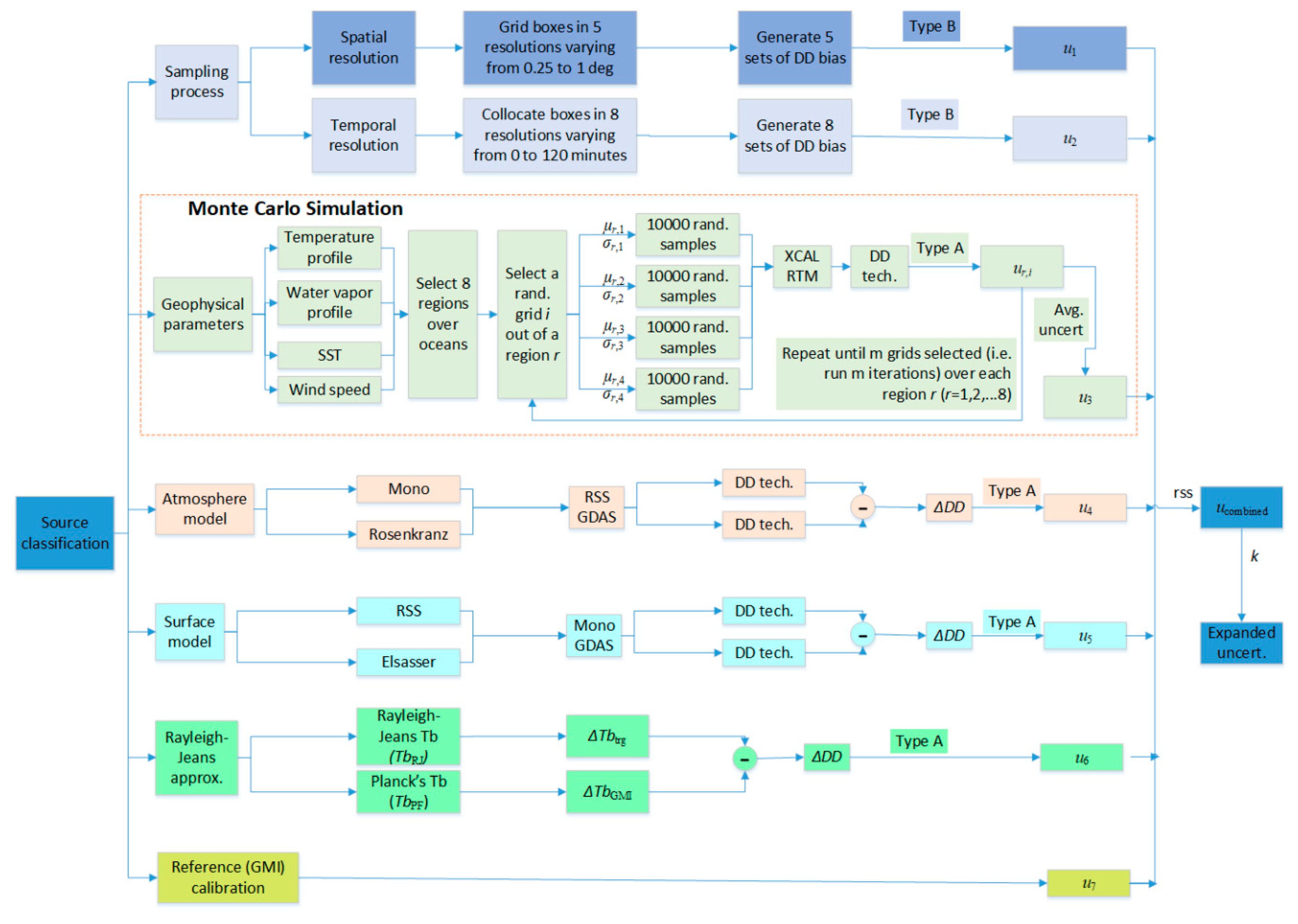
The block diagram of all uncertainty sources and individual uncertainty quantification processes is depicted in Figure 2. In this figure, there are seven parallel paths used to derive estimates of uncertainty for these independent sources. The first two paths concerns sampling process, which (given the sensor footprints of tens of kilometers) results in variability in both time and space. The second path is a Monte Carlo simulation used for quantifying the uncertainty associated with the environmental parameters, which are inputs to radiative transfer models (RTMs). The third and fourth paths are associated with the imperfect physics associated with microwave RTMs for atmosphere absorption and ocean microwave emission. The fifth path is associated with using the Rayleigh approximation to Planck’s blackbody radiation law, and finally the last path is associated with the absolute radiometric calibration of the GMI standard. The Monte Carlo simulation is highlighted by the pink dash-line box within which µ is the bias in the region r of each of the four geophysical parameters: atmospheric temperature profile, water vapor profile, sea surface temperature (SST) and wind speed. The ∆Tbtrg is the Tb deviation of Rayleigh–Jeans approximation from the Planck’s Law for a target (trg) radiometer. More details are provided in the remainder of this section.
3.1. Methods and Data Selection
Calculating the overall uncertainty of the Tb bias requires evaluation of the standard uncertainty of each source that could possibly result in dispersion in the estimated biases relative to the true bias. The accuracy with which the RTM model can predict the true value of Tb, is dependent on the input data, boundary conditions and the model itself. The uncertainty sources investigated here include sampling process (spatial and temporal), geophysical field variation, two atmospheric absorption models, two surface emissivity models, Rayleigh–Jeans approximation to Planck’s Law, and the calibration reference (GMI).
Any method for evaluating uncertainty using statistical analysis of a series of observations is called Type A; whereas, any method for evaluation uncertainty by means other than the statistical analysis for a series of observations is called Type B.
Type A uncertainty estimates are often used in assessing random effects, and the treatment is usually a calculation of the standard deviation (std) expressed as
where vi is one value (bias of one observation) from the population (all biases), µ0 is the population average, and n is the number of repeated experiments (e.g., Monte Carlo simulations that were explained in Section 3.3).
Type B uncertainty estimation is used in systematic effects, and the treatment is expressed by the following equation:
Sample size determination is the act of choosing a sufficient number of observations to include in the uncertainty quantification model development. The sample size is an important feature because samples that are too large may waste time and computer resources, while samples that are too small may lead to inaccurate results. There are two terms that affect the minimum sample size: margin of error and confidence level. In this study, we determined the minimum sample size to estimate the uncertainty of the Tb calibration bias within 0.05 K margin of error and with 99% confidence.
When sample data are collected, and the sample mean is calculated, that sample mean is typically different from the population mean µ. This difference between the sample and population means can be thought of as an error. Then, the margin of error E is the maximum difference between the observed sample mean and the true value of the population mean µ0, and E should meet the following criterion:
where is known as the critical value, the positive z value is the vertical boundary for the area of the probability density function in the right tail of the standard normal distribution, σ0 is the population std and n is the sample size. A 99% confidence then yields α = 0.01 and = 2.576.
Therefore, the n value should meet the following expression:
For illustration purposes, TMI/GMI intercalibration is used to demonstrate the uncertainty quantification process. The largest std of TMI/GMI biases lies in 37 GHz H-pol (0.677 K). Therefore, the minimum sample size derived using Equation (4) is 1217, which should be satisfied throughout the uncertainty quantification model development process. It should be noted that because the minimum sample size is proportional to the std squared, it varies depending on which instrument is intercalibrated to. Other factors, such as confidence level, also contribute to changes in the minimum sample size.
3.2. Uncertainty in the Sampling Process
The commonly used spatial resolution in the CFRSL XCAL algorithm is 1° latitude/longitude, and the temporal resolution is ±60 minutes. The Tb biases change slightly when different spatial or temporal resolutions are used; therefore, it is necessary to estimate the uncertainty of Tb biases caused by resolution variations.
To evaluate this, the CFRSL XCAL algorithm was performed iteratively with different spatial and temporal resolutions, and the standard uncertainty of the sampling process was then calculated based upon the multiple sets of calibration biases. Specifically, eight cases of different temporal resolutions were studied in a time window of 15 min. Therefore, Case 1 was the XCAL of TMI and GMI when their observation time difference was 0–15 min, and the next one was 15–30 min, and so on. The five cases of spatial resolutions with different latitude/longitude box sizes were 1° × 1°, 0.75° × 0.75°, 0.5° × 0.5°, 0.375° × 0.375° and 0.25° × 0.25°, respectively. The highest spatial resolution was equivalent to the GMI instantaneous field of view (IFOV) at 10 GHz (19 ×32 km). Eight sets of mean values and std values of Tb biases were then obtained for temporal sampling variations, and five sets for spatial sampling variations. Using the treatment of the Type B method (Equation (2)), the spatial and temporal standard uncertainties per channel were calculated and listed in Table 2, where the largest value is only 0.018 K in 37 GHz H-pol channel. Given such small values of uncertainties and the considerably large computation resources consumed, we concluded that the impact of resolution variation is insignificant and can be ignored in future uncertainty quantification applications.
3.3. Uncertainty in Geophysical Parameters
Modeling microwave brightness temperature requires knowledge of geophysical parameters such as SST, wind speed, and atmospheric profiles of air temperature and pressure, water vapor and cloud liquid water. These geophysical parameters are used as inputs to the RTM model to calculate theoretical Tbs for given radiometer channels. The primary geophysical parameters are obtained from the NOAA Global Data Assimilation System (GDAS) that uses the NCEP Global Forecast System (GFS) model (NCEP 2000) to provide outputs at 00:00, 06:00, 12:00, and 18:00 Universal Coordinated Time (UTC), on a 1° x 1° latitude/longitude grid [21]. Given that a numerical weather prediction (NWP) model only provides estimates of the true environmental conditions, it is inevitable that the uncertainties of these parameters are propagated to the output theoretical Tbs through the RTM model and then further to the derived Tb biases.
Monte Carlo simulation is an effective technique for evaluating uncertainties where a theoretical approach would be difficult or inconclusive. Because the relationship between RTM inputs (geophysical parameters) and outputs (theoretical Tbs) is rather complex, we used this technique to quantify the uncertainty of the Tb biases propagated from the inherent uncertainty of geophysical parameters.
The Monte Carlo simulation used algorithmically generated pseudo-random numbers, which were forced to follow a prescribed probability distribution. For a normal distribution, the spread of random numbers was predetermined by its specified mean and its std. For each input, the Monte Carlo simulation generated a numeric value drawn at random from its respective probability density function. Numeric values derived in this manner were produced for all inputs to the known functional relationship, which were then used to produce a single numeric value as output. The process was repeated a sufficiently large number of trials to produce a set of simulated results as outputs. The mean and std of these output results were then respective estimates of the measurand and its standard uncertainty. As these input parameters were randomly selected from the predefined probability distributions associated with each of the input variables, the overall process may be considered as a procedure for the propagation of distributions.
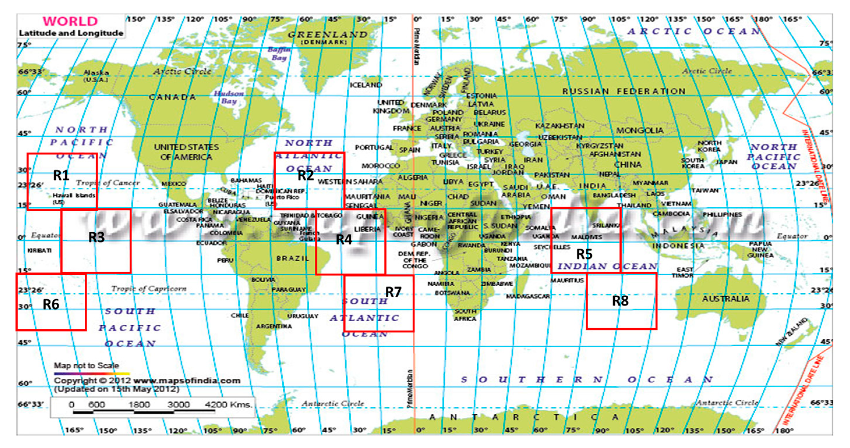
In order to investigate the uncertainty variation of the geophysical parameters associated with geophysical location, eight different oceanic regions were selected within latitudes [45° S, 45° N] and longitudes [180° W, 180° E] (Figure 3). The atmospheric parameters fed into the Monte Carlo simulation included atmospheric temperature profiles and water vapor profiles stored in 21 pressure levels in GDAS, and the surface parameters consisted of SST and wind speed. Based on the mean bias and root mean square (rms) of these parameters for five geographic regions documented by Smith et al in their Table 2 [22], we have extended the analysis to the eight regions shown in Figure 3, by mapping additional three regions out of its original five ones. The bias and rms values of these geophysical parameters over the eight regions are listed in Table 3. In each iteration of the Monte Carlo simulation, a random sample (grid) is selected and 10,000 sets of Gaussian distributed noises with predetermined mean and rms were randomly generated and correspondingly added to the four environmental parameters. These perturbed geophysical fields were then used as inputs to the RTM to simulate theoretical Tbs for the subsequent calibration biases. This Monte Carlo simulation was run for a sufficiently large number of iterations that was greater than the minimum sample size (1300 iterations in this case).
For a single Monte Carlo simulation process, the calibration biases followed a near-Gaussian distribution, which was consistent with the perturbed geophysical parameters’ distributions. Further, the single standard uncertainty was obtained by calculating the std of the calibration biases (Type A treatment). With 1300 iterations of Monte Carlo simulation over each region, the averaged std of the calibration bias derived in this manner was then treated as the standard uncertainty caused by imperfect understanding of the true geophysical parameters.
Next, a total of 10,400 iterations were performed by combining the eight regions, and the averaged regional uncertainties and the average total uncertainty of each channel were calculated (Figure 4). The regional uncertainties were very small for all the channels except the 19 GHz channels that ranged between 0.2 and 1 K, which were proportional to the rms values of water vapor in Table 3.
3.4. Uncertainty in the Rayleigh–Jeans Approximation
The basic quantity collected by a satellite microwave radiometer antenna is the power of non-polarized blackbody electromagnetic radiation at the top of the atmosphere given by Planck’s Law:
where If is the spectral brightness intensity that a blackbody radiates uniformly in all directions with unit Wm−2sr−1Hz−1, h is Planck’s constant (6.63 × 10⁻³⁴ J ∙ s), f is frequency (Hz), k is Boltzmann’s constant (1.38 × 10⁻²³ J∙K−1), T is the blackbody’s absolute temperature (K), and c is the speed of light in vacuum (~3 × 10⁸ m∙s−1).
In the microwave region, it is customary to use the Rayleigh–Jeans approximation (rather than Planck’s Law) because it is mathematically simpler and because of its fractional deviation from Planck’s exact expression is less than 1% if f/T < 3.9 × 10⁸ Hz∙K−1 [23]. Nevertheless, with the uncertainty quantification model, the uncertainty due to this approximation was estimated by using Planck’s Law and Rayleigh–Jeans approximation individually, and then taking the std of their differences. The mathematical expressions were as follows:
where u is the standard uncertainty, TbRJ is the observed Tb from TMI or GMI (the Rayleigh–Jeans approximation), and TbPF is the Planck brightness temperature expressed as follows:
where the Rayleigh–Jeans approximation is the truncation of the right side of Equation (9) at 0th order, which means TbRJ = T.
For each instrument and each sample, the difference between the full Planck’s Law and Rayleigh–Jeans approximation asymptotically approaches , which is extremely small (of order 10−5). Over the full range of TMI frequencies, the Rayleigh–Jeans approximation for intercalibrating microwave radiometers is excellent; therefore, this uncertainty source will be removed from the uncertainty quantification model in the future applications.
3.5. Uncertainty in Different RTMs
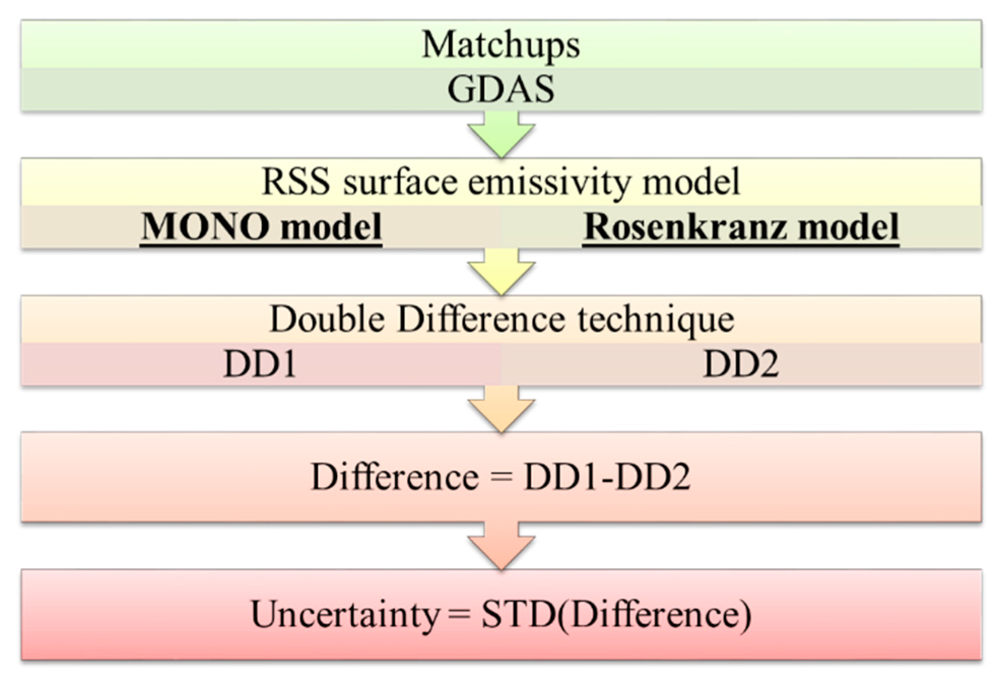
The original NASA XCAL RTM that was used for more than a decade, comprised the Rosenkranz atmospheric absorption model [24,25,26] and the Elsaesser ocean surface emissivity model [27]. Recently this was replaced by the MonoRTM (Mono) [28] atmospheric absorption model and the Remote Sensing System (RSS) ocean surface emissivity model [29]. Thus, the old and new models were used to estimate the uncertainties associated with the RTM physics.
The method used to quantify the RTM uncertainty is shown in Figure 5. The intercalibration of TMI/GMI was implemented twice by keeping all input parameters fixed and changing the atmospheric absorption models (Rosenkranz or Mono). The corresponding calibration biases were calculated and the std of their differences was treated as the uncertainty due to the divergence in atmospheric absorption models, and the derived uncertainties were listed in the first row of Table 4. A similar process was subsequently performed to assess the uncertainty from different surface emissivity models (Elsaesser and RSS) and the results are summarized in the second row of Table 4.
3.6. Uncertainty Combination
Since the uncertainties discussed above originated from different sources, they were considered as independent random uncertainties, which were added in quadrature (AiQ), to calculate the total (combined) standard uncertainty of the estimated calibration bias per channel given as:
where i is the channel number and k is the number of uncertainty sources. Note that, the combined standard uncertainty contains terms whose components are derived from Type A and/or Type B evaluations without discrimination between types. With the standard uncertainties from six independent sources investigated in Table 5, the AiQ uncertainties are calculated and listed in the last row of this table.
The use of GMI as a transfer standard demands its calibration stability and calibration uncertainty to be considered. The design of GMI was predicated on eliminating potential calibration issues, and it has been demonstrated that GMI is a well-designed instrument, with a well-understood calibration uncertainty reported by Draper et al [3]. Now that the GMI calibration uncertainty has been obtained, the overall standard uncertainties were calculated by combining all the seven independent uncertainties (Table 6).
By comparing the AiQ values in Table 5 and the combined standard uncertainty in Table 6, it is noted that the uncertainty is dominated by the GMI calibration uncertainty in all the channels except 19V and 19H, which indicates the importance of using a stable and reliable reference radiometric transfer standard like GMI. It is also recognized that the largest uncertainties in 19 GHz channel probably result from the inadequate knowledge of water vapor in the NWP models and the imperfect radiative transfer modeling of the water vapor resonance near 22.22 GHz. Moreover, because the uncertainties associated with sampling variation and the Rayleigh–Jeans approximation are negligible, they can be omitted from the uncertainty quantification model implementation when computation resources such as time and computer CPU are limited.
4. Intercalibration of TMI/WindSat and WindSat/GMI
The radiometric intercalibration of TMI relative to GMI was performed directly for 13 months, from March 2014 through March 2015. Outside of this time interval, WindSat served as the calibration bridge to provide additional intercalibration for creating a consistent multi-decadal oceanic brightness temperature record. Therefore, it is important to assess the uncertainty as well as the Tb bias for TMI/WindSat and WindSat/GMI intercalibration. WindSat has been in operation since its launch in 2003, and the period that both TMI and WindSat data were available was more than 12 years. In this paper, Tb measurements of TMI and WindSat for six periods of one-year duration, spanning in total more than 8 years (July 2005 to December 2014), were analyzed regarding their calibration biases/uncertainties and long-term consistency.
4.1. Tb Bias
The CFRSL XCAL algorithm was first applied to TMI/GMI to derive the Tb biases listed in Table 7. Next, TMI was intercalibrated relative to WindSat for 6 periods of one-year duration, spanning in total more than 8 years (July 2005 to December 2014). During this time span, the average biases of TMI/WindSat (Table 7) are exceptionally consistent (< 0.1 K) for all channels except for the water vapor channels at 19 GHz and 23 GHz. For these channels, it is noted that the first two years are similar, but a step function change (maximum ~ 0.2 K) occurred at the third year, and this was stable for years 3–6. It is suspected that this is the result of changes in the GDAS NWP model that occurred during this period. Finally, WindSat/GMI intercalibration was performed and the corresponding Tb biases are also given in Table 7.
Next, the calibration biases of TMI/WindSat were stratified into month of the year for the six one-year time series. This comparison is important because the seasonal variation of environmental parameters will result in changes in the monthly-averaged scene brightness temperature; but the radiometric calibration biases are expected to be constant (i.e., independent from scene brightness). Excluding the 19 and 23 GHz channels, results shown in Figure 6 demonstrate a very weak seasonal pattern with peak to peak variations being < 0.1 K. On the other hand, for the water vapor sensitive channels, a peak-to-peak 0.5 K variability occurs at 19 GHz and 23 GHz. Further, it is noted that the first two years are similar, but a step function change (maximum ~ 0.2 K) occurs in the third year.
4.2. Uncertainty
The uncertainty quantification model provided the uncertainties associated with the Tb biases of TMI/GMI, TMI/WindSat and WindSat/GMI intercalibration, and results are given in Table 8. Also, since WindSat provides the calibration bridge between GMI and TMI Tb records, the TMI/WindSat intercalibration uncertainties for the six individual years are shown in Figure 7 for the three major uncertainty sources by radiometer channel. For every channel, the change in uncertainties over the entire time series is negligible (< 0.002 K), which demonstrates the exceptional stability in the long-term intercalibration between TMI and WindSat.
5. Discussion and Conclusions
Earth Science investigations and global climate change studies require consistent long-term precipitation data as input, which increases the need for a long-term unified brightness temperature record. Using the WindSat polarimetric radiometer as a calibration bridge, the results presented in this paper are sufficient for NASA’s GPM project to create a consistent, multi-decadal, intercalibrated TMI/GMI oceanic Tb record. This was accomplished by first performing XCAL between TMI and GMI during their 13 months overlap. Next, XCAL was performed between TMI and WindSat during six one-year periods within the interval of 2005- 2014. Results demonstrate exceptional stability in the calibration biases, from which it can be inferred that both TMI and WindSat are stable. Thus, we have shown that the desired multi-decadal product can be obtained by combining the 17-plus years legacy Tb product with the on-going GMI measurements.
While the CFRSL XCAL algorithm yields the estimated Tb bias (by radiometer channel) that can be applied to this TMI Tb product, there remains a radiometric calibration uncertainty. To estimate this uncertainty, a generic uncertainty quantification model was developed considering all possible sources of uncertainty, namely uncertainties associated with: variability in spatial and temporal resolutions; NWP environmental input parameters; differences between the Rayleigh–Jeans approximation and Planck’s Law; divergence in physics in atmospheric and oceanic surface microwave RTMs; and finally, calibration uncertainty in the radiometric transfer standard, GMI. The presented uncertainty quantification model was subsequently applied to the GMI, TMI and WindSat Tb record. This GPM/TRMM long-term inter-satellite calibrated Tb record with its uncertainty estimate will provide a dataset that can be utilized to make significant scientific advances (especially for climate studies).
Further, this uncertainty quantification model can be applied to the intercalibration of other sensors within the TRMM-GPM constellation. We believe that the process will result in a unified high-sampling-frequency and globally-covered Tb product with associated calibration uncertainties that will allow improved scientific utilization as compared to existing Tb products. While this work has paved the way for quantifying the uncertainty estimates associated with these calibration biases, we recognize that there is room for improvement in the intercalibration for the water vapor sensitive channels. Given the considerable sophistication of the science of water vapor spectroscopy, we doubt that improved RTM physics is likely. Therefore, this suggests that the issue may be associated with the atmospheric water vapor profile input to the RTM. Studies are suggested to use water vapor profiles retrieved from millimeter radiometer sounders’ measurements (rather than numerical weather predictions) to determine the impact on the calibration biases of these problematic channels.
Author Contributions
Conceptualization, R.C. and W.L.J.; methodology, R.C.; software, R.C; supervision, W.L.J; writing—original draft preparation, R.C.; writing—review and editing, W.L.J. All authors have read and agreed to the published version of the manuscript.
Funding
This research was funded by NASA Earth Sciences Division, grant number NNX16AE35G.
Acknowledgments
The authors thank the NASA Precipitation Processing System (PPS) for providing the GPM and TRMM L1B data and the Naval Research Laboratory for providing WindSat data for this research.
Conflicts of Interest
The authors declare no conflict of interest.
Appendix A

Table A1.
List of acronyms.
| AiQ | Added in Quadrature | NCEP | National Centers for Environmental Prediction |
|---|---|---|---|
| CFRSL | Central Florida Remote Sensing Lab | NWP | Numerical Weather Predication |
| CPU | Central Processing Unit | PPS | Precipitation Processing System |
| DD | Double Difference | RMS | Root Mean Squared |
| ECMWF | European Centre for Medium-Range Weather Forecasts | RTM | Radiative Transfer Model |
| GDAS | Global Data Assimilation System | RSS | Remote Sensing System |
| GFS | Global Forecast System | SDR | Sensor Data Records |
| GPROF | Goddard Profiling | SST | Sea Surface Temperature |
| GPM | Global Precipitation Measurement | std | Standard Deviation |
| IFOV | Instantaneous Field of View | Tb | Brightness Temperature |
| IMERG | Integrated Multi-satellitE Retrievals for GPM | TMI | TRMM Microwave Imager |
| JAXA | Japan Aerospace Exploration Agency | TRMM | Tropical Rainfall Measurement Mission |
| Mono | Monochromatic radiative transfer model (MonoRTM) | UTC | Coordinated Universal Time |
| NASA | National Aeronautics and Space Administration | XCAL | Intercalibration |
| NOAA | National Oceanic and Atmospheric Administration |
References
- Simpson, J.; Adler, R.F.; North, G.R. A Proposed Tropical Rainfall Measuring Mission (TRMM) satellite. Bull. Amer. Meteor. Soc. 1988, 69, 278–295. [Google Scholar] [CrossRef] [Green Version]
- Hou, A.Y.; Kakar, R.K.; Neeck, S.; Azarbarzin, A.A.; Kummerow, C.D.; Kojima, M.; Oki, R.; Nakamura, K.; Iguchi, T. The Global Precipitation Measurement Mission. Bull. Amer. Meteor. Soc. 2013, 95, 701–722. [Google Scholar] [CrossRef]
- Draper, D.W.; Newell, D.A.; Wentz, F.J.; Krimchansky, S.; Skofronick-Jackson, G.M. The Global Precipitation Measurement (GPM) Microwave Imager (GMI): Instrument overview and early on-orbit oerformance. IEEE J. Sel. Top. Appl. Earth Obs. Remote Sens. 2015, 8, 3452–3462. [Google Scholar] [CrossRef]
- Berg, W.; Bilanow, S.; Chen, R.; Datta, S.; Draper, D.; Ebrahimi, H.; Farrar, S.; Jones, W.L.; Kroodsma, R.; McKague, D.; et al. Intercalibration of the GPM microwave radiometer constellation. J. Atmos. Oceanic Technol. 2016, 33, 2639–2654. [Google Scholar] [CrossRef]
- Ohring, G.; Wielicki, B.; Spencer, R.; Emery, B.; Datla, R. Satellite instrument calibration for measuring global climate change: Report of a Workshop. Bull. Amer. Meteor. Soc. 2005, 86, 1303–1314. [Google Scholar] [CrossRef]
- Skofronick-Jackson, G.; Kirschbaum, D.; Petersen, W.; Huffman, G.; Kidd, C.; Stocker, E.; Kakar, R. The Global Precipitation Measurement (GPM) mission’s scientific achievements and societal contributions: reviewing four years of advanced rain and snow observations. Q. J. R. Meteorol. Soc. 2018, 144, 27–48. [Google Scholar] [CrossRef] [Green Version]
- Durman, C.F.; Gregory, J.M.; Hassell, D.C.; Jones, R.G.; Murphy, J.M. A comparison of extreme European daily precipitation simulated by a global and a regional climate model for present and future climates. Q. J. R. Meteorol. Soc. 2001, 127, 1005–1015. [Google Scholar] [CrossRef]
- Serreze, M.C.; Hurst, C.M. Representation of mean arctic precipitation from NCEP–NCAR and ERA Reanalyses. J. Climate 2000, 13, 182–201. [Google Scholar] [CrossRef]
- Skofronick-Jackson, G.; Petersen, W.A.; Berg, W.; Kidd, C.; Stocker, E.F.; Kirschbaum, D.B.; Kakar, R.; Braun, S.A.; Huffman, G.J.; Iguchi, T.; et al. The Global Precipitation Measurement (GPM) mission for science and society. Bull. Amer. Meteor. Soc. 2016, 98, 1679–1695. [Google Scholar] [CrossRef]
- Gaiser, P.W.; Germain, K.M.S.; Twarog, E.M.; Poe, G.A.; Purdy, W.; Richardson, D.; Grossman, W.; Jones, W.L.; Spencer, D.; Golba, G.; et al. The WindSat spaceborne polarimetric microwave radiometer: sensor description and early orbit performance. IEEE Trans. Geosci. Remote Sens. 2004, 42, 2347–2361. [Google Scholar] [CrossRef]
- Jones, W.L.; Park, J.D.; Soisuvarn, S.; Hong, L.; Gaiser, P.W.; Germain, K.M.S. Deep-space calibration of the WindSat radiometer. IEEE Trans. Geosci. Remote Sens. 2006, 44, 476–495. [Google Scholar] [CrossRef]
- Chen, R.; Santos-Garcia, A.; Farrar, S.; Jones, W.L. Assessment of the long-term radiometric calibration stability of the TRMM microwave imager and the WindSat satellite radiometers. In Proceedings of the 2014 13th Specialist Meeting on Microwave Radiometry and Remote Sensing of the Environment (MicroRad), Pasadena, CA, USA, 24–27 March 2014; pp. 187–191. [Google Scholar]
- Chen, R.; Ebrahimi, H.; Jones, W.L. Creating a multidecadal ocean microwave brightness dataset: three-way intersatellite radiometric calibration among GMI, TMI, and WindSat. IEEE J. Sel. Top. Appl. Earth Obs. Remote Sens. 2017, 10, 2623–2630. [Google Scholar] [CrossRef]
- Stocker, E.F.; Alquaied, F.; Bilanow, S.; Ji, Y.; Jones, L. TRMM Version 8 reprocessing improvements and incorporation into the GPM data suite. J. Atmos. Oceanic Technol. 2018, 35, 1181–1199. [Google Scholar] [CrossRef]
- Alquaied, F.; Chen, R.; Jones, W.L. Hot load temperature correction for TRMM Microwave Imager in the legacy brightness temperature. IEEE J. Sel. Top. Appl. Earth Obs. Remote Sens. 2018, 11, 1923–1931. [Google Scholar] [CrossRef]
- Alquaied, F.; Chen, R.; Jones, W.L. Emissive reflector correction in the legacy version 1B11 V8 (GPM05) brightness temperature of the TRMM Microwave Imager. IEEE J. Sel. Top. Appl. Earth Obs. Remote Sens. 2018, 11, 1905–1912. [Google Scholar] [CrossRef]
- Kroodsma, R.; Bilanow, S.; McKague, D. TRMM Microwave Imager (TMI) alignment and along-scan bias corrections. J. Atmos. Oceanic Technol. 2018, 35, 1457–1470. [Google Scholar] [CrossRef]
- Biswas, S.K.; Farrar, S.; Gopalan, K.; Santos-Garcia, A.; Jones, W.L.; Bilanow, S. Intercalibration of microwave radiometer brightness temperatures for the Global Precipitation Measurement Mission. IEEE Trans. Geosci. Remote Sens. 2013, 51, 1465–1477. [Google Scholar] [CrossRef]
- Chen, R. Creating a consistent oceanic multi-decadal intercalibrated TMI-GMI constellation data record. Electron. Theses Dissertations 2018. [Google Scholar]
- 14:00-17:00 ISO/IEC Guide 98-3:2008. Available online: http://www.iso.org/cms/render/live/en/sites/isoorg/contents/data/standard/05/04/50461.html (accessed on 20 December 2019).
- National Centers for Environmental Prediction/National Weather Service/NOAA/U.S. Department of Commerce. 2015, updated daily. NCEP GDAS/FNL 0.25 Degree Global Tropospheric Analyses and Forecast Grids; Research Data Archive at the National Center for Atmospheric Research, Computational and Information Systems Laboratory: Boulder, CO, USA. [CrossRef]
- Smith, S.R.; Legler, D.M.; Verzone, K.V. Quantifying uncertainties in NCEP Reanalyses using high-quality research vessel observations. J. Climate 2001, 14, 4062–4072. [Google Scholar] [CrossRef]
- Ulaby, F.T.; Long, D.G. Microwave radiometry and radiative transfer. In Microwave Radar and Radiometric Remote Sensing; University of Michigan Press: Ann Arbor, MI, USA, 2014. [Google Scholar]
- Rosenkranz, P.W. Water vapor microwave continuum absorption: A comparison of measurements and models. Radio Science 1998, 33, 919–928. [Google Scholar] [CrossRef]
- Rosenkranz, P.W. Absorption of microwaves by atmospheric gases. In Atmospheric remote sensing by microwave radiometry; John Wiley & Sons: New York, NY, USA, 1993. [Google Scholar]
- Liebe, H.J.; Rosenkranz, P.W.; Hufford, G.A. Atmospheric 60-GHz oxygen spectrum: new laboratory measurements and line parameters. J. Quantit. Spectrosc. Radiat. Trans. 1992, 48, 629–643. [Google Scholar] [CrossRef]
- Elsaesser, G.S.; Kummerow, C.D. Toward a fully parametric retrieval of the nonraining parameters over the Global Oceans. J. Appl. Meteor. Climatol. 2008, 47, 1599–1618. [Google Scholar] [CrossRef] [Green Version]
- Moncet, J.L.; Clough, S.A. Accelerated monochromatic radiative transfer for scattering atmospheres: Application of a new model to spectral radiance observations. J. Geophys. Res. 1997, 102, 21853–21866. [Google Scholar] [CrossRef] [Green Version]
- Meissner, T.; Wentz, F.J. The emissivity of the ocean surface between 6 and 90 GHz over a large range of wind speeds and earth incidence angles. IEEE Trans. Geosci. Remote Sens. 2012, 50, 3004–3026. [Google Scholar] [CrossRef]
Figure 1.
Block diagram of the normalization process in the Central Florida Remote Sensing Lab (CFRSL) Intercalibration (XCAL) Algorithm. The National Oceanic and Atmospheric Administration (NOAA) Global Data Assimilation System (GDAS), using the NCEP Global Forecast System (GFS) model (NCEP 2000), provides geophysical parameters at 00:00, 06:00, 12:00, and 18:00 Universal Coordinated Time (UTC), on a 1° × 1° latitude/longitude grid.

Figure 2.
Diagram of uncertainty quantification model for six independent sources of radiometric uncertainty. The Monte Carlo simulation is highlighted by the pink dash-line box within which µ and σ are the bias and root mean square (rms) in the region r for the four geophysical parameters: temperature profile, water vapor profile, sea surface temperature (SST) and wind speed. ∆Tbtrg is the Tb deviation of Rayleigh–Jeans approximation from the Planck’s Law for a target (trg) radiometer. Detailed illustration was provided in the remainder of this section.

Figure 3.
Eight oceanic regions within latitudes [45° S, 45° N] and longitudes [180˚ W, 180˚ E], where uncertainty from perturbed geophysical parameters is assessed.
Figure 3.
Eight oceanic regions within latitudes [45° S, 45° N] and longitudes [180˚ W, 180˚ E], where uncertainty from perturbed geophysical parameters is assessed.

Figure 4.
Regional and averaged standard uncertainty (Kelvin) for each channel.

Figure 5.
Diagram of uncertainty estimation procedure for the discrepancy in two different atmospheric absorption models: Rosenkranz and Mono.
Figure 5.
Diagram of uncertainty estimation procedure for the discrepancy in two different atmospheric absorption models: Rosenkranz and Mono.

Figure 6.
Monthly calibration bias of TMI relative to WindSat for six 1-year durations between 2005 and 2014. XCALyear is 2005 July-2006 June when the GPM Intercalibration (XCAL) Working Group was established.
Figure 6.
Monthly calibration bias of TMI relative to WindSat for six 1-year durations between 2005 and 2014. XCALyear is 2005 July-2006 June when the GPM Intercalibration (XCAL) Working Group was established.

Figure 7.
Uncertainty estimates for the six periods of one-year duration, from the three main sources: geophysical filed, atmospheric absorption model and ocean surface emissivity model.
Figure 7.
Uncertainty estimates for the six periods of one-year duration, from the three main sources: geophysical filed, atmospheric absorption model and ocean surface emissivity model.

Table 1.
GMI, TMI and WindSat instrument parameters.
| TMI | GMI | WindSat | |||
|---|---|---|---|---|---|
| Freq * (GHz) | EIA * (degree) | Freq (GHz) | EIA (degrees) | Freq (GHz) | EIA (degree) |
| 10.65 V/H* | 53.5/53.6 | 10.65 V/H | 52.8 | 10.70 V/H | 50.3 |
| 19.35 V/H | 53.4 | 18.70 V/H | 52.8 | 18.70 V/H | 55.9 |
| 21.30 V | 53.4 | 23.80 V | 52.8 | 23.8 V | 53.5 |
| 37.00 V/H | 53.4 | 36.64 V/H | 52.8 | 37.0 V/H | 53.5 |
| 85.50 V/H | 53.4 | 89.00 V/H | 52.8 | None | None |
* Freq is shorten from Frequency, EIA is the abbreviation of earth incidence angle. V is vertical polarization and H is horizontal polarization.
Table 2.
Standard uncertainty in sampling process.
| 10V | 10H | 19V | 19H | 23V | 37V | 37H | 89V | 89H | |
|---|---|---|---|---|---|---|---|---|---|
| Spatial (K) | 0.008 | 0.008 | 0.006 | 0.009 | 0.007 | 0.006 | 0.006 | 0.003 | 0.007 |
| Temporal (K) | 0.011 | 0.008 | 0.007 | 0.009 | 0.009 | 0.011 | 0.018 | 0.010 | 0.016 |
Table 3.
Uncertainty in GDAS geophysical parameters for 8 oceanic regions *.
| SST (K) | Wind Speed (m/s) | Water Vapor (g/kg) | Atmosphere Temperature (K) | |||||
|---|---|---|---|---|---|---|---|---|
| bias | rms | bias | rms | bias | rms | bias | rms | |
| R1 | −0.3 | 0.8 | −0.4 | 2.2 | −0.5 | 1.6 | −0.4 | 1.2 |
| R2 | −0.1 | 1.1 | −1.0 | 3.0 | 0.1 | 1.1 | −0.5 | 1.4 |
| R3 | −0.3 | 0.8 | −0.4 | 2.2 | −0.5 | 1.6 | −0.4 | 1.2 |
| R4 | −0.1 | 1.1 | −1.0 | 3.0 | 0.1 | 1.1 | −0.5 | 1.4 |
| R5 | 0.1 | 0.7 | −0.4 | 2.3 | −0.1 | 1.3 | −0.2 | 0.9 |
| R6 | −0.3 | 0.8 | −0.4 | 2.2 | −0.5 | 1.6 | −0.4 | 1.2 |
| R7 | −0.1 | 0.5 | −0.7 | 2.0 | 0.8 | 1.3 | −0.3 | 0.7 |
| R8 | 0.0 | 0.9 | −1.0 | 3.4 | 0.2 | 0.6 | 0.3 | 1.3 |
Table 4.
Standard uncertainty for Mono and Rosenkranz model discrepancy.
| . | 10V | 10H | 19V | 19H | 23V | 37V | 37H | 89V | 89H |
|---|---|---|---|---|---|---|---|---|---|
| Atmos. uncer. (K) | 0.005 | 0.006 | 0.089 | 0.159 | 0.222 | 0.009 | 0.009 | 0.047 | 0.113 |
| Surf. uncer. (K) | 0.023 | 0.01 | 0.034 | 0.127 | 0.038 | 0.015 | 0.039 | 0.026 | 0.042 |
Table 5.
Summary of derived individual uncertainty from all sources.
| Channel | 10V | 10H | 19V | 19H | 23V | 37V | 37H | 89V | 89H |
|---|---|---|---|---|---|---|---|---|---|
| Spatial uncer. (K) | 0.007 | 0.008 | 0.006 | 0.009 | 0.007 | 0.006 | 0.006 | 0.003 | 0.007 |
| Temporal uncer. (K) | 0.011 | 0.008 | 0.007 | 0.009 | 0.009 | 0.011 | 0.018 | 0.010 | 0.016 |
| Environ. uncer. (K) | 0.031 | 0.028 | 0.362 | 0.695 | 0.071 | 0.060 | 0.068 | 0.090 | 0.153 |
| Atmos. uncer. (K) | 0.005 | 0.006 | 0.089 | 0.159 | 0.222 | 0.009 | 0.009 | 0.047 | 0.113 |
| Surf. uncer. (K) | 0.024 | 0.011 | 0.034 | 0.127 | 0.038 | 0.015 | 0.039 | 0.026 | 0.042 |
| RJA uncer. (K) | 4.84 ×10⁻⁷ | 9.88 ×10⁻⁷ | 3.26 ×10⁻⁶ | 8.81 ×10⁻⁶ | 5.88 ×10⁻⁶ | 3.89 ×10⁻⁶ | 7.12 ×10⁻⁶ | 2.38 ×10⁻⁵ | 5.37 ×10⁻⁵ |
| AiQ (K) | 0.042 | 0.033 | 0.374 | 0.724 | 0.237 | 0.064 | 0.082 | 0.105 | 0.196 |
Table 6.
Combined uncertainty with GMI calibration uncertainty.
| Channel | 10V | 10 | 19V | 19H | 23V | 37V | 37H | 89V | 89H |
|---|---|---|---|---|---|---|---|---|---|
| GMI standard uncer. (K) | 0.400 | 0.400 | 0.420 | 0.420 | 0.323 | 0.260 | 0.260 | 0.353 | 0.353 |
| Combined standard uncer. (K) | 0.402 | 0.401 | 0.563 | 0.837 | 0.401 | 0.268 | 0.273 | 0.369 | 0.404 |
Table 7.
Average calibration biases for intercalibration of MI/GMI, TMI/WindSat, and WindSa/GMI.
| 10V | 10H | 19V | 19H | 23V | 37V | 37H | 89V | 89H | ||
|---|---|---|---|---|---|---|---|---|---|---|
| TMI/GMI (K) | 0.70 | 0.56 | 0.16 | 0.71 | 0.03 | −0.82 | 1.05 | 0.19 | −0.80 | |
| TMI/WindSat (K) | XCALyear * | 1.05 | 1.15 | −1.40 | −1.66 | −1.87 | −2.33 | −0.46 | None | None |
| 2007 | 1.07 | 1.17 | −1.44 | −1.65 | −1.80 | −2.36 | −0.44 | None | None | |
| 2011 | 1.10 | 1.17 | −1.24 | −1.45 | −1.76 | −2.30 | −0.45 | None | None | |
| 2012 | 1.09 | 1.18 | −1.22 | −1.39 | −1.75 | −2.30 | −0.40 | None | None | |
| 2013 | 1.09 | 1.20 | −1.21 | −1.38 | −1.77 | −2.29 | −0.39 | None | None | |
| 2014 | 1.09 | 1.19 | −1.22 | −1.40 | −1.71 | −2.26 | −0.39 | None | None | |
| WindSat/GMI (K) | −0.34 | −0.55 | 1.24 | 1.90 | 1.65 | 1.47 | 1.58 | None | None | |
* XCALyear is 2005 July-2006 June when the GPM Intercalibration (XCAL) Working Group was established.
Table 8.
Combined standard uncertainties for intercalibration of TMI/GMI, TMI/WindSat, and WindSat/TMI.
Table 8.
Combined standard uncertainties for intercalibration of TMI/GMI, TMI/WindSat, and WindSat/TMI.
| 10V | 10 | 19V | 19H | 23V | 37V | 37H | 89V | 89H | ||
|---|---|---|---|---|---|---|---|---|---|---|
| TMI/GMI (K) | 0.402 | 0.401 | 0.563 | 0.837 | 0.401 | 0.268 | 0.273 | 0.369 | 0.404 | |
| TMI/WindSat (K) | XCALyear | 0.431 | 0.412 | 0.585 | 0.630 | 0.397 | 0.261 | 0.264 | None | None |
| 2007 | 0.432 | 0.412 | 0.584 | 0.631 | 0.400 | 0.261 | 0.263 | None | None | |
| 2011 | 0.432 | 0.412 | 0.582 | 0.626 | 0.397 | 0.261 | 0.263 | None | None | |
| 2012 | 0.432 | 0.412 | 0.582 | 0.629 | 0.396 | 0.261 | 0.262 | None | None | |
| 2013 | 0.432 | 0.413 | 0.580 | 0.624 | 0.397 | 0.261 | 0.264 | None | None | |
| 2014 | 0.431 | 0.412 | 0.582 | 0.622 | 0.397 | 0.261 | 0.265 | None | None | |
| WindSat/GMI (K) | 0.420 | 0.406 | 0.492 | 0.550 | 0.335 | 0.272 | 0.283 | None | None | |
© 2020 by the authors. Licensee MDPI, Basel, Switzerland. This article is an open access article distributed under the terms and conditions of the Creative Commons Attribution (CC BY) license (http://creativecommons.org/licenses/by/4.0/).
Share and Cite
MDPI and ACS Style
Chen, R.; Jones, W.L. Creating a Consistent Multi-Decadal Oceanic TRMM-GPM Brightness Temperature Record with Estimated Calibration Uncertainty. Climate 2020, 8, 31. https://doi.org/10.3390/cli8020031
AMA Style
Chen R, Jones WL. Creating a Consistent Multi-Decadal Oceanic TRMM-GPM Brightness Temperature Record with Estimated Calibration Uncertainty. Climate. 2020; 8(2):31. https://doi.org/10.3390/cli8020031
Chicago/Turabian StyleChen, Ruiyao, and W. Linwood Jones. 2020. "Creating a Consistent Multi-Decadal Oceanic TRMM-GPM Brightness Temperature Record with Estimated Calibration Uncertainty" Climate 8, no. 2: 31. https://doi.org/10.3390/cli8020031
Note that from the first issue of 2016, this journal uses article numbers instead of page numbers. See further details here.