
Evaluation of the CMIP6 Performance in Simulating Precipitation in the Amazon River Basin


1
Geography Department, San Diego State University, San Diego, CA 92782, USA
2
Center for Climate and Sustainability Studies, San Diego State University, San Diego, CA 92182, USA
3
Geography Department, University of California Santa Barbara, Santa Barbara, CA 93117, USA
*
Author to whom correspondence should be addressed.
Climate 2022, 10(8), 122; https://doi.org/10.3390/cli10080122
Submission received: 29 July 2022
/
Revised: 15 August 2022
/
Accepted: 16 August 2022
/
Published: 22 August 2022
(This article belongs to the Special Issue Flood and Drought Hazards under Extreme Climate)
Abstract
:The Brazilian Amazon provides important hydrological cycle functions, including precipitation regimes that bring water to the people and environment and are critical to moisture recycling and transport, and represents an important variable for climate models to simulate accurately. This paper evaluates the performance of 13 Coupled Model Intercomparison Project Phase 6 (CMIP6) models. This is done by discussing results from spatial pattern mapping, Taylor diagram analysis and Taylor skill score, annual climatology comparison, cumulative distribution analysis, and empirical orthogonal function (EOF) analysis. Precipitation analysis shows: (1) This region displays higher rainfall in the north-northwest and drier conditions in the south. Models tend to underestimate northern values or overestimate the central to northwest averages. (2) The southern Amazon has a more defined dry season (June, July, and August) and wet season (December, January, and February) and models simulate this well. The northern Amazon dry season tends to occur in August, September, and October and the wet season occurs in March, April, and May, and models are not able to capture the climatology as well. Models tend to produce too much rainfall at the start of the wet season and tend to either over- or under-estimate the dry season, although ensemble means typically display the overall pattern more precisely. (3) Models struggle to capture extreme values of precipitation except when precipitation values are close to 0. (4) EOF analysis shows that models capture the dominant mode of variability, which was the annual cycle or South American Monsoon System. (5) When all evaluation metrics are considered, the models that perform best are CESM2, MIROC6, MRIESM20, SAM0UNICON, and the ensemble mean. This paper supports research in determining the most up-to-date CMIP6 model performance of precipitation regime for 1981–2014 for the Brazilian Amazon. Results will aid in understanding future projections of precipitation for the selected subset of global climate models and allow scientists to construct reliable model ensembles, as precipitation plays a role in many sectors of the economy, including the ecosystem, agriculture, energy, and water security.
1. Introduction
The Amazon rainforest provides a wealth of ecosystem goods and services [1], including regulation of climate and water feedbacks [2], agricultural and timber goods, a hotspot for biodiversity [3,4], watershed services [5], regulation of rainfall regimes [6], and climate change regulation by acting as a carbon sink [7]. Brazil contains almost 60% of the Amazon rainforest and relies heavily on rainfall which is produced, in part, by local sources of evapotranspiration from vegetation [8,9]. However, changes in climate and land use and land cover change have led to changes in the precipitation regime which impact socio-economic activities, including natural resources and resource usage [10] and food production [11]. Unfortunately, due to socio-political and economic reasons [12,13,14], forests have been cut down and deforested at an unprecedented rate since the 1970s. Land use and land cover change has led to an Amazon basin-wide transition to a disturbance-dominated regime, ultimately leading to changes in energy and water cycles In addition, natural fluctuations in climate have created changes in the onset, demise, and duration of the monsoon system for South America [15,16,17,18,19,20] and drought conditions have intensified [21,22,23] with dry events projected to increase in the future [24]. Based on these findings, the Brazilian Amazon is a region where the precipitation regime is important to study and simulate properly as moisture and rainfall play a large role in maintaining proper climate regulations.
To understand the precipitation regime for this region, global climate models (GCMs) employ numerical simulations to understand past, present, and future patterns, changes, and trends in rainfall. The Coupled Model Intercomparison Project Phase 6 (CMIP6) represents the most up-to-date climate modeling data for these types of studies. CMIP6 is organized by the World Climate Research Programme (WCRP) and runs sets of experiments to produce historical, present, and future scenarios for the global climate modeling community (more information about WCRP CMIP can be found at https://www.wcrp-climate.org/wgcm-cmip accessed on 20 July 2020). The most recent climate data model is CMIP6 [25], which contains a historical simulation of the recent past used in model evaluation version CMIP5 [26]. This dataset allows one to study complex processes, including model response to different forcing, land use change, geo-engineering, an updated set of shared socioeconomic pathways (SSPs) for future analysis, and advanced physics options for clouds, circulation, regional phenomena, ocean, land, and ice. Studies have found that CMIP6 models have improved on CMIP5 simulations for climate extremes and their trend patterns [27]; monsoon rainfall representation [28]; mean precipitation at annual, summer, autumn, winter, and spring timescales [29]; and extreme precipitation indices in the wet season [30]. Although CMIP6 models improve in some aspects, compared to CMIP5, there still needs to be effort directed towards improving biases and correcting deficiencies in simulating the precipitation regime and occurrence [30,31].
Past studies on South America have concluded that CMIP models simulate rainfall variability and trends well [32,33,34]. Although models are shown to reproduce the observed climatology for historical periods, there are still systematic errors (dry biases) when models simulate precipitation variability for the Amazon [32,35]. In addition, analysis of rainfall variability in CMIP5 simulations has shown that Amazon rainfall responds to sea surface temperature changes, due to the modulation of the Intertropical Convergence Zone (ITCZ) [36]. Ref. [37] show that nine CMIP5 models were able to capture the dominant mode calculated from principal component analysis, although models had difficulty simulating the spatio-temporal patterns of regional precipitation. Research also shows that subsets of CMIP models perform better than individual models [33,34,35,38], although single GCMs perform better in certain evaluation criteria [35]. Although studies have focused on past CMIP phases for the entire continent of South America or regions within, this paper expands on past analysis and uses the most current phase of CMIP, phase 6, and additional evaluation metrics, like empirical orthogonal function (EOF) analysis. Additionally, the Brazilian Amazon represents an important region to study to maintain water, food, and energy security, as rainfall plays a role in all these functions.
This study is designed to evaluate the ability of 13 CMIP6 models to simulate the precipitation regime of the Legal Amazon of Brazil (which will be referred to as the Brazilian Amazon) for a near-historical period. Performance is determined by multiple metrics, including spatio-temporal analysis, Taylor skill score, climatology comparison, cumulative distribution analysis, and EOFs. The best performing models are identified, based on each criterion, and these can be used for examining historical, past, and future patterns in precipitation. This study is structured as follows: Section 2 describes the driving climate mechanisms of the study area, the observational datasets, CMIP6 models, and the evaluation methodology. Section 3 covers the results and discussion of the performance of models, as well as their deficiencies. Section 4 outlines main conclusions and takeaways from the analysis. This paper creates a baseline for future work to be carried out using a subset of the 13 CMIP6 models to simulate the precipitation regime for a region which relies heavily on rainfall for many ecosystem, agricultural, and daily functions. This study represents, to the best of our knowledge, the first precipitation regime evaluation of these CMIP6 models for the Brazilian Amazon.
2. Materials and Methods
2.1. Study Area
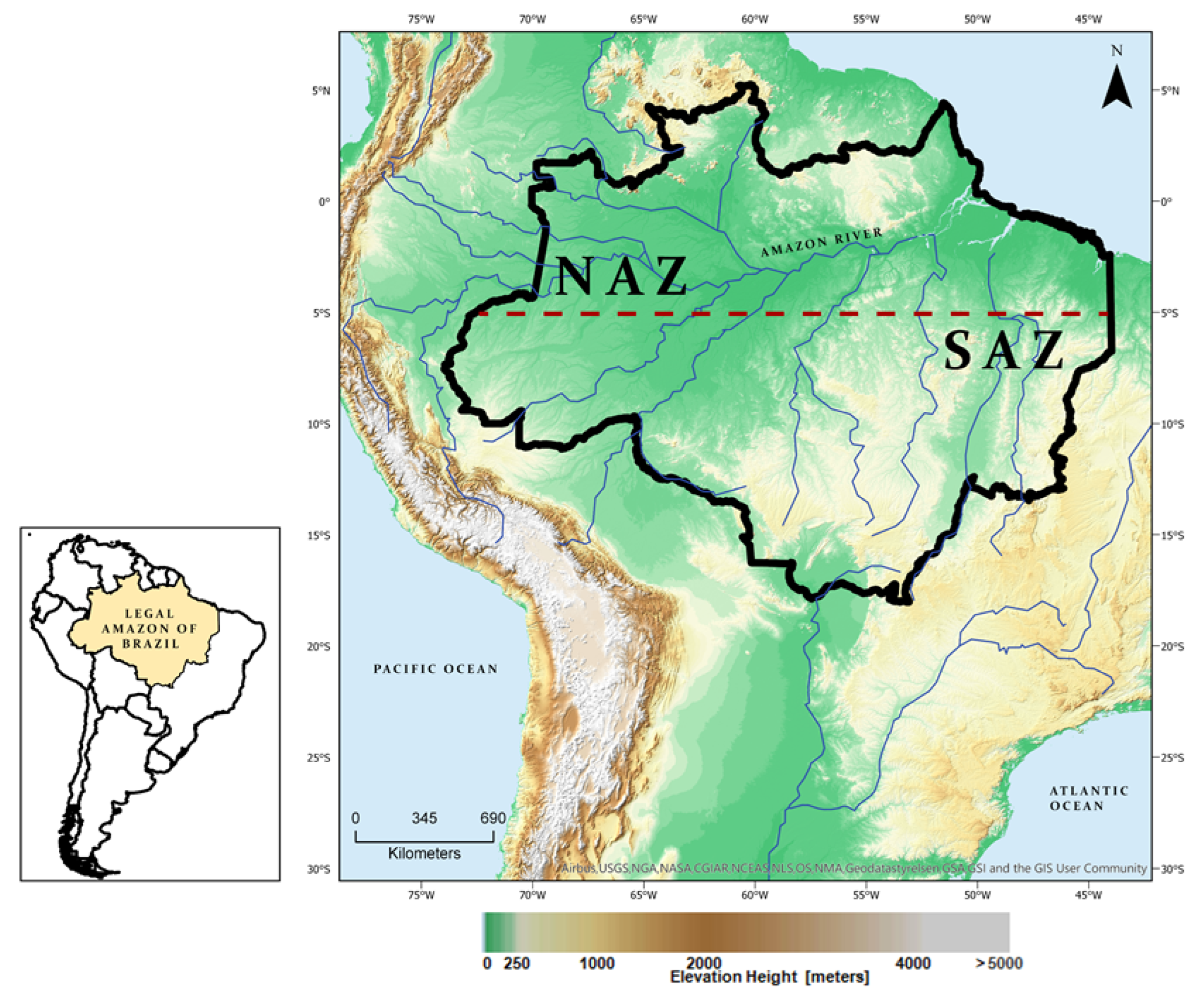
The Brazilian Amazon (Figure 1) is the portion of Brazil which encompasses the Amazon Rainforest, two-thirds of which lies in Brazil. The Brazilian Amazon contains mainly zone A with Af (without dry season), Am (monsoon), Aw (with dry winter), and the very eastern portion of the Brazilian Amazon contains As (with a dry summer) and BSh (semi-arid, low latitude and altitude), according to Köppen climate classification. This region is important for carbon and oxygen cycles, moisture dynamics, natural resources, species diversity, and many more ecosystem services. However, this region has lost over 107,000 km2 of forest, with some states losing close to 40,000 km2 or 42% of their entire forest composition since 2008 [39]. Most of the deforestation is due to cropland creation or other agriculture practices and has significant implications for changes in the precipitation regime [40,41,42,43]. In general, a clearing of forests leads to a drying of the region with less evapotranspiration and higher temperatures. However, results are still uncertain for many areas of the Brazilian Amazon. Therefore, it is very important to understand historical precipitation regime and to evaluate climate model capabilities to simulate the rainfall patterns for this region. In addition to a domain-wide analysis, this study will analyze a split domain for the Brazilian Amazon including a northern (NAZ) and southern (SAZ) Amazon focus (Figure 1). These regions have well-identified seasonal cycles of precipitation and consist of similar climate structures and have been used in other regional analyses of South America [32,44].
2.2. Observational Datasets
A total of three observational datasets will be used to evaluate CMIP6 model results. The primary dataset will be the Climate Hazards Group Infrared with Station data (CHIRPS), which contains 35 years of quasi-rainfall data that combine both satellite imagery and station data to create a rainfall time series [45]. The second will be the University of Delaware (UDEL) which contains long-term datasets from 1900 using station data of monthly total rain gauge-measured precipitation [46]. The third is CPC Merged Analysis of Precipitation (CMAP) which contains five kinds of satellite estimates (GPI, OPI, SSM/I scattering, SSM/I emission, and MSU) and rain gauge data [47]. In addition, Global Land Data Assimilation System (GLDAS) precipitation and evapotranspiration (ET) and 20th Century Reanalysis v2C (20cRv2C) surface pressure, specific humidity, meridional, and zonal wind data are used to analyze moisture flux convergence (MFC) ratio (precipitation/ET) biases. GLDAS relies on satellite and ground-based observational products and produces land surface states and flux datasets from land surface modeling and data assimilation, while 20cRv2C relies on a combination of observations rerun with the National Center for Environmental Protection Global Forecast System 2008ex model with 28 pressure levels and updated physical parameterizations [48,49,50,51,52,53,54]. All datasets were used for model evaluation comparison and contain data from 1981 to 2014. When only one observational dataset is needed for evaluation, CHIRPS is used because it represents one of the best rain-gauge substitutes for precipitation datasets [55].
2.3. CMIP6 Models
Ref. [25] provide a thorough overview of the Coupled Model Intercomparison Phase 6 (CMIP6) models and address the experimental design and organization of all experiments and simulations conducted. The models represent the most up-to-date climate model simulations for the climate science community. Ref. [25] concluded that the results from the CMIP6 experiments will represent the best global representation of past and future climate and lead to many significant advances for climate science and the science community at large.
This study uses a subset of 13 CMIP6 models to evaluate the representation of the historical Brazilian Amazon precipitation regime for 1981–2014. Model types include atmosphere-ocean general circulation models (AOGCM) with additional model components, such as aerosols (AER), chemistry (CHEM), and biogeochemistry (BGC). Table 1 presents the 13 models, their type, and corresponding institution, and location. The historical experiment was used for evaluating precipitation, as this experiment is traditionally used when compared to observational datasets . A total of three members from each model were selected to create an ensemble mean used in evaluation. SAM0UNICON was the exception and only contained one member which was used as the mean for this model. To keep datasets consistent, all models were regridded to 0.25° × 0.25° using bilinear interpolation. This method has been used for model evaluation in South America in multiple studies [33,56]. It has been found that using other methods, like nearest-neighbor, did not significantly improve the results [33].
2.4. Evaluation Methodology
To evaluate the ability of CMIP6 models to simulate the historical precipitation regime for the Brazilian Amazon, results were compared to observations for the period 1981–2014. We selected this period because it incorporates recent updates in the global telecommunications system and recent satellite-derived improvements in data collection. To evaluate annual cycles, we used the statistical metrics: root mean square error (RMSE), bias, and the spatial and temporal Pearson correlation coefficient. Both the monthly averages and anomalies of precipitation were evaluated. We also included analysis of precipitation extremes using the cumulative distribution function. A Taylor diagram was produced for the entire Brazilian Amazon, to give an overall idea of model performance for the region.
In addition to the model performance comparison, we performed EOF analysis to characterize the precipitation intraseasonal variability of the 13 CMIP6 models. To quantify the EOF eigenvector sampling error, we used the method described in [66]. Finally, the Taylor skill score [67,68], was used to give an overview of model performance (Equation (1)). Here S is the skill score, R is the correlation between the simulated and reference datasets, is the theoretical maximum correlation (assumed to be 1), and is the standard deviation of the simulated dataset.
3. Results and Discussion
3.1. Domain Analysis
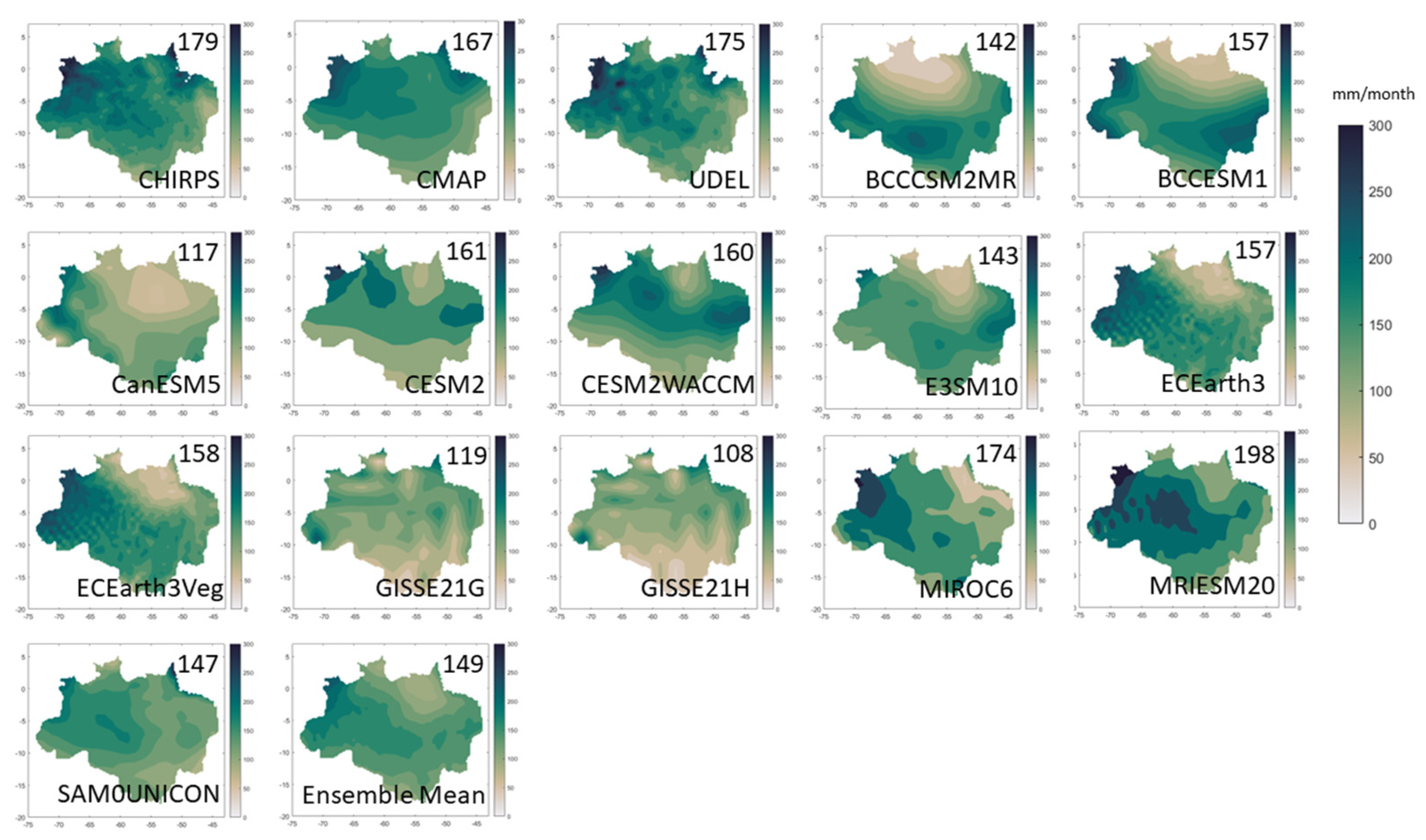
Spatial monthly mean averages for the three observational datasets and all 13 GCMs from 1981 to 2014 are shown in Figure 2. Observed rainfall shows wetter conditions in the northeast and northwest along the equatorial latitude and dry conditions in the southern and eastern sections of the domain. The mean values for the entire Brazilian Amazon range from 167 mm month−1 to 179 mm month−1 for the observed datasets while models range from 108 mm month−1 to 198 mm month−1. Most models display a much drier condition in the north and northeast portion of the study region with monthly averages below 60 mm month−1, except for MRIESM20 and SAM0UNICON. MIROC6 and MRIESM20 appear to overestimate precipitation patterns west of 55° W and north of 10° S with averages of 250 or more mm month−1, while observation shows monthly values closer to 150–200 mm month−1. CanESM5 shows the driest northern bias when compared to observation, with much of the northeastern portion showing values of around 50 mm month−1. GISSE21G and GISSE21H show scattered dry biases throughout the entire domain, especially in the southern region with values closer to 50 mm month−1 compared to 100–150 mm month−1 in the observed domain. The ensemble mean and SAM0UNICON show the best spatial representation of precipitation with no large dry biases and a uniform state of precipitation throughout the study domain, although the ensemble mean has a dry bias in the north due to most models underestimating precipitation here.
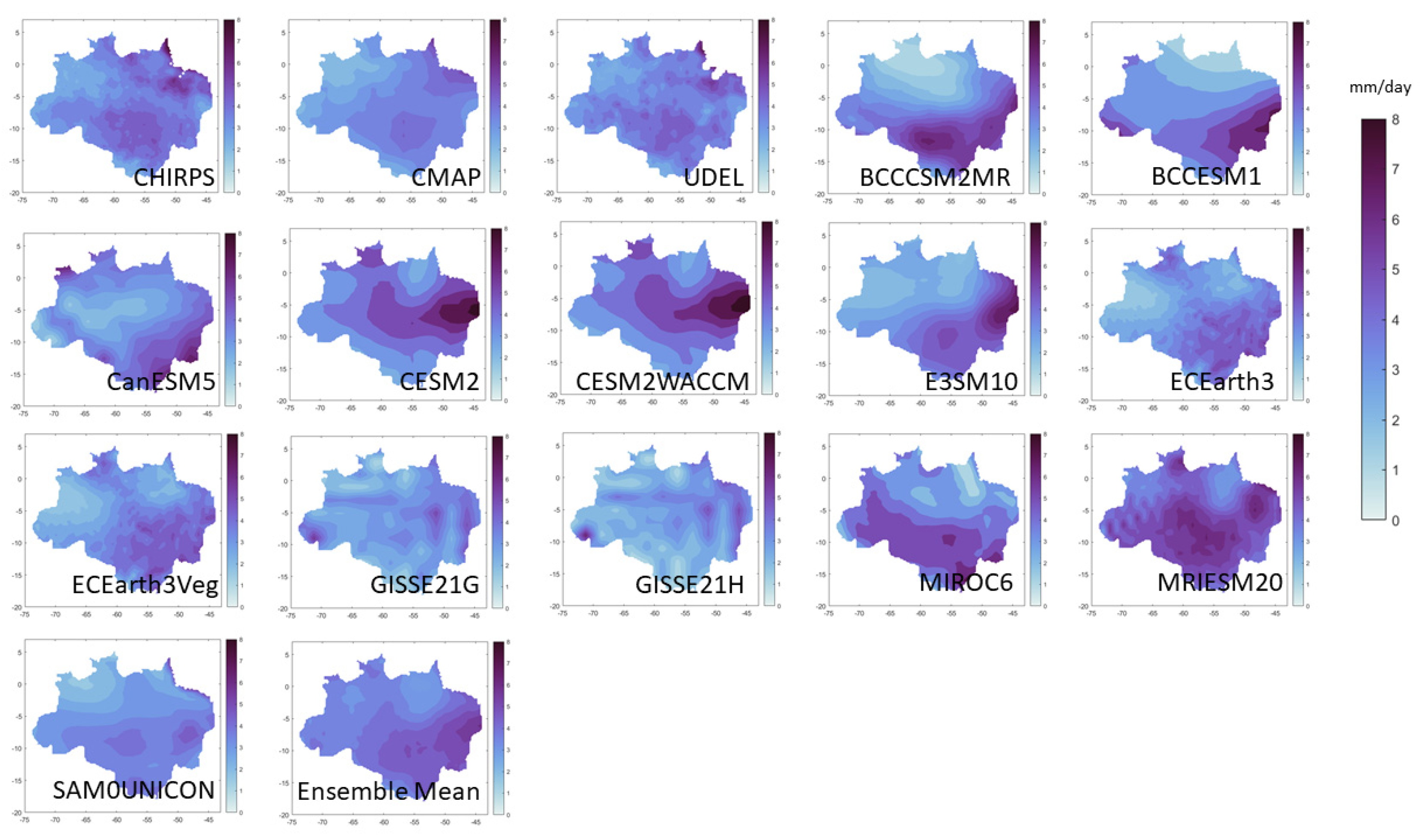
To test for model performance of precipitation variability, monthly standard deviation of all monthly values for each dataset is shown in Figure 3 in mm day−1 for 1981–2014. The mean seasonal cycle was not subtracted from each dataset and therefore these values include both the seasonal cycle and interannual variability. CHIRPS and UDEL show very similar spatial characteristics with higher variability in the southern and northeastern portions of the study domain of up to 8 mm day−1, while CMAP shows less variability overall of a few mm. Models that show lower variability in the northern Brazilian Amazon include BCCCSM2MR, BCCESM1, E3SM10, ECEarth3, ECEarth3Veg, GISSE21G, GISSE21H, and MIROC6. BCCCSM2MR, E3SM10, MIROC6, and MRIESM20 show higher variability by 3–4 mm day−1 in the southern portion of the domain. Models that show higher variability in the eastern region, along the coastal portions of the domain include BCCESM1, CESM2, CESM2WACCM, E3SM10, MRIESM20, and the ensemble mean. Again, based on spatial mean analysis of the entire period, SAM0UNICON and the ensemble mean produced the best representation of mean monthly precipitation standard deviation.
The Taylor diagram provides information on the normalized standard deviation, centered root mean square error, and the correlation coefficient of the monthly values for each model, CMIP6 ensemble mean, CMIP5 ensemble mean, CMAP, and UDEL with a reference dataset for the entire Brazilian Amazon (Figure 4). This analysis allows for a general comparison of all datasets for the whole study domain. The reference observation dataset used in this analysis is CHIRPS. In general, models and the two additional observational datasets performed adequately when compared to CHIRPS. The CMIP6 ensemble mean has outperformed the previous suite of CMIP5 models in terms of standard deviation. CMIP6 models have become less variable from observation than previous models. All models had a correlation coefficient above 0.8 and had a standard deviation between 0.5 and 1.5. The best performance was the ensemble mean, with SAM0UNICON, GISSE21G, and E3SM10 close to the reference dataset. From this diagram, the models that overestimated rainfall for this period were MIROC6, CESM2, CES2WACCM, and MRIESM20. Models that underestimated domain average precipitation were the ensemble mean, GISSE21G, SAM0UNICON, E3SM10, GISSE21H, BCCCSM2MR, CanESM5, ECEarth3Veg, ECEarth3, and BCCESM1. Models that had a high correlation around 0.92 but high standard deviation of about 1.3 were CESM2, CESM2WACCM, and MRIESM20. The model with the highest correlation coefficient is the ensemble mean with a value of 0.93 and the model with the lowest value is BCCESM1 at 0.82. The ensemble mean performed best for the entire Brazilian Amazon.
3.2. Northern (NAZ) and Southern (SAZ) Amazon Regions
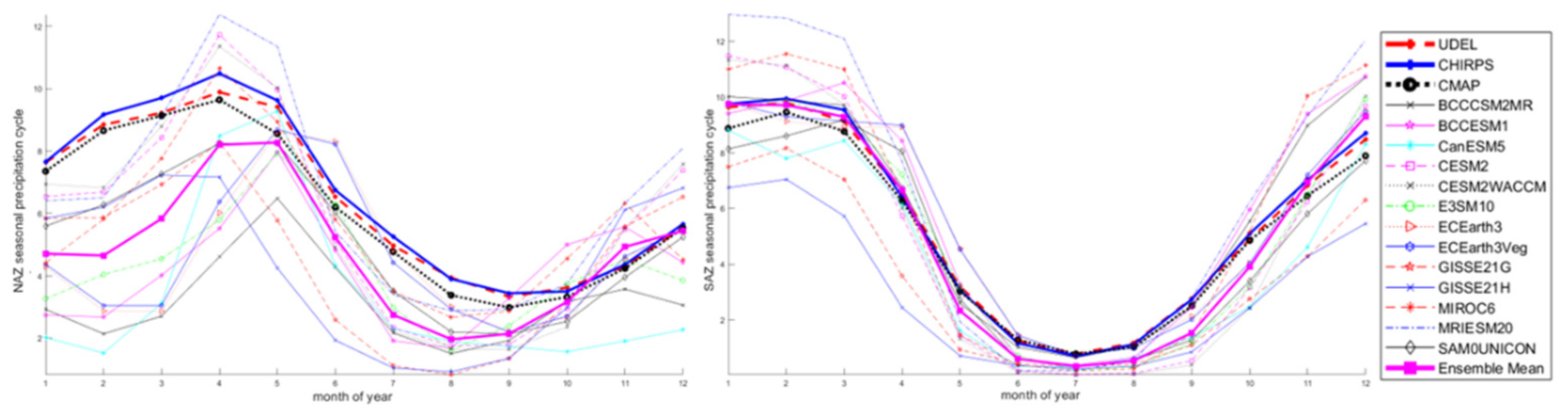
The climate of the Brazilian Amazon is characterized by monsoonal climate with a marked dry and wet season cycle. Typically, the dry season runs from June to August (JJA) and the wet season from December to February (DJF). SAZ modeled results have a defined dry and wet season (observational dataset values range from 1.5 to 10 mm day−1 and model values range from 1 to 13 mm day−1) when compared to NAZ (observational dataset values range from 3.5 to 10 mm day−1 and model values range from 1 to 12 mm day−1) (Figure 5). SAZ has a dry season in JJA and a wet season in DJF, while NAZ has a dry season in ASO and a wet season in MAM according to the observed datasets. For NAZ, models tend to underestimate precipitation during the dry season and the wet season, except for CESM2, CESM2WACCM, and MRIESM20 which overestimate precipitation during the peak of the wet season by up to 2 mm day−1. Some models underestimate wet season precipitation up to 7.5 mm day−1. Ensemble mean for NAZ performs best for the beginning and the end of the wet season but underestimates precipitation during peak wet and dry season. For SAZ, models were able to capture the progression of the wet and dry season with higher accuracy, although the range of modeled values is 1 to 13 mm day−1 where the observational dataset range is only 1.5 to 10 mm day−1. Most models underestimate dry season precipitation for SAZ, by about 0.5 mm day−1. Models capture the timing of the wet season but disagree during the peak of the wet season and both over- and under-estimate precipitation. During JFM (peak wet season for SAZ), observational datasets deviate about 1 mm day−1, while model values range between 5 mm day−1. Ensemble mean for SAZ performs best. Overall, models were able to capture the dry and wet season cycles, although the performance was more accurate for the SAZ compared to NAZ climatology. Most models underestimate dry and wet season precipitation, although wet season modeled results are more variable. Models can capture the dry season progression especially well for SAZ.
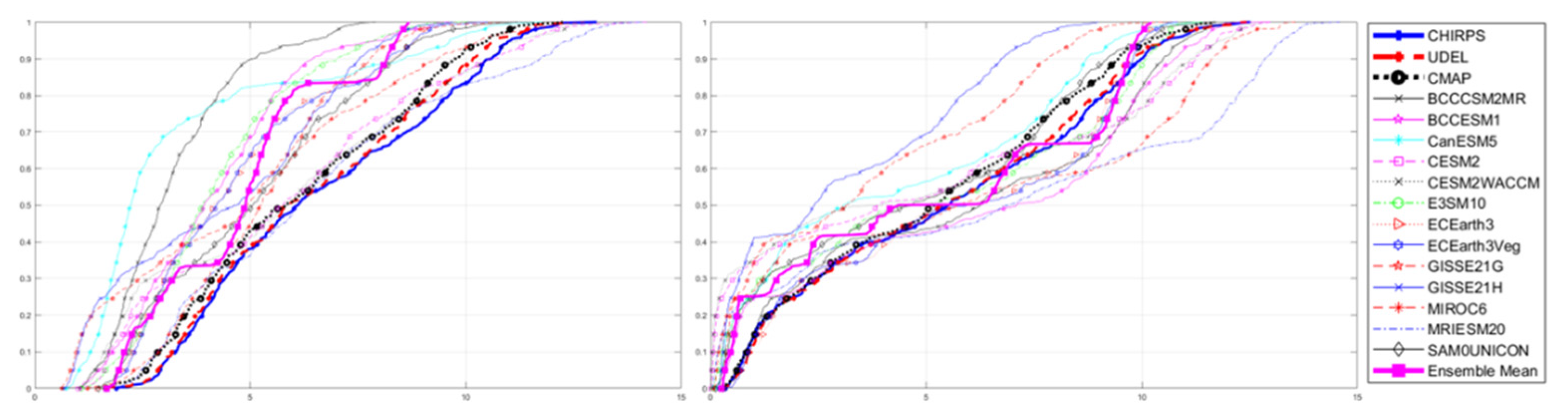
Cumulative distribution function (CDF) results in Figure 6 are used to identify whether models can capture extreme precipitation (minimum and maximum feature in the CDF). In general, models underestimate NAZ precipitation especially BCCCSM2MR and MRIESM20. Ensemble mean captures NAZ minimum precipitation values well and exhibits clustering effects around 3 to 4 mm day−1 and 6 to 8 mm day−1 but does not capture maximum precipitation. The models that capture NAZ maximum precipitation are CanESM5, CESM2, CESM2WACCM, GISSE21G. GISSE21H overestimates NAZ maximum precipitation. Models capture SAZ minimum precipitation very well because SAZ is drier and contains many observations of no rainfall, therefore models capture the minimum value of observations well. Most models underestimate SAZ precipitation up to a threshold of 5 mm day−1 but then diverge after this value and exhibit over- and under-estimation of higher precipitation observations. The ensemble mean performs relatively well, although clustering effects occur more often for SAZ than NAZ. Models both over- and under-estimate maximum precipitation with BCCESM1, BCCCSM2MR, ECEarth3Veg, and E3SM10 capturing the right tail best. CESM2, CESM2WACCM, MRIESM20, and MIROC6 all overestimate SAZ maximum precipitation. Overall, MRIESM20 follows the distribution of NAZ best, despite its overestimation of extreme precipitation while ECEarth3Veg follows the distribution of SAZ best, although it overestimates precipitation values from 5 to 8 mm day−1. Ensemble mean follows the distribution of SAZ better than NAZ, although it exhibits clustering effects.
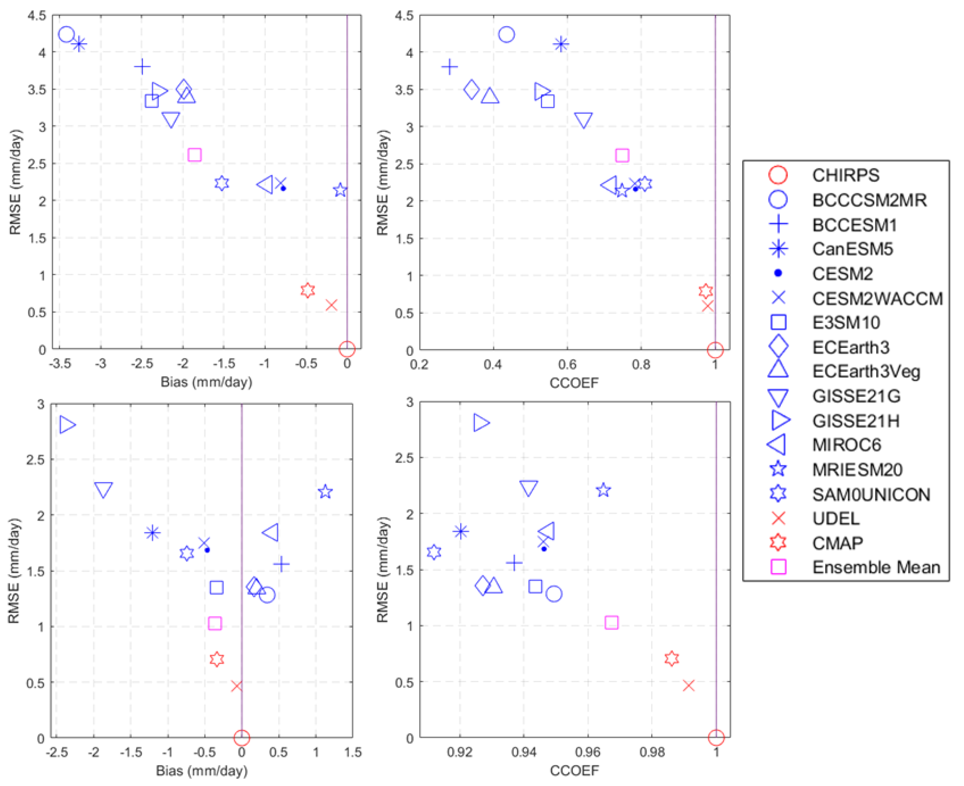
RMSE-bias and RMSE-correlation coefficient diagrams further illustrate the relationship between these performance metrics for the models (Figure 7). For NAZ domain, MRIESM20, CESM2, CESM2WACCM, MIROC6, and SAM0UNICON performed the best with an approximate RMSE of 2.25 mm day−1, a bias ranging from −1.5–0.2, and an approximate correlation coefficient of 0.75. For SAZ, the best performing models were the ensemble mean, BCCCSM2MR, E3SM10, ECEarth3, ECEarth3Veg, BCCESM1, CESM2, CESM2WACCM, MIROC6, and SAM0UNICON. CESM2, CESM2WACCM, MIROC6, and SAM0UNICON were also some of the best performing models for NAZ. The top five performing models for SAZ had an approximate RMSE of 1.27 mm day−1, a bias ranging from −0.36 to +0.34, and a correlation coefficient of 0.95. Models had a larger RMSE for NAZ with the largest RMSE error +1.4 mm day−1 greater than the largest RMSE for SAZ. In addition, biases for both NAZ and SAZ showed a similar range with biases ranging 3.5 mm day−1. Errors were larger for NAZ, as models tended to underestimate precipitation here. Biases are less systematic in SAZ. Overall, the top models include CESM2, CESM2WACCM, MIROC6, SAM0UNICON, BCCCSM2MR, E3SM10, BCCESM1, ECEarth3, ECEarth3veg, and the ensemble mean. However, BCCCSM2MR, E3SM10, BCCESM1, ECEarth3, and ECEarth3Veg did not perform as well for NAZ.
3.3. EOF Analysis
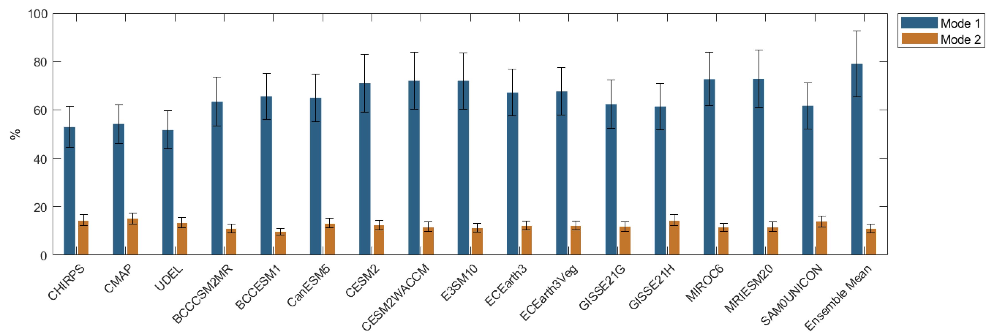
Only the two first modes of EOF analysis are described in this section as together they explain over 67% of the precipitation variability (Figure 8 and Figure 9).
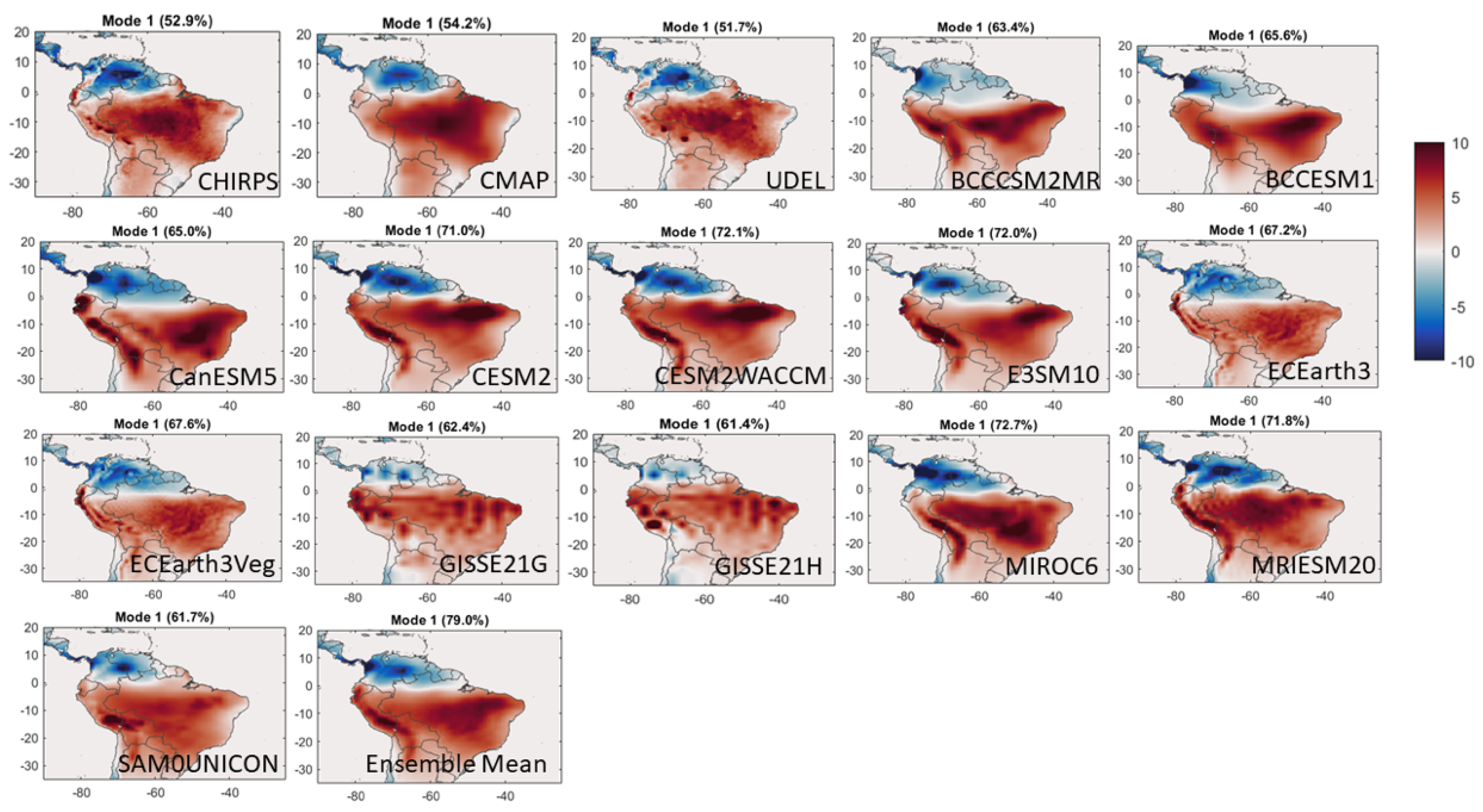
The first EOF (Figure 8) explains approximately 53% within observational datasets, and around 68% of the variability in CMIP6 models and follows a temporal pattern like the annual cycle of precipitation, with a dry season around JJA and a wet season mainly in the months of DJF. The eigenvector has a dipole structure with the zero line around the equator, reflecting the different temporal evolution of the SAMS between the northern and southern region. The SAMS is largely responsible for the annual cycle of precipitation and the SAMS’ temporal structure is confirmed from the PC time series (Figure 9). Overall, models capture this mode of variability well, although some models overestimate the precipitation over the Andes mountains on the western coast of South America. In addition, a too high fraction of the variability is explained by this eigenvector in the models, with a bias of up to +19.8% for MIROC6 and +26% for the ensemble mean.
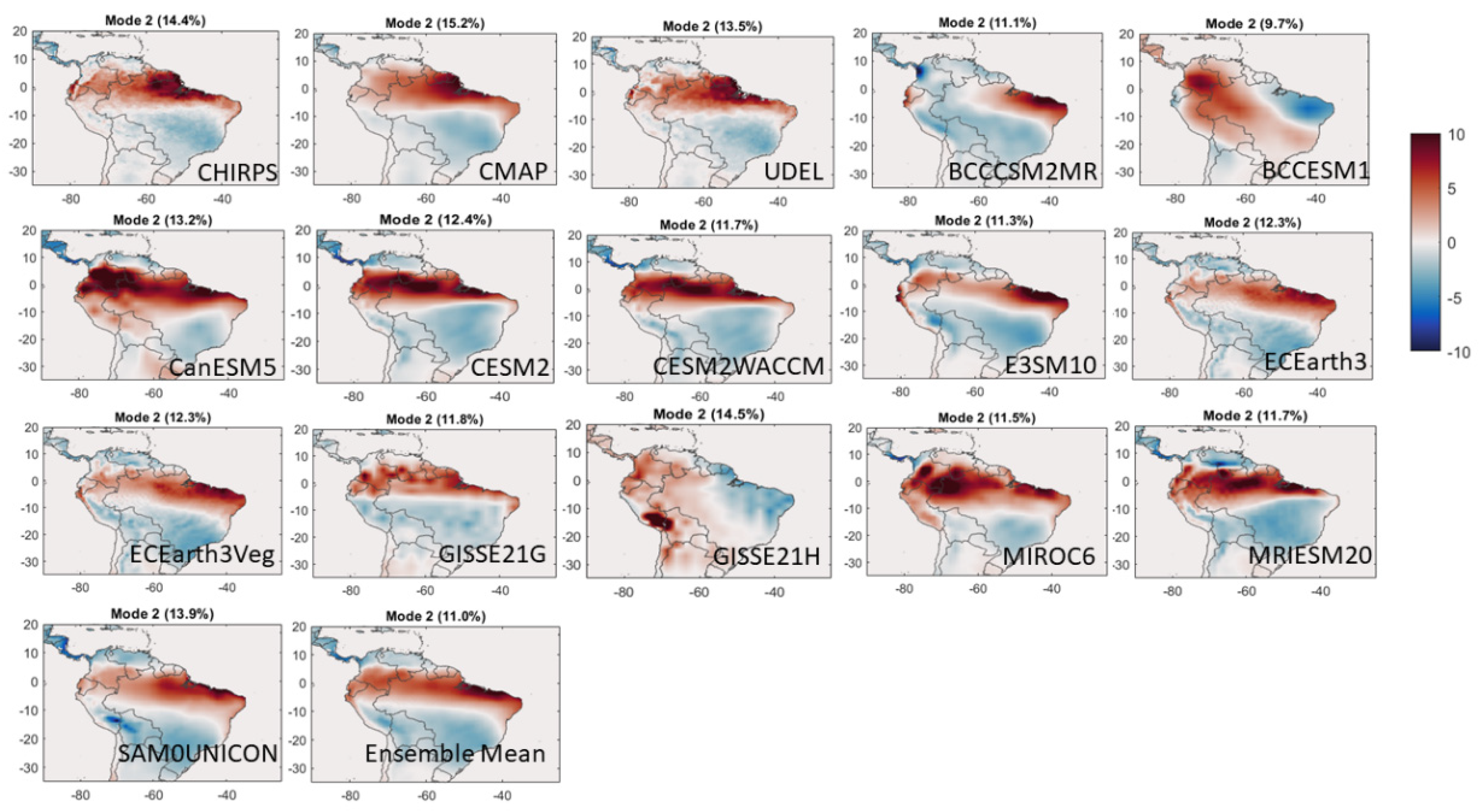
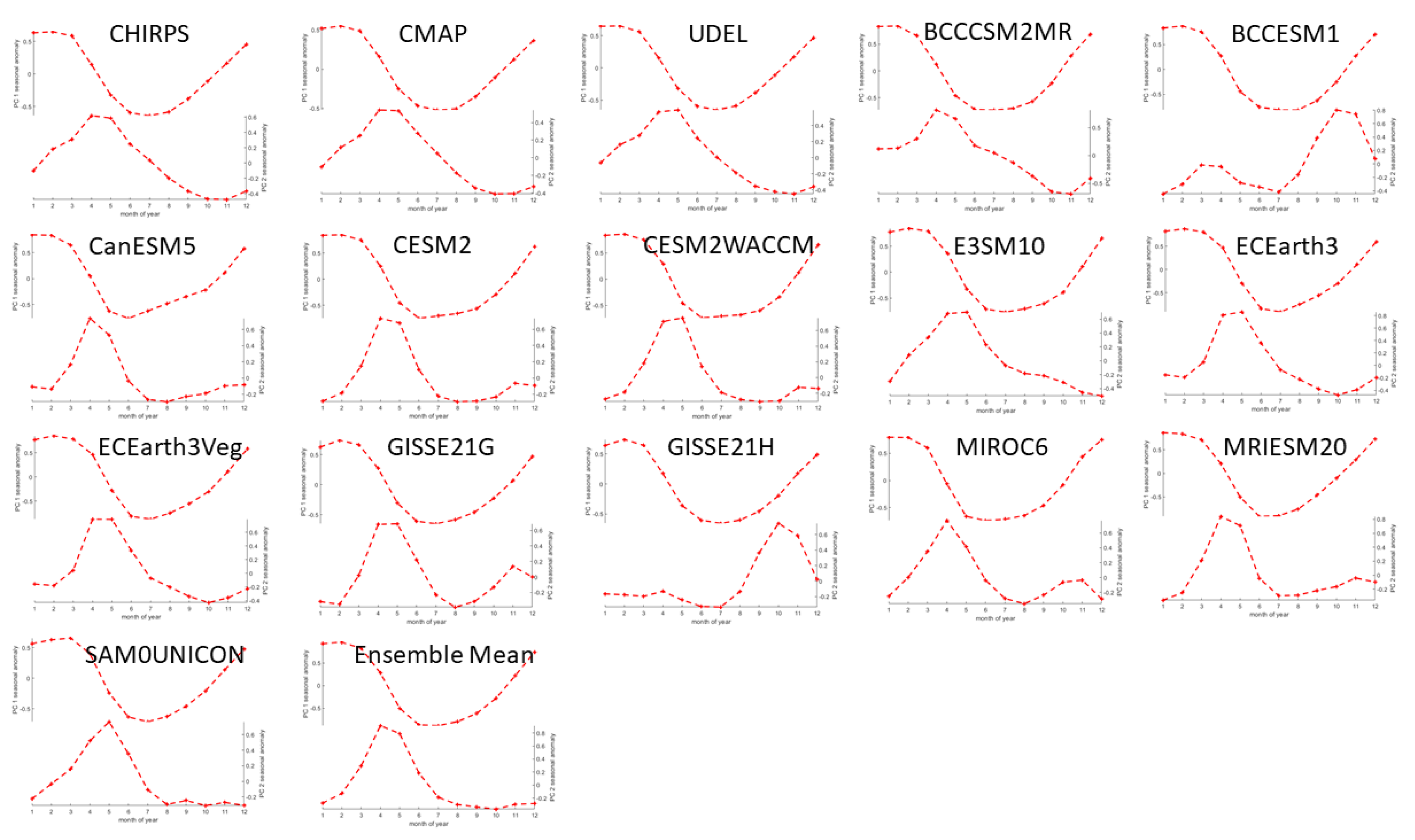
The second EOF explains approximately 14% (according to Figure 9) within the observational datasets while the CMIP6 models explain 2% less. This EOF explains the transition between the SAMS and the North American Monsoon System (NAMS) [69]. There is a tripole nature to this eigenvector with an out-of-phase band around −8° to 8° of latitude for the positive values, which represents how these two regions of South America differ in terms of the temporal evolution of the SAMS. The SAMS originates in the southeast portion of South America over the mountainous region of the Brazilian Highlands and moves northward over South America, bringing precipitation as it travels to North America. During austral winter (JJA) the ITCZ is dominant, with most of the precipitation in the northern region of South America and Brazil. This is the spatial pattern we are seeing in this second EOF. The PC time series (Figure 10) shows a delay in the onset of the wet season for this eigenvector with observation showing its onset around April and May and models showing a similar pattern, except for BCCESM1 and GISSE11H. This delay signals the time evolution of SAMS across the vast land area of Brazil. Models seem to capture the tripole nature of the transitional SAMS, excluding BCCSM2MR, BCCESM1, and GISSE21H. Models are more accurate in placing the correct fraction of explained variance (%) for this mode. CESM2, CESM2WAACCM, GISSE21G, MIROC6, MRIESM20, SAM0UNICON, and the ensemble mean appear to have captured the second eigenvector most accurately.
Overall, models were able to capture the seasonal cycle and dipole nature of SAMS, although the variance explained by the first mode was much higher for the models than for the observations: up to +26% for the ensemble mean (Figure 11). Average observation eigenvector 1 explained 3%, while the eigenvector 2 explained 9% of the variability. Models had a combined eigenvector 1 explanation of 67% (14% higher than observation) and 12% explanation for eigenvector 2 (3% higher than observation). Models had a difficult time simulating the temporal progression of the second mode of variability. However, some models, like CESM2, CESM2WAACCM, GISSE21G, MIROC6, MRIESM20, SAM0UNICON, and the ensemble mean, were able to simulate the mapped eigenvector well.
3.4. Taylor Skill Score and Ranking
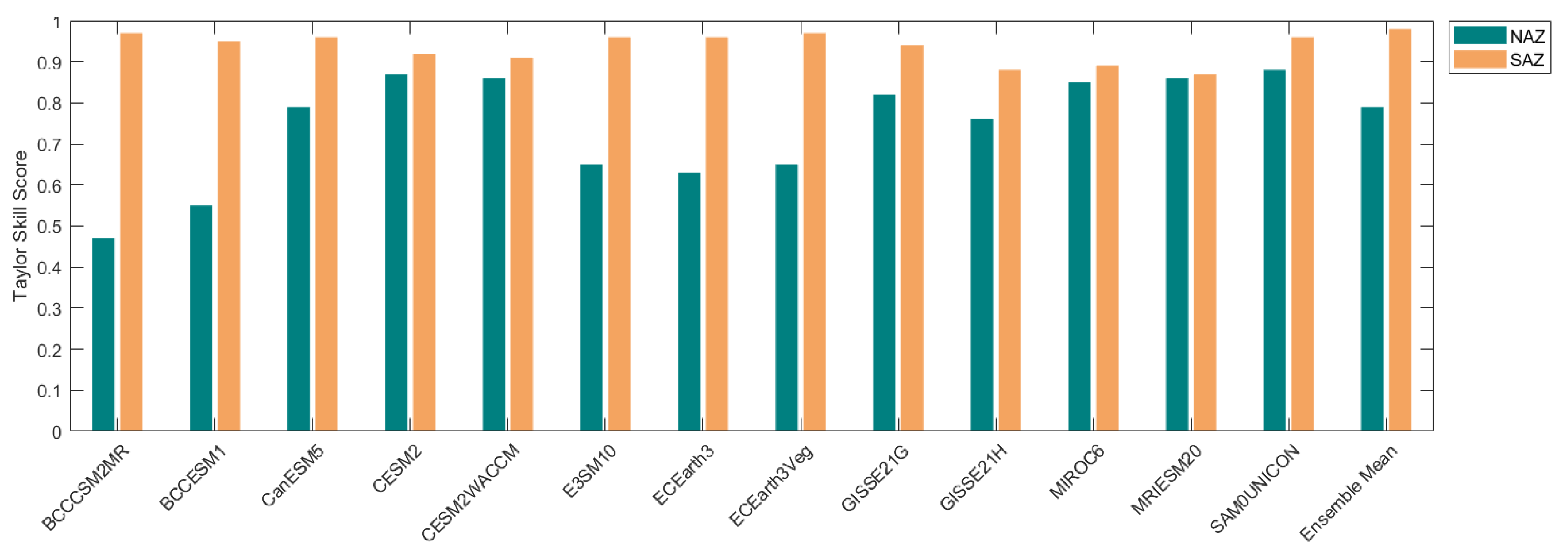
To evaluate overall model effectiveness, the Taylor skill score was calculated for all GCMs and the ensemble mean for both subdomains (Figure 12). Overall, models performed better in SAZ than in NAZ. All models for SAZ scored a 0.87 or better and the highest score was the ensemble mean with a score of 0.98. The top models for SAZ, according to Taylor skill score, are ECEarthVeg (0.97), BCCCSM2MR (0.97), CanESM5 (0.96), E3SM10 (0.96), E3SM10 (0.96), and SAM0UNICON (0.96). Performance was lower for NAZ with the scores ranging from 0.47 to 0.88. The models with the highest skill score for NAZ include SAM0UNICON (0.88), CESM2 (0.87), CESM2WACCM (0.86), MRIESM20 (0.86), and MIROC6 (0.85). The ensemble mean score for NAZ is 0.79, being the 7th highest. When both domains are considered, the top models are CESM2, CESM2WACCM, MIROC6, MRIESM20, and SAM0UNICON. When modelers take this into consideration, model ensembles can be constructed based on the highest performing GCMs for this region.
3.5. ET/PR & MFC/PR Ratio Analysis
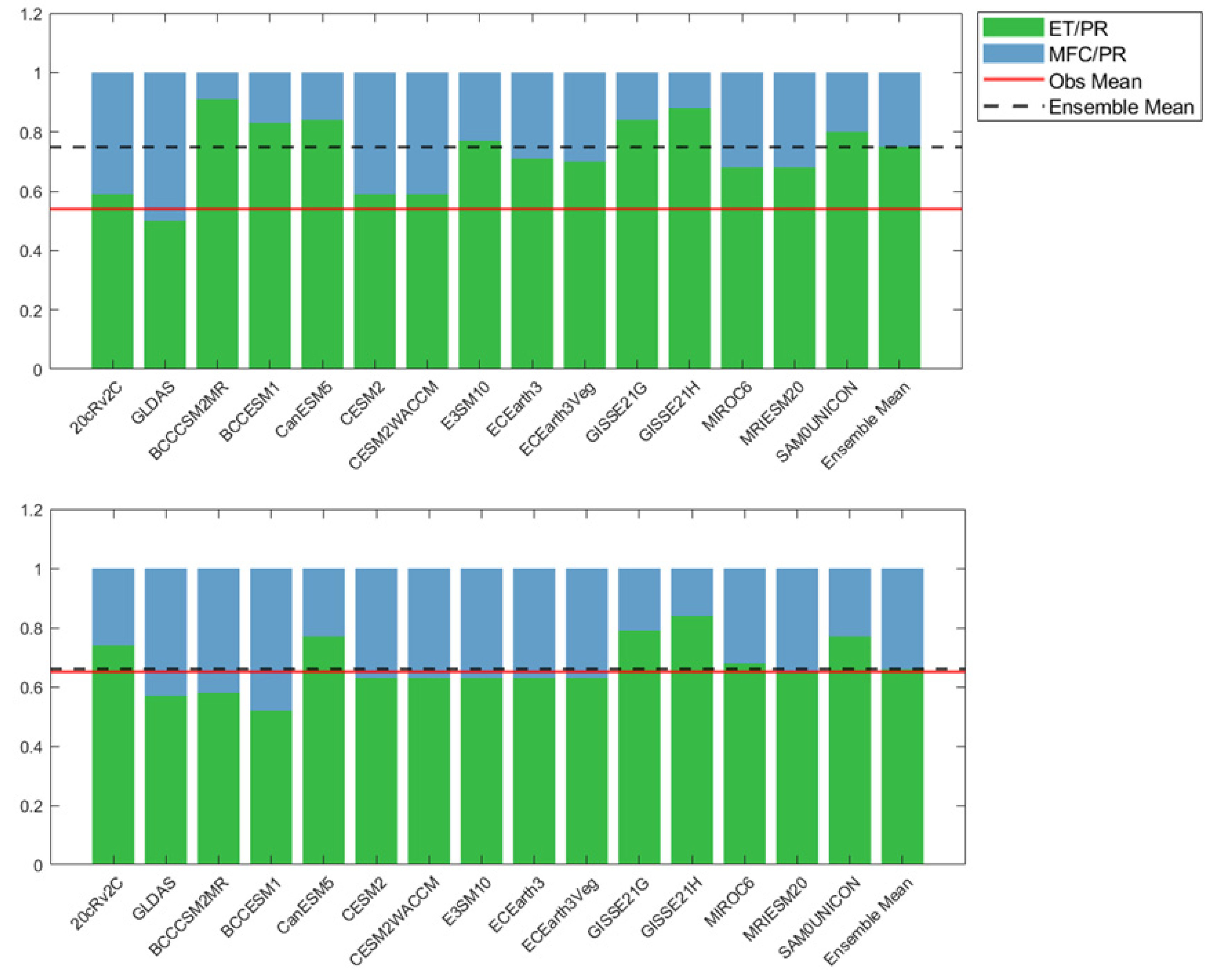
To explore GCM performances, we use ET/PR and MFC/PR ratio analysis to investigate how CMIP6 models partition the source of rainfall moisture between surface source (evapotranspiration) and atmospheric source (moisture flux convergence) for both northern and southern subdomains (Figure 13). Observations show that NAZ ET/PR ratio is lower than SAZ by an average of 0.11 and therefore there were greater amounts of MFC compared to ET values, when compared to SAZ. SAZ showed greater values of ET when compared to NAZ MFC ratio analysis for observations. Models show a higher average ET/PR mean by 0.21 for NAZ and 0.01 for SAZ. Models were better at capturing SAZ partition of precipitation sources between ET and MFC for 1981–2014 as the ET/PR ratio means were much closer to observed means.
For NAZ, the top performing models (based on the difference in ratio from the average of GLDAS and 20cRv2C ratio values) are CESM2 (0.05), CESM2WACCM (0.05), MIROC6 (0.14), MRIESM20 (0.14), ECEarth3 (0.17), and ECEarth3Veg (0.16). For SAZ, the top performing models (based on the difference in ratio from the average of GLDAS and 20cRv2C ratio values) are CESM2 (−0.02), CESM2WACCM (−0.02), E3SM10 (−0.02), ECEarth3 (−0.02), and ECEarth3Veg (−0.02), MRIESM20 (0.00), the ensemble mean (0.01) and MIROC6 (0.03).
Models tend to underestimate PR for both NAZ and SAZ (Figure 7). This analysis reveals that the precipitation in models is too strongly dominated by the ET source, resulting in ET/PR ratios larger than GLDAS and 20cRv2C with an average of 0.12. Despite generally higher values of simulated ET, the models might not be producing enough moisture from convergence flux to simulate PR accurately, resulting in low PR when compared to CHIRPS, CMAP, and UDEL. This is not the only research that has found that models tend to underestimate PR, as other studies have shown that CMIP models tend to underestimate precipitation in this region [35]. More work needs to be completed to analyze the physical mechanisms and schemes within each model which produce the biases in precipitation, ET, and MFC, which is beyond the scope of this paper. Understanding the underlying physics of each GCM is an important component of model evaluation, which individual modeling teams can contribute towards.
4. Conclusions
The Brazilian Amazon is an important region to study, as it provides a significant amount of resources, not just locally, but globally. The precipitation regime and the significance it represents for the people, environment, and ecosystem is one of the Amazon’s most significant ecosystem goods [70], and therefore should be studied and modeled properly. This study evaluates the ability of 13 CMIP6 GCMs to simulate precipitation for a historical period (1981–2014) for the Brazilian Amazon. The GCMs were selected from the historical experiment from the CMIP6 simulations and ensemble means were taken to suppress the effect of internal variability in the individual models. Simulations from GCMs are evaluated using spatial pattern mapping, Taylor diagram analysis and Taylor skill score, annual climatology comparison, and EOF analysis. Using multiple analysis metrics allows for a holistic approach to model evaluation, and no one model performed best for all analyses.
Precipitation analysis for the Brazilian Amazon (1981–2014) shows: (1) This region displays higher rainfall in the north-northwest and drier conditions in the south. Models tend to underestimate northern values or overestimate the central to northwest averages. (2) SAZ has a much more defined dry season (JJA) and wet season (DJF) and models are able to simulate this well. NAZ dry season tends to occur in ASO and the wet season occurs in MAM, and models are not able to capture the climatology as well. Models tend to produce too much rainfall at the start of the wet season and tend to either over- or under-estimate the dry season (although the ensemble mean captures the anomalies for SAZ very well). The ensemble mean for NAZ can simulate the wet season decline. (3) In addition, models struggle to capture extreme values of precipitation except when precipitation values are close to 0. (4) EOF analysis of GCMs was able to capture the dominant mode of variability, which is largely the annual cycle or SAMS. Some models tend to overestimate precipitation over the Andes and place too high a fraction of explained variance on the first eigenvector by up to 26% for the ensemble mean. The second mode showed a tripole difference and displays a transition from the SAMS to the NAMS, as there is a delay in the onset of the principal component time series, when compared to the first. (5) When all evaluation metrics are considered the models that perform best are CESM2, MIROC6, MRIESM20, SAM0UNICON, and the ensemble mean.
This paper supports research in determining the most up-to-date CMIP6 model performance of precipitation regime for 1981–2014 for the Brazilian Amazon, a place rich in ecosystem goods and services. These results will hopefully aid in understanding future projections of precipitation for the selected subset of models and allow modelers and scientists to create an ensemble of high-performing GCMs for further analysis, as precipitation plays a role in many sectors of the economy, including the ecosystem, agriculture, energy, and water security.
Author Contributions
Conceptualization, C.M. and F.D.S.; data curation, C.M.; formal analysis, C.M.; funding acquisition, F.D.S.; methodology, C.M., F.D.S. and C.J.; project administration, C.M.; supervision, F.D.S. and C.J.; validation, C.M. and F.D.S.; visualization, C.M.; writing—original draft, C.M.; writing—review and editing, C.M., F.D.S. and C.J. All authors have read and agreed to the published version of the manuscript.
Funding
This study is based upon work supported by the National Science Foundation under Grant BCS-1825046. C. Jones would like to thank the financial support from the National Science Foundation under grant AGS-1937899.
Data Availability Statement
Data for all Global Climate Models from the Coupled Model Intercomparison Project Phase 6 (CMIP6) can be downloaded from the World Climate Research Programme (WCRP) site: https://esgf-node.llnl.gov/search/cmip6/ (accessed on 20 July 2020). The main precipitation dataset, Climate Hazards Group InfraRed Precipitation with Station data (CHIRPS), can be accessed from the University of California Santa Barbara Climate Hazards Center site: https://www.chc.ucsb.edu/data (accessed on 15 September 2020). CPC Merged Analysis of Precipitation (CMAP) can be accessed here: https://psl.noaa.gov/data/gridded/data.cmap.html (accessed on 15 September 2020). and the University of Delaware (UDEL) Precipitation can be accessed here: https://psl.noaa.gov/data/gridded/data.UDel_AirT_Precip.html (accessed on 15 September 2020). Precipitation and evapotranspiration data from Global Land Data Assimilation System (GLDAS) can be found here: https://disc.gsfc.nasa.gov/datasets?keywords=GLDAS (accessed on 10 August 2021). Twentieth Century Reanalysis data for moisture flux convergence analysis can be found on the National Oceanic and Atmospheric Association’s Physical Sciences Laboratory site here: https://psl.noaa.gov/data/gridded/data.20thC_ReanV2c.pressure.mm.html (accessed on 10 August 2021).
Acknowledgments
Support for the Twentieth Century Reanalysis Project version 2c dataset (20cRv2C) is provided by the U.S. Department of Energy, Office of Science Biological and Environmental Research (BER), and by the National Oceanic and Atmospheric Administration Climate Program Office. The authors would like to acknowledge high-performance computing support from Cheyenne (doi:10.5056/D6RX99HX) provided by NCAR’s Computational and Information Systems Laboratory, sponsored by the National Science Foundation.
Conflicts of Interest
The authors declare no conflict of interest.
References
- Foley, J.A.; Asner, G.; Costa, M.; Coe, M.T.; DeFries, R.; Gibbs, H.K.; Howard, E.A.; Olson, S.; Patz, J.; Ramankutty, N.; et al. Amazonia revealed: Forest degradation and loss of ecosystem goods and services in the Amazon Basin. Front. Ecol. Environ. 2007, 5, 25–32. [Google Scholar] [CrossRef]
- de Lima, L.S.; Coe, M.T.; Filho, B.S.S.; Cuadra, S.V.; Dias, L.C.P.; Costa, M.H.; Lima, L.S.; Rodrigues, H.O. Feedbacks between deforestation, climate, and hydrology in the Southwestern Amazon: Implications for the provision of ecosystem services. Landsc. Ecol. 2014, 29, 261–274. [Google Scholar] [CrossRef] [Green Version]
- Hopkins, M.J.G. Modelling the known and unknown plant biodiversity of the Amazon Basin. J. Biogeogr. 2007, 34, 1400–1411. [Google Scholar] [CrossRef]
- Dale, V.H.; Pearson, S.M.; Offerman, H.L.; O’Neill, R.V. Relating Patterns of Land-Use Change to Faunal Biodiversity in the Central Amazon. Conserv. Biol. 1994, 8, 1027–1036. [Google Scholar] [CrossRef]
- Wu, M.; Schurgers, G.; Ahlström, A.; Rummukainen, M.; Miller, P.A.; Smith, B.; May, W. Impacts of land use on climate and ecosystem productivity over the Amazon and the South American continent. Environ. Res. Lett. 2017, 12, 054016. [Google Scholar] [CrossRef] [Green Version]
- Martinelli, L.A.; Victoria, R.L.; Sternberg, L.S.L.; Ribeiro, A.; Moreira, M.Z. Using stable isotopes to determine sources of evaporated water to the atmosphere in the Amazon basin. J. Hydrol. 1996, 183, 191–204. [Google Scholar] [CrossRef]
- Chambers, J.Q.; Higuchi, N.; Tribuzy, E.S.; Trumbore, S.E. Carbon sink for a century. Nature 2001, 410, 429. [Google Scholar] [CrossRef]
- Salati, E.; Vose, P.B. Amazon Basin: A System in Equilibrium. Science 1984, 225, 129–138. [Google Scholar] [CrossRef] [Green Version]
- Zemp, D.C.; Schleussner, C.-F.; Barbosa, H.M.J.; van der Ent, R.J.; Donges, J.F.; Heinke, J.; Sampaio, G.; Rammig, A. On the importance of cascading moisture recycling in South America. Atmos. Chem. Phys. 2014, 14, 13337–13359. [Google Scholar] [CrossRef] [Green Version]
- Krol, M.S.; Bronstert, A. Regional integrated modelling of climate change impacts on natural resources and resource usage in semi-arid Northeast Brazil. Environ. Model Softw. 2007, 22, 259–268. [Google Scholar] [CrossRef]
- Parry, M.L.; Rosenzweig, C.; Iglesias, A.; Livermore, M.; Fischer, G. Effects of climate change on global food production under SRES emissions and socio-economic scenarios. Glob. Environ. Chang. 2004, 14, 53–67. [Google Scholar] [CrossRef]
- Hecht, S.B. Environment, development and politics: Capital accumulation and the livestock sector in Eastern Amazonia. World Dev. 1985, 13, 663–684. [Google Scholar] [CrossRef]
- Pedlowski, M.A.; Dale, V.H.; Matricardi, E.A.T.; da Silva Filhod, E.P. Patterns and impacts of deforestation in Rondônia, Brazil. Landsc. Urban Plan. 1997, 38, 149–157. [Google Scholar] [CrossRef]
- Fearnside, P. Deforestation of the Brazilian Amazon. In Oxford Research Encyclopedia of Environmental Science; Oxford University Press: New York, NY, USA, 2017. [Google Scholar] [CrossRef] [Green Version]
- Jones, C.; Carvalho, L.M.V. Climate change in the South American monsoon system: Present climate and CMIP5 projections. J. Clim. 2013, 26, 6660–6678. [Google Scholar] [CrossRef] [Green Version]
- Soares-Filho, B.; Rodrigues, H.; Follador, M. A hybrid analytical-heuristic method for calibrating land-use change models. Environ. Model. Softw. 2013, 43, 80–87. [Google Scholar] [CrossRef]
- Rodrigues, M.A.M.; Garcia, S.R.; Kayano, M.T.; Calheiros, A.J.P.; Andreoli, R.V. Onset and demise dates of the rainy season in the South American monsoon region: A cluster analysis result. Int. J. Climatol. 2021, 42, 1354–1368. [Google Scholar] [CrossRef]
- Sena, E.T.; Dias, M.A.F.S.; Carvalho, L.M.V.; Dias, P.L.S. Reduced wet-season length detected by satellite retrievals of cloudiness over Brazilian Amazonia: A new methodology. J. Clim. 2018, 31, 9941–9964. [Google Scholar] [CrossRef]
- Prado, L.F.; Wainer, I.; Yokoyama, E.; Khodri, M.; Garnier, J. Changes in summer precipitation variability in central Brazil over the past eight decades. Int. J. Climatol. 2021, 41, 4171–4186. [Google Scholar] [CrossRef]
- Smyth, J.E.; Ming, Y. Characterizing drying in the south American monsoon onset season with the moist static energy budget. J. Clim. 2021, 33, 9735–9748. [Google Scholar] [CrossRef]
- Erfanian, A.; Wang, G.; Fomenko, L. Unprecedented drought over tropical South America in 2016: Significantly under-predicted by tropical SST. Sci. Rep. 2017, 7, 5811. [Google Scholar] [CrossRef] [Green Version]
- Jiménez-Muñoz, J.C.; Mattar, C.; Barichivich, J.; Santamaría-Artigas, A.; Takahashi, K.; Malhi, Y.; Sobrino, J.A.; van der Schrier, G. Record-breaking warming and extreme drought in the Amazon rainforest during the course of El Niño 2015–2016. Sci. Rep. 2016, 6, 33130. [Google Scholar] [CrossRef] [PubMed] [Green Version]
- Chaudhari, S.; Pokhrel, Y.; Moran, E.; Miguez-Macho, G. Multi-decadal hydrologic change and variability in the Amazon River basin: Understanding terrestrial water storage variations and drought characteristics. Hydrol. Earth Syst. Sci. 2019, 23, 2841–2862. [Google Scholar] [CrossRef] [Green Version]
- Duffy, P.B.; Brando, P.; Asner, G.P.; Field, C.B. Projections of future meteorological drought and wet periods in the Amazon. Proc. Natl. Acad. Sci. USA 2015, 112, 13172–13177. [Google Scholar] [CrossRef] [Green Version]
- Eyring, V.; Bony, S.; Meehl, G.A.; Senior, C.A.; Stevens, B.; Stouffer, R.J.; Taylor, K.E. Overview of the Coupled Model Intercomparison Project Phase 6 (CMIP6) experimental design and organization. Geosci. Model. Dev. 2016, 9, 1937–1958. [Google Scholar] [CrossRef] [Green Version]
- Taylor, K.E.; Stouffer, R.J.; Meehl, G.A. An overview of CMIP5 and the experiment design. Bull. Am. Meteorol. Soc. 2012, 93, 485–498. [Google Scholar] [CrossRef] [Green Version]
- Chen, H.; Sun, J.; Lin, W.; Xu, H. Comparison of CMIP6 and CMIP5 models in simulating climate extremes. Sci. Bull. 2020, 65, 1415–1418. [Google Scholar] [CrossRef]
- Gusain, A.; Ghosh, S.; Karmakar, S. Added value of CMIP6 over CMIP5 models in simulating Indian summer monsoon rainfall. Atmos. Res. 2020, 232, 104680. [Google Scholar] [CrossRef]
- Zamani, Y.; Hashemi Monfared, S.A.; Azhdari moghaddam, M.; Hamidianpour, M. A comparison of CMIP6 and CMIP5 projections for precipitation to observational data: The case of Northeastern Iran. Theor. Appl. Climatol. 2020, 142, 1613–1623. [Google Scholar] [CrossRef]
- Chen, C.A.; Hsu, H.H.; Liang, H.C. Evaluation and comparison of CMIP6 and CMIP5 model performance in simulating the seasonal extreme precipitation in the Western North Pacific and East Asia. Weather Clim. Extrem. 2021, 31, 100303. [Google Scholar] [CrossRef]
- Li, J.-L.F.; Xu, K.-M.; Richardson, M.; Lee, W.-L.; Jiang, J.H.; Yu, J.-Y.; Wang, Y.-H.; Fetzer, E.; Wang, L.-C.; Stephens, G.; et al. Annual and seasonal mean tropical and subtropical precipitation bias in CMIP5 and CMIP6 models. Environ. Res. Lett. 2019, 15, 124068. [Google Scholar] [CrossRef]
- Alves, L.M.; Chadwick, R.; Moise, A.; Brown, J.; Marengo, J.A. Assessment of rainfall variability and future change in Brazil across multiple timescales. Int. J. Climatol. 2020, 41, E1875–E1888. [Google Scholar] [CrossRef]
- Rivera, J.A.; Arnould, G. Evaluation of the ability of CMIP6 models to simulate precipitation over Southwestern South America: Climatic features and long-term trends (1901–2014). Atmos. Res. 2020, 241, 104953. [Google Scholar] [CrossRef]
- Lovino, M.A.; Müller, O.V.; Berbery, E.H.; Müller, G.V. Evaluation of CMIP5 retrospective simulations of temperature and precipitation in northeastern Argentina. Int. J. Climatol. 2018, 38, e1158–e1175. [Google Scholar] [CrossRef]
- Gulizia, C.; Camilloni, I. Comparative analysis of the ability of a set of CMIP3 and CMIP5 global climate models to represent precipitation in South America. Int. J. Climatol. 2015, 35, 583–595. [Google Scholar] [CrossRef]
- Villamayor, J.; Ambrizzi, T.; Mohino, E. Influence of decadal sea surface temperature variability on northern Brazil rainfall in CMIP5 simulations. Clim. Dyn. 2018, 51, 563–579. [Google Scholar] [CrossRef]
- Barreto NDJ da, C.; Mendes, D.; Lucio, P.S. Sensitivity of the CMIP5 models to precipitation in Tropical Brazil. Rev. Ibero-Am. De Ciências Ambient. 2020, 12, 180–191. [Google Scholar] [CrossRef]
- Babaousmail, H.; Hou, R.; Ayugi, B.; Ojara, M.; Ngoma, H.; Karim, R.; Rajasekar, A.; Ongoma, V. Evaluation of the Performance of CMIP6 Models in Reproducing Rainfall Patterns over North Africa. Atmosphere 2021, 12, 475. [Google Scholar] [CrossRef]
- Assis, L.F.F.G.; Ferreira, K.R.; Vinhas, L.; Maurano, L.; Almeida, C.; Carvalho, A.; Rodrigues, J.; Maciel, A.; Camargo, C. TerraBrasilis: A Spatial Data Analytics Infrastructure for Large-Scale Thematic Mapping. ISPRS Int. J. Geo-Inform. 2019, 8, 513. [Google Scholar] [CrossRef] [Green Version]
- De Oliveira, G.; Brunsell, N.A.; Moraes, E.C.; Shimabukuro, Y.E.; Dos Santos, T.V.; Von Randow, C.; De Aguiar, R.G.; Aragao, L.E. Effects of land-cover changes on the partitioning of surface energy and water fluxes in Amazonia using high-resolution satellite imagery. Ecohydrology 2019, 12, e2126. [Google Scholar] [CrossRef]
- Khanna, J.; Medvigy, D.; Fueglistaler, S.; Walko, R. Regional dry-season climate changes due to three decades of Amazonian deforestation. Nat. Clim. Change 2017, 7, 200–206. [Google Scholar] [CrossRef]
- Bonini, I.; Rodrigues, C.; Dallacort, R.; Junior, B.H.M.; Carvalho, M.A.C. Rainfall and deforestation in the municipality of colider, Southern Amazon. Rev. Bras. Meteorol. 2014, 29, 483–493. [Google Scholar] [CrossRef] [Green Version]
- Butt, N.; De Oliveira, P.A.; Costa, M.H. Evidence that deforestation affects the onset of the rainy season in Rondonia, Brazil. J. Geophys. Res. Atmos. 2011, 116, D11120. [Google Scholar] [CrossRef]
- Nobre, C.A.; Sampaio, G.; Borma, L.S.; Carlos Castilla-Rubio, J.; Silva, J.S.; Cardoso, M. Land-use and climate change risks in the Amazon and the need of a novel sustainable development paradigm. Proc. Natl. Acad. Sci. USA 2016, 113, 10759–10768. [Google Scholar] [CrossRef] [PubMed] [Green Version]
- Funk, C.; Peterson, P.; Landsfeld, M.; Pedreros, D.; Verdin, J.; Shukla, S.; Husak, G.; Rowland, J.; Harrison, L.; Hoell, A.; et al. The climate hazards infrared precipitation with stations—A new environmental record for monitoring extremes. Sci. Data 2015, 2, 150066. [Google Scholar] [CrossRef] [Green Version]
- Willmott, C.J.; Matsuura, K. Global Air Temperature and Precipitation Archive. Available online: http://climate.geog.udel.edu/~climate/html_pages/README.ghcn_ts2.html (accessed on 18 June 2020).
- Xie, P.; Arkin, P.A. Global Precipitation: A 17-Year Monthly Analysis Based on Gauge Observations, Satellite Estimates, and Numerical Model Outputs. Bull. Am. Meteorol. Soc. 1997, 78, 2539–2558. [Google Scholar] [CrossRef]
- Compo, G.P.; Whitaker, J.S.; Sardeshmukh, P.D.; Matsui, N.; Allan, R.J.; Yin, X.; Gleason, B.E.; Vose, R.S.; Rutledge, G.K.; Bessemoulin, P.; et al. The Twentieth Century Reanalysis Project. Q. J. R. Meteorol. Soc. 2011, 137, 1–28. [Google Scholar] [CrossRef]
- Compo, G.P.; Whitaker, J.S.; Sardeshmukh, P.D. Feasibility of a 100-Year Reanalysis Using Only Surface Pressure Data. Bull. Am. Meteorol. Soc. 2006, 87, 175–190. [Google Scholar] [CrossRef] [Green Version]
- Hersbach, H.; Bell, B.; Berrisford, P.; Hirahara, S.; Horanyi, A.; Muñoz-Sabater, J.; Nicolas, J.; Peubey, C.; Radu, R.; Schepers, D.; et al. The ERA5 global reanalysis. Q. J. R. Meteorol. Soc. 2020, 146, 1999–2049. [Google Scholar] [CrossRef]
- Whitaker, J.S.; Compo, G.P.; Wei, X.; Hamill, T.M. Reanalysis without Radiosondes Using Ensemble Data Assimilation. Mon. Weather Rev. 2004, 132, 1190–1200. [Google Scholar] [CrossRef] [Green Version]
- Giese, B.S.; Seidel, H.F.; Compo, G.P.; Sardeshmukh, P.D. An ensemble of ocean reanalyses for 1815–2013 with sparse observational input. J. Geophys. Res. Oceans 2016, 121, 6891–6910. [Google Scholar] [CrossRef]
- Reynolds, R.W.; Smith, T.M.; Liu, C.; Chelton, D.B.; Casey, K.S.; Schlax, M.G. Daily High-Resolution-Blended Analyses for Sea Surface Temperature. J. Clim. 2007, 20, 5473–5496. [Google Scholar] [CrossRef]
- Hirahara, S.; Ishii, M.; Fukuda, Y. Centennial-Scale Sea Surface Temperature Analysis and Its Uncertainty. J. Clim. 2014, 27, 57–75. [Google Scholar] [CrossRef]
- Paredes-Trejo, F.J.; Barbosa, H.A.; Lakshmi Kumar, T.V. Validating CHIRPS-based satellite precipitation estimates in Northeast Brazil. J. Arid. Environ. 2017, 139, 26–40. [Google Scholar] [CrossRef]
- Zazulie, N.; Rusticucci, M.; Raga, G.B. Regional climate of the subtropical central Andes using high-resolution CMIP5 models—part I: Past performance (1980–2005). Clim. Dyn. 2017, 49, 3937–3957. [Google Scholar] [CrossRef]
- Wu, T.; Lu, Y.; Fang, Y.; Xin, X.; Li, L.; Li, W.; Jie, W.; Zhang, J.; Liu, Y.; Zhang, L.; et al. The Beijing Climate Center Climate System Model (BCC-CSM): The main progress from CMIP5 to CMIP6. Geosci. Model Dev. 2019, 12, 1573–1600. [Google Scholar] [CrossRef] [Green Version]
- Swart, N.C.; Cole, J.N.S.; Kharin, V.V.; Lazare, M.; Scinocca, J.F.; Gillett, N.P.; Anstey, J.; Arora, V.; Christian, J.R.; Hanna, S.; et al. The Canadian Earth System Model version 5 (CanESM5.0.3). Geosci. Model Dev. 2019, 12, 4823–4873. [Google Scholar] [CrossRef] [Green Version]
- Gettelman, A.; Hannay, C.; Bacmeister, J.T.; Neale, R.B.; Pendergrass, A.G.; Danabasoglu, G.; Lamarque, J.; Fasullo, J.T.; Bailey, D.A.; Lawrence, D.M.; et al. High Climate Sensitivity in the Community Earth System Model Version 2 (CESM2). Geophys. Res. Lett. 2019, 46, 8329–8337. [Google Scholar] [CrossRef]
- Golaz, J.; Caldwell, P.M.; Van Roekel, L.P.; Petersen, M.R.; Tang, Q.; Wolfe, J.D.; Abeshu, G.; Anantharaj, V.; Asay-Davis, X.S.; Bader, D.C.; et al. The DOE E3SM Coupled Model Version 1: Overview and Evaluation at Standard Resolution. J. Adv. Model. Earth Syst. 2019, 11, 2089–2129. [Google Scholar] [CrossRef] [Green Version]
- Doblas Reyes, F.; Acosta Navarro, J.C.; Acosta Cobos, M.C.; Bellprat, O.; Bilbao, R.; Castrillo Melguizo, M.; Fuckar, N.; Guemas, V.; Lledó Ponsati, L.; Menegoz, M.; et al. Using EC-Earth for climate prediction research. ECMWF Newsl. 2018, 154, 35–40. [Google Scholar] [CrossRef]
- Kelley, M.; Schmidt, G.A.; Nazarenko, L.S.; Bauer, S.E.; Ruedy, R.; Russell, G.L.; Ackerman, A.S.; Aleinov, I.; Bauer, M.; Bleck, R.; et al. GISS-E2.1: Configurations and Climatology. J. Adv. Model. Earth Syst. 2020, 12, e2019MS002025. [Google Scholar] [CrossRef]
- Tatebe, H.; Ogura, T.; Nitta, T.; Komuro, Y.; Ogochi, K.; Takemura, T.; Sudo, K.; Sekiguchi, M.; Abe, M.; Saito, F.; et al. Description and basic evaluation of simulated mean state, internal variability, and climate sensitivity in MIROC6. Geosci. Model Dev. 2019, 12, 2727–2765. [Google Scholar] [CrossRef] [Green Version]
- Yukimoto, S.; Kawai, H.; Koshiro, T.; Oshima, N.; Yoshida, K.; Urakawa, S.; Tsujino, H.; Deushi, M.; Tanaka, T.; Hosaka, M.; et al. The Meteorological Research Institute Earth System Model Version 2.0, MRI-ESM2.0: Description and Basic Evaluation of the Physical Component. J. Meteorol. Soc. Jpn. Ser. II 2019, 97, 931–965. [Google Scholar] [CrossRef] [Green Version]
- Park, S.; Shin, J.; Kim, S.; Oh, E.; Kim, Y. Global Climate Simulated by the Seoul National University Atmosphere Model Version 0 with a Unified Convection Scheme (SAM0-UNICON). J. Clim. 2019, 32, 2917–2949. [Google Scholar] [CrossRef]
- North, G.; Bell, T.; Cahalan, R.; Moeng, F. Sampling Errors in the Estimation of Empirical Orthogonal Functions. Am. Meteorol. Soc. Mon. Weather Rev. 1982, 110, 699–706. [Google Scholar] [CrossRef]
- Xia, Y.; Ek, M.B.; Wu, Y.; Ford, T.; Quiring, S.M. Comparison of NLDAS-2 simulated and NASMD observed daily soil moisture. Part I: Comparison and analysis. J. Hydrometeorol. 2015, 16, 1962–1980. [Google Scholar] [CrossRef]
- Taylor, K.E. Summarizing multiple aspects of model performance in a single diagram. J. Geophys. Res. Atmos. 2001, 106, 7183–7192. [Google Scholar] [CrossRef]
- Arias, P.A.; Fu, R. Connection between the seasonal transition of North and South American transition of North and South American monsoons and the role of the Intra-American Sea American Sea. In Proceedings of the AGU Meeting of the Americas, Foz do Iguazu, Brazil, 8–12 August 2010. [Google Scholar]
- Worldbank. Brazil May Be the Owner of 20% of the World’s Water Supply but It Is Still Very Thirsty. 2016. Available online: https://www.worldbank.org/en/news/feature/2016/07/27/how-brazil-managing-water-resources-new-report-scd (accessed on 12 October 2021).
Figure 1.
Brazilian Amazon study area with red dotted line indicating a split domain for further analysis. Northern Brazilian Amazon (NAZ) and southern Brazilian Amazon (SAZ).
Figure 1.
Brazilian Amazon study area with red dotted line indicating a split domain for further analysis. Northern Brazilian Amazon (NAZ) and southern Brazilian Amazon (SAZ).

Figure 2.
The 1981–2014 mean monthly precipitation for observation and GCMs (mm month−1). Area mean precipitation is included in top right of each panel.
Figure 2.
The 1981–2014 mean monthly precipitation for observation and GCMs (mm month−1). Area mean precipitation is included in top right of each panel.

Figure 3.
The 1981–2014 precipitation standard deviation for observation and GCMs (mm day−1).

Figure 4.
Taylor diagram of daily precipitation for the Brazilian Amazon from 1981 to 2014. CHIRPS is the reference dataset and symbols indicate CMIP6 models, observational datasets, CMIP6 ensemble mean, and CMIP5 ensemble mean. Results have been normalized to CHIRPS standard deviation.
Figure 4.
Taylor diagram of daily precipitation for the Brazilian Amazon from 1981 to 2014. CHIRPS is the reference dataset and symbols indicate CMIP6 models, observational datasets, CMIP6 ensemble mean, and CMIP5 ensemble mean. Results have been normalized to CHIRPS standard deviation.

Figure 5.
Annual cycle averages for northern Amazon (NAZ—(left) panel) and southern Amazon (SAZ—(right) panel) precipitation for 1981–2014 [mm day−1].
Figure 5.
Annual cycle averages for northern Amazon (NAZ—(left) panel) and southern Amazon (SAZ—(right) panel) precipitation for 1981–2014 [mm day−1].

Figure 6.
Cumulative distribution for northern Amazon (NAZ—(left) panel) and southern Amazon (SAZ—(right) panel) precipitation for 1981–2014 [mm day−1].
Figure 6.
Cumulative distribution for northern Amazon (NAZ—(left) panel) and southern Amazon (SAZ—(right) panel) precipitation for 1981–2014 [mm day−1].

Figure 7.
RMSE versus bias (left) and RMSE versus correlation coefficient (right) for 1981–2014 (mm day−1) for northern Amazon (NAZ—(top) panels) and southern Amazon (SAZ—(bottom) panels).
Figure 7.
RMSE versus bias (left) and RMSE versus correlation coefficient (right) for 1981–2014 (mm day−1) for northern Amazon (NAZ—(top) panels) and southern Amazon (SAZ—(bottom) panels).

Figure 8.
EOF eigenvector one for each dataset (1981–2014) with long-term mean removed.

Figure 9.
EOF eigenvector two for each dataset (1981–2014) with long-term mean removed.

Figure 10.
Principal component (PC) time series of first two modes for each dataset. First mode (top panel for each observational dataset, model, and ensemble mean ranging from −0.5 to 0.5) and second mode (bottom panel ranging from −0.4 to 0.8) show seasonal anomalies for each month of the year.
Figure 10.
Principal component (PC) time series of first two modes for each dataset. First mode (top panel for each observational dataset, model, and ensemble mean ranging from −0.5 to 0.5) and second mode (bottom panel ranging from −0.4 to 0.8) show seasonal anomalies for each month of the year.

Figure 11.
Variance explained by the first two EOF modes with sampling error bars.

Figure 12.
Taylor skill score for northern Amazon (NAZ—green) and southern Amazon (SAZ—orange) for all GCMs compared to CHIRPS observational precipitation for 1981–2014.
Figure 12.
Taylor skill score for northern Amazon (NAZ—green) and southern Amazon (SAZ—orange) for all GCMs compared to CHIRPS observational precipitation for 1981–2014.

Figure 13.
The 1981–2014 ET/PR (green) and MFC/PR (blue) ratio analysis with observation mean (red line) and ensemble mean (black dashed line) ET/PR analysis for northern Amazon (NAZ—(top) panel) and southern Amazon (SAZ—(bottom) panel) for GLDAS and 20cRv2C reanalysis, and GCMs.
Figure 13.
The 1981–2014 ET/PR (green) and MFC/PR (blue) ratio analysis with observation mean (red line) and ensemble mean (black dashed line) ET/PR analysis for northern Amazon (NAZ—(top) panel) and southern Amazon (SAZ—(bottom) panel) for GLDAS and 20cRv2C reanalysis, and GCMs.


Table 1.
GCMs used in evaluation including type, institution (location), and corresponding reference.
Table 1.
GCMs used in evaluation including type, institution (location), and corresponding reference.
| Model Name | Type | Institution (Location) and Reference |
|---|---|---|
| BCCCSM2MR | AOGCM | Beijing Climate Center (China) [57] |
| BCCESM1 | AOGCM AER CHEM | Beijing Climate Center (China) [57] |
| CanESM5 | AOGCM | Canadian Center for Climate Modeling and Analysis (Canada) [58] |
| CESM2 | AOGCM BGC | National Center for Atmospheric Research (NCAR) (United States) [59] |
| CESM2WACCM | AOGCM BGC | National Center for Atmospheric Research (NCAR) (United States) [59] |
| E3SM10 | AOGCM AER | Lawrence Livermore National Laboratory (LLNL) (United States) [60] |
| ECEarth3 | AOGCM | EC-Earth Consortium (Europe) [61] |
| ECEarth3Veg | AOGCM | EC-Earth Consortium (Europe) [61] |
| GISSE21G | AOGCM | Goddard Institute for Space Studies (NASA-GISS) (United States) [62] |
| GISSE21H | AOGCM | Goddard Institute for Space Studies (NASA-GISS) (United States) [62] |
| MIROC6 | AOGCM AER | Japan Agency for Marine-Earth Science and Technology (JAMSTEC) (Japan) [63] |
| MRIESM20 | AOGCM AER CHEM | Meteorological Research Institute (Japan) [64] |
| SAM0UNICON | AOGCM AER BGC | Seoul National University (South Korea) [65] |
Publisher’s Note: MDPI stays neutral with regard to jurisdictional claims in published maps and institutional affiliations. |
© 2022 by the authors. Licensee MDPI, Basel, Switzerland. This article is an open access article distributed under the terms and conditions of the Creative Commons Attribution (CC BY) license (https://creativecommons.org/licenses/by/4.0/).
Share and Cite
MDPI and ACS Style
Monteverde, C.; De Sales, F.; Jones, C. Evaluation of the CMIP6 Performance in Simulating Precipitation in the Amazon River Basin. Climate 2022, 10, 122. https://doi.org/10.3390/cli10080122
AMA Style
Monteverde C, De Sales F, Jones C. Evaluation of the CMIP6 Performance in Simulating Precipitation in the Amazon River Basin. Climate. 2022; 10(8):122. https://doi.org/10.3390/cli10080122
Chicago/Turabian StyleMonteverde, Corrie, Fernando De Sales, and Charles Jones. 2022. "Evaluation of the CMIP6 Performance in Simulating Precipitation in the Amazon River Basin" Climate 10, no. 8: 122. https://doi.org/10.3390/cli10080122
Note that from the first issue of 2016, this journal uses article numbers instead of page numbers. See further details here.