Forecasting of SPI and SRI Using Multiplicative ARIMA under Climate Variability in a Mediterranean Region: Wadi Ouahrane Basin, Algeria

Abstract

Water resources have always been a major concern, particularly in arid and semiarid parts of the world. Low precipitation and its uneven distribution in Algeria, along with fast population and agriculture activity increase and, particularly, recent droughts, have made water availability one of the country’s most pressing issues. The objectives of the studies reported in this article are to investigate and forecast the meteorological and hydrological drought in Wadi Ouahrane basin (270 km²) using linear stochastic models known as Autoregressive Integrated Moving Average (ARIMA) and multiplicative Seasonal Autoregressive Integrated Moving Average (SARIMA). In particular, data from 6 precipitation stations and 1 hydrometric station for the period 1972–2018 were used to evaluate the Standardized Precipitation Index (SPI) and the Standardized Runoff Index (SRI) for 12 months. Then, the multiplicative ARIMA model was applied to forecasting drought based on SPI and SRI. As a result, the ARIMA model (1,0,1)(0,0,1)₁₂ for SPI and (1,0,1)(1,0,1)₁₂ for SRI were shown to be the best models for drought forecast. In fact, both models exhibited high quality for SPI and SRI of 0.97 and 0.51 for 1-month and 12-month lead time, respectively, based on validation R². In general, prediction skill decreases with increase in lead time. The models can be used with reasonable accuracy to forecast droughts with up to 12 months of lead time.

1. Introduction

Drought is a recurring temporary natural phenomenon that generally results from a decrease in precipitation relative to its long-term average and can occur in any climate [1]. However, an exact drought definition is not simple, as different drought types exist, which can be defined based on the several hydrometeorological variables related to drought, including precipitation, soil moisture, river flow, water level, and groundwater level. For example, to distinguish meteorological drought the precipitation variable is used, to distinguish agricultural drought the soil moisture variable is used, and other hydrological cycle variables are used to diagnose hydrological drought [2,3]. Meteorological drought is known as the source of other types of droughts. Hydrological and agricultural droughts arise from meteorological droughts [4].

In order to study this complex phenomenon, drought indicators are considered as a key to quantifying the definition of drought in the implementation of drought programs [5,6]. One widely used drought index was presented by Palmer in 1965 (Palmer Drought Stress Index or PDSI) and included previous precipitation as well as modeled soil moisture storage and evapotranspiration [7]. One of the often used indices is SPEI (Standardized Precipitation Evapotranspiration Index). This index is based on a standardized monthly climatic balance calculated as the difference between the cumulative precipitation and the potential evapotranspiration; the latter is estimated based on temperature and other meteorological variables [8,9,10,11]. McKee et al. [8] developed the Standardized Precipitation Index (SPI) and applied it to the Colorado area. SPI has several advantages over the Palmer Drought Stress Index [8,12]. The first advantage is that SPI is based on precipitation only. For this reason, SPI is not affected by soil type. Second, the SPI can be calculated at different time scales, which allows it to describe different types of droughts: shorter time scales for meteorological and agricultural droughts, and longer scales for hydrological droughts [13]. Third, due to the normal distribution of SPI, droughts are expressed on a scale that can be used for any location and time duration. Moreover, Hayes et al. [14] argued that SPI detects a moisture deficit faster than PDSI. Paolo et al. [15] used several drought indicators in Portugal and concluded that SPI is superior to other indicators for drought monitoring. Moreover, for hydrological drought, an index similar to the standardized precipitation index called the Standardized Runoff Index (SRI) can be used, which is based on monthly flow [16].

Time series methods provide an important approach in drought forecasting. One of the most widely used time series models is the Autoregressive Integrated Moving Average Model (ARIMA) [17]. The widespread use of the ARIMA model is due to its flexibility and possibility for systematic search (identification and estimation) at each stage of a model [18]. The ARIMA model has several advantages over other models, in particular its predictability and richer information about changes over time [19]. ARIMA models have also been used to analyze and model hydrological time series [20]. Mishra and Desai [21] used the ARIMA and seasonal ARIMA (SARIMA) models to predict the SPI time series in the Kansabati River basin in India. The results show reasonably good agreement between the observed and predicted data, 1–2 months ahead. The root mean square error and mean average error value increases with increase in lead time. The models could be used to forecast droughts with up to 2 months of lead time with reasonable accuracy. Fernandez et al. [22] used the SARIMA model to predict flow in a small basin in Galicia, Spain. Durdu [23] developed linear stochastic models to predict meteorological drought in Turkey using the SPI series. Bazrafshan et al. [24] used multiplicative ARIMA to predict seasonal and monthly hydrological drought. The results showed that the forecasts at seasonal scale had less error. Concerning the Mediterranean region, the ARIMA model was used in Lebanon to forecast temperature, precipitation, and then drought projections [25]. Finally, the authors concluded that the method can serve as a tool for proactive climate change mitigation or adaptation plans. Shatanawi et al. [26], based on calculation preformed in the Jordan River basin, showed that ARIMA models can be used to forecast the future drought trends.

As mentioned above, drought, which is characterized by high spatial and temporal variability [27], has significant environmental, social, and economic consequences [28]. In particular, the investigation of both meteorological and hydrological drought is important for water management and early warning and mitigation at basin scale [29]. Within this context, the objective of this study is to use the multiplicative ARIMA (and SARIMA) model for meteorological and hydrological drought forecasting in the Wadi Ouaharane watershed located in Algeria. The ARIMA model was tested in this region, which experiences highly variable precipitation and runoff. In the knowledge of authors, the method has not yet been used to forecast drought in Algeria.

For this study, we calculated time series of SPI and SRI at the 12-month time scale and developed stochastic models to forecast and simulate these time series.

2. Data and Methods

2.1. Study Area and Data

The study area is the Wadi Ouahrane basin of northern Algeria, which is located between 36°00′ N and 36°24′ N and between 01°00′ E and 01°30′ E. It is a small tributary of Wadi Cheliff, extending over 270 km² with a maximum altitude of 991 m and a minimum altitude of 165 m (Figure 1). The Wadi Ouahrane basin is limited to the east by the basin of Wadi Fodda, to the west by the Wadi Ras basin, to the north by the Wadi Allala basin, and to the south by the Wadi Sly basin. The basin is monitored by six pluviometric stations and one hydrometric station (Figure 1). It is influenced by the Mediterranean climate, with an interannual average precipitation of 333 mm during the period 1972–2018. The mean annual temperature is 18° C. The Ouled Farès sector receives a rainfall that varies from 207 to 628 mm, which is located below 200 m altitude. It occupies nearly 40% of the basin’s area. The Benairia sector, located at more than 350 m altitude, receives an average annual rainfall that varies between 234 and 749 mm. This sector covers about 60% of the basin. The Wadi Ouahrane basin is defined by impermeable marl bedrock that covers 80% of the basin’s surface. In contrast to the formations in the southern part of the basin, which are composed of conglomerate and red sand and have an average permeability, these soft lithological strata in the northern half of the basin are continually subjected to significant water erosion. The primary agricultural activities in the wadi Ouahrane watershed, in terms of land usage, are mixed farming and cereal cultivation [30]. The Köppen–Geiger classification [31] identifies the climate of the basin as a hot-summer Mediterranean climate, thus presenting relatively mild winters (with rain) and very hot summers (often very dry). With this climate, the coldest month generally averages above 0 °C, at least 1 month’s average temperature reaches values higher than 22 °C, and at least 4 months average above 10 °C. Concerning rainfall, in the hot-summer Mediterranean climate, rainfall in the wettest month of winter averages over three times that in the driest month of summer, which receives less than 30 mm.

The precipitation data used in this study were collected at 6 stations (Figure 1,

Table 1. Precipitation and hydrometric station characteristics.

Stations	ID	Name	Geographical Coordinates		Elevation
			Longitude	Latitude
			(° ′ ″)	(° ′ ″)	(m)
Precipitation Stations
S1	012201	LARBAT OULED FARES	01°09′18″	36°16′20″	116
S2	012224	BOUZGHAIA	01°14′27″	36°20′15″	217
S3	012205	BENAIRIA	01°22′28″	36°21′04″	320
S4	012221	MEDJAJA	01°20′53″	36°16′39″	487
S5	012209	CHETIA	01°15′53″	36°12′56″	108
S6	NMO	Airport, Chlef	01°19′28″	36°13′31″	158
Hydrometric Station
HS1	012201	LARBAT OULED FARES	01°13′56″	36°14′14″	173

HS1: Hydrometric Station; S: Precipitation Station.

) at the monthly scale in the period from 1972 to 2018. These precipitation data are taken from the Algeria National Agency of Meteorology and Hydrology (ANRH) and the National Office of Meteorology (ONM). Monthly runoff data from 1972 to 2018 were also collected from ANRH. In this study, the Thiessen polygons method was applied to compute the monthly areal mean basin precipitation. Weights for the 6 stations were computed based on the Thiessen polygons method (Figure 1). To construct the SPI, this monthly weighted mean precipitation was used to approximate the basinwide amount.

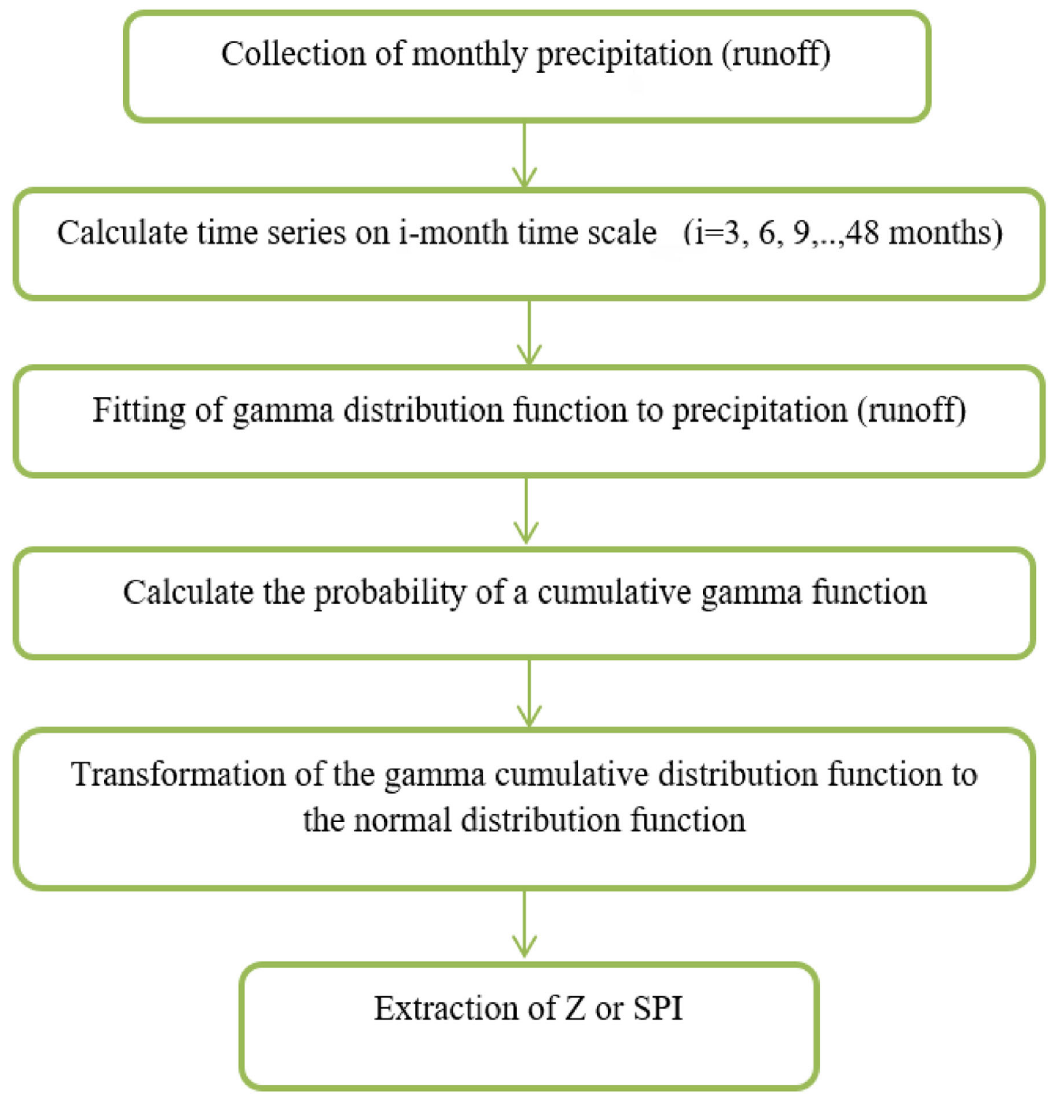
2.2. Standardized Precipitation (Runoff) Index

As mentioned above, to study meteorological drought, several indicators have been developed, of which the standardized precipitation index (SPI), first developed by McKee et al. [8], is particularly widely used. For hydrological drought, an index similar to the SPI can be developed as the standardized runoff index (SRI), which is based on monthly mean streamflow and was first proposed by Shukla and Wood [16]. The computational principles of these indices are presented in Figure 2. To forecast the SPI and SRI indices, the commonly known ARIMA model was used [25]. All steps of stochastic modeling were performed in R software in version 4.1.2.

When the time series is stationary, the basic form of ARMA models for a standardized normal variable Z_t can be used [32]:

$$Z_t={{\displaystyle \sum }}_{i=1}^p{\phi }_i{Z}_{i-1}-{{\displaystyle \sum }}_{j=1}^q{\mathsf{\theta }}_j{\epsilon }_{t-j} \mathrm{for} {\mathsf{\theta }}_0=-1,$$

(1)

where Z_t is the observed series, φ is the polynomial of order p, and θ is the polynomial of order q.

If a time series is nonstationary, it can be made stationary using the difference operator. Using the dth difference of the time series and modeling it with ARMA (p,q) leads to the emergence of a new set of nonseasonal autocorrelated cumulative moving average models (ARIMA (p,d,q)). The basic form of the nonseasonal ARIMA model follows [32]:

$$\phi \left(B\right){\left(1-B\right)}^d{Z}_t=\mathsf{\theta }\left(B\right){\epsilon }_t,$$

(2)

where φ and θ are polynomials of order p and q, respectively, and B is the lag operator that returns previous values of Z_t.

$$\phi \left(B\right)=\left(1-{\phi }_{1}B-{\phi }_2{B}^2-\cdots -{\phi }_p{B}^p\right),$$

(3)

$$\mathsf{\theta }\left(B\right)=\left(1-{\mathsf{\theta }}_{1}B-{\mathsf{\theta }}_2{B}^2-\cdots -{\mathsf{\theta }}_q{B}^q\right),$$

(4)

In the case of using the seasonal difference operator with delay w and their fitting with ARMA models (p, q), ARIMA seasonal models (P, D, Q)_w are created. A combination of seasonal and nonseasonal models forms the so-called multiplicative ARIMA models. The basic form of this model follows [33]:

$${\mathsf{\Phi }}_P\left(B^w\right){\phi }_p\left(B\right){\left(1-B^w\right)}^D{\left(1-B\right)}^d{Z}_t={\mathsf{\Theta }}_Q\left(B^w\right){\mathsf{\theta }}_q\left(B\right){\epsilon }_t,$$

(5)

where p is the order of the nonseasonal AR model, P is the order of the seasonal AR model, q is the order of the nonseasonal MA model, Q is the order of the seasonal MA model, w is the season length, ε is a random variable (net perturbation), and B is the lag operator B(Z_t) = Z_t−1, (1 − B)^d is equal to d of the second nonseasonal difference and (1 − B^w)^D is equal to D of the second seasonal difference of size w [33].

The development of time series models includes three stages: identification, parameter estimation, and a model adequacy test [17]. In the identification step, the general form of the model is determined according to the time series behavior. In the parameter estimation stage, the parameters of the model selected in the previous stage are calculated by a statistical method such as the momentum method or least squares and maximum likelihood. Finally, in the model adequacy test stage or diagnostic check, the selected model is used to model the time series and criteria such as the normality test and the independence of the residual are measured.

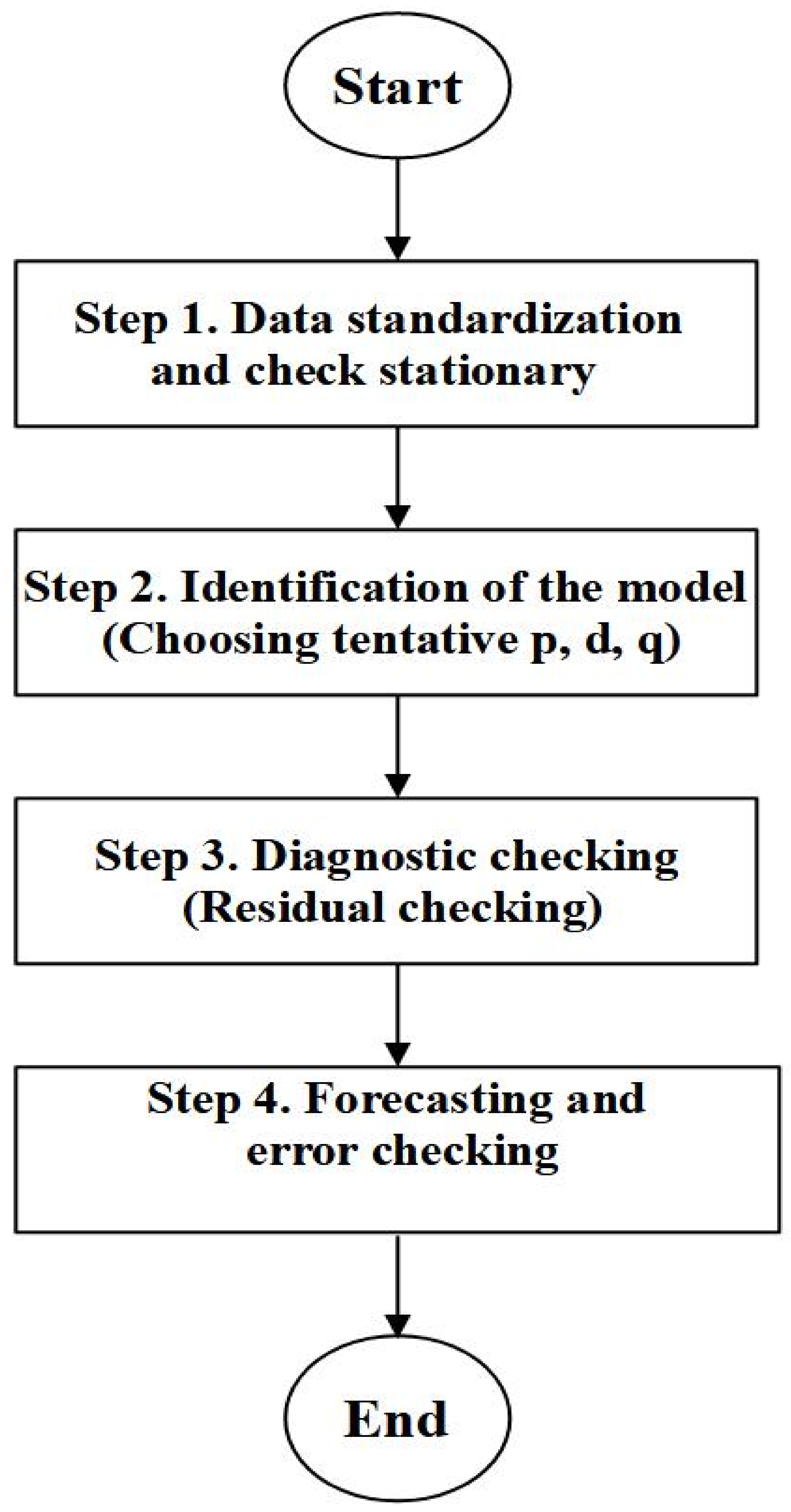
2.3. Model Development

The first step is the model identification. At this stage, the time series correlation structure is determined by testing the autocorrelation function (ACF) and partial autocorrelation (PACF) [17]; this information is then used to determine the general form of the univariate model. According to the number of significant steps in each of the ACF and PACF diagrams, the range of order changes of the models can be obtained. Finally, by combining them, the candidate models can be found. The model with the lowest Akaike information criterion (AIC) and Schwarz Bayesian criterion (SBC) is selected as the best model. The mathematical formulas of AIC [34] and SBC [35] follow:

$$AIC=N·ln\left({\sigma }_{\epsilon }^2\right)+2\left(m\right),$$

(6)

$$SBC=-2log\left(L\right)+\left(m\right)ln\left(n\right),$$

(7)

where m = (p + q + P + Q) is the number of estimated parameters and L is the likelihood function of ARIMA models.

After the model identification step, the parameters of each selected model were calculated. Preliminary estimates of the parameters were calculated from the ACF time series obtained at the identification stage.

The parameter estimation is followed by the diagnostic check. In this step, first the residual series is obtained from the difference of the observed time series and the model-predicted time series fit, then two validation tests are performed on the residues: (i) the white noise ACF and PACF of residuals and (ii) the normal probability of residuals and Kolmogorov–Smirnov statistics of residuals. Concerning the first test, if the ACF and PACF values of the residual series are consistent with zero within the confidence range, there is no significant correlation between the residues, and the residues are pure perturbation [18]. With respect to the latter test, the Kolmogorov–Smirnov (K–S) statistic is used to test the normality of residuals from different sets of models of the fit of data, as follows:

$$D=max\left|F\left(x\right)-\stackrel{}{F}\left(x\right)\right|,$$

(8)

where D is the maximum deviation, $F\left(x\right)$ is the completely specified theoretical cumulative distribution function under the null hypothesis, and $\stackrel{}{F}\left(x\right)$ is the sample cumulative density function based on n observations. For a chosen significance level α, if D is greater than the critical value D_tab, the null hypothesis related to normality is rejected for the chosen level of significance.

2.4. Kappa (κ)

Comparing the SPI (SRI) classes in the observed and predicted series, the disagreement between the mild drought and the moderate drought categories is not as great as the disagreement between the mild drought and the severe drought categories. Therefore, by considering certain weights for each case of disagreement, it is possible to make a more accurate comparison of the classes in the observed and predicted series. In this paper, we used kappa statistics [36,37,38] to comparison observed and predicted series.

The significant test statistic of the weighted kappa, statistic with the null disagreement hypothesis is as follows [37]:

$$t=\frac{\kappa }{\sqrt{\frac{\sum w_{\mathit{ij}}^2{p}_{e,\mathit{ij}}-{\left(\sum w_{\mathit{ij}}{p}_{e,\mathit{ij}}\right)}^2}{n}}}$$

(9)

where n is the number of series observations.

2.5. Model Validation

To evaluate the accuracy of the hydrological and meteorological drought forecasts and forecasting performance of models at the validation stage, results were compared based on the correlation coefficient (R²), Mean Absolute Error (MAE), and Root Mean Square Error (RMSE) [20,39].

$$R^2=\frac{{{\displaystyle \sum }}_{t=1}^n\left(x_t-{\overline{x}}_t\right)\left({\acute{x}}_t-{\overline{\acute{x}}}_t\right)}{\sqrt{{{\displaystyle \sum }}_{t=1}^n}}$$

(10)

$$\mathrm{RMSE}=\sqrt{\frac{{{\displaystyle \sum }}_{i=1}^n{\left(O_i-E_i\right)}^2}{n}},$$

(11)

$$\mathrm{MAE}=\frac{{{\displaystyle \sum }}_{j=1}^n\left|O_i-E_i\right|}{n},$$

(12)

Figure 3 shows a flowchart of the proposed method for drought forecasting. All modeling steps were performed using R software, version 4.1.2.

3. Results

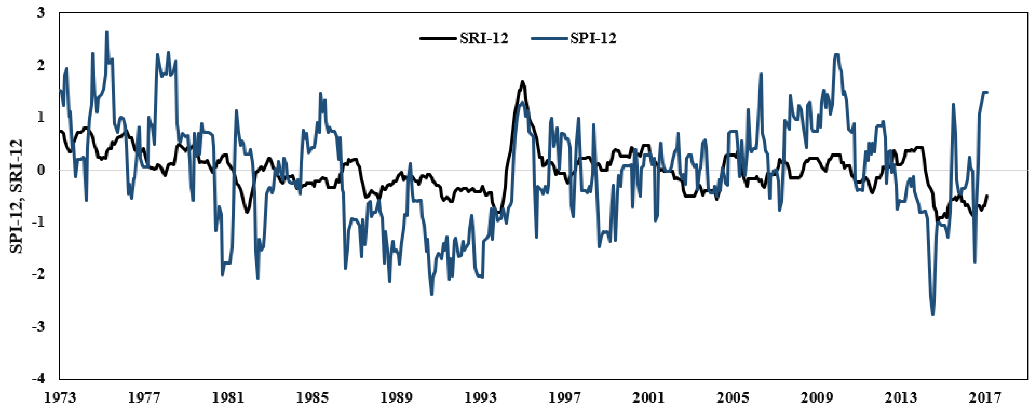
3.1. Assessment of Drought Based on SPI and SRI

In this study, SPI and SRI time series on a 12-month time scale were calculated using monthly precipitation and runoff data over a 45-year period (1973–2017). A 12-month duration of drought is one of the most common among other time scales in the studied watershed [40,41]. Moreover, in larger catchments, there is a strong relationship between meteorological and hydrological droughts if analyses are conducted for a more extended accumulation period [42,43].

According to Li et al. [44], the SPI is highly sensitive to onset of meteorological droughts, because meteorological droughts usually occur after the continuous lack of precipitation, but the SRI is effective in identifying the duration and termination of drought. Figure 4 shows the changes of SPI-12 and SRI-12 in the study area. The two variables follow an almost similar trend, and runoff and precipitation show a severe drought in the late 1980s and early 1990s, and generally dry conditions since the late 1990s. Time lags appear between SPI and SRI due to the delayed response of runoff to precipitation variability [45]. It can be therefore be observed that the time of the onset of hydrological drought tends to be later than the meteorological drought in most of the drought events. According to Sattar and Kim [46], the onset time of hydrological drought lags behind meteorological drought. This situation is similar to the one presented in this study. Data from 1973 to 2010 were used for model development and 2011 to 2017 for validation, and the three modeling steps were performed on each series.

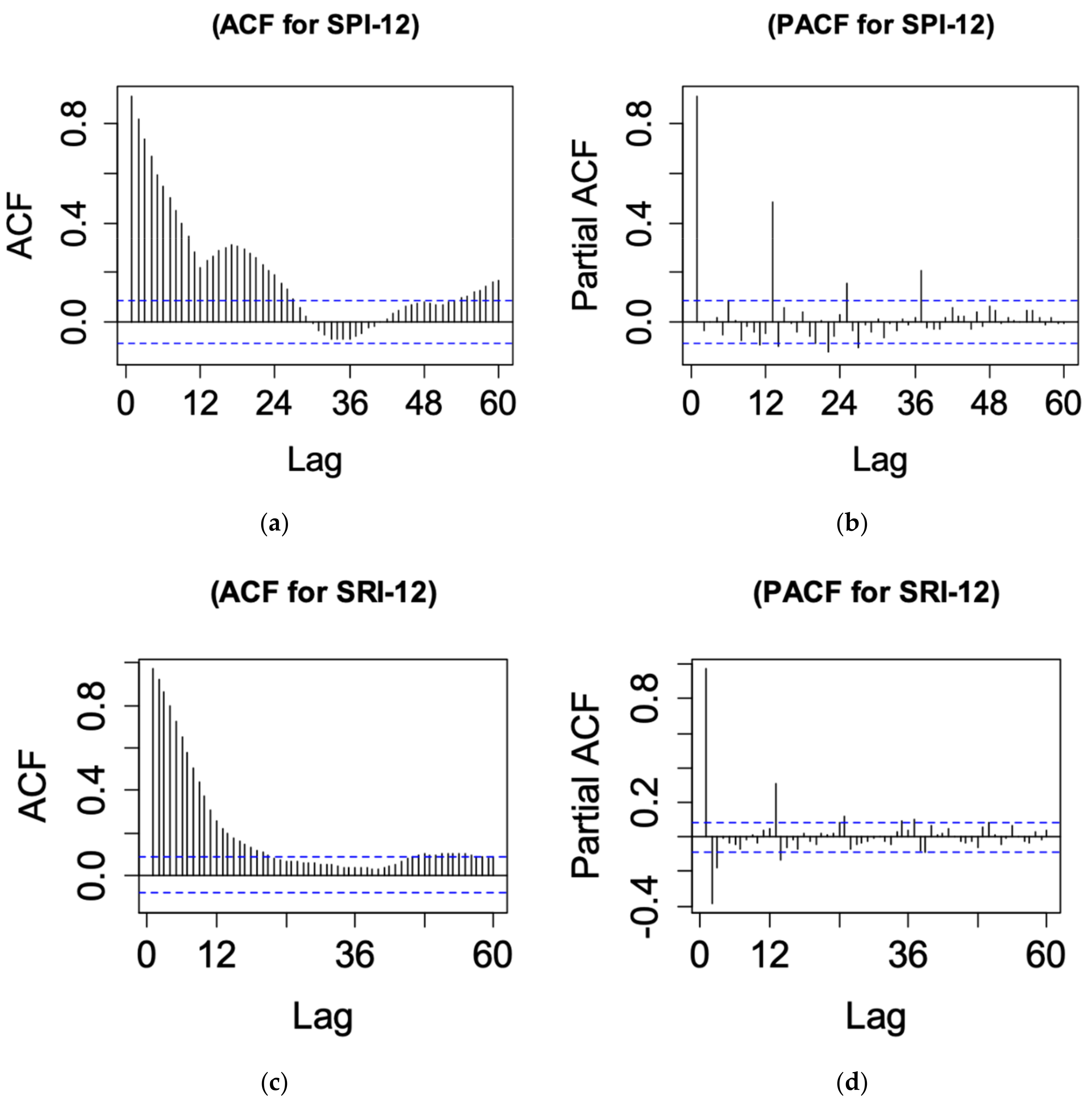
3.2. Stochastic Model Development

Figure 5 shows the ACF and PACF correlograms of the SPI-12 and SRI-12 time series. Owing to the ACF fluctuations in SPI-12 (Figure 5a), the time series is a combination of exponential and sinusoidal damping waves, and lagged correlations are significant in the first 20 time steps. Therefore, an MA model can be proposed. In the case of its PACF (Figure 5b), it is significant in the first step, which can suggest an AR model. In addition, the PACF is significant at 12 and 24 months, so the series has a 12-month period indicative of an annual cycle in precipitation. Therefore, a combination of AR and MA models as a multiplicative SARIMA model is proposed for modeling this series. The same applies to the SRI-12. ACF (Figure 5c) is attenuated as a combination of exponential and sinusoidal waves, and in the first 10 time steps, it is significant that an MA model with different orders can be proposed, and PACF (Figure 5d) in steps 1, 2, and 3 means that an AR model can be proposed with degrees 0, 1, 2, and 3. It also has a periodicity of 12 and 24, which indicates that the model is seasonal. Therefore, this variable is also a multiple (seasonal) ARIMA model.

According to the number of significant steps in each of the ACF and PACF diagrams, the range of order changes of the models can be obtained and finally, by combining them, the candidate models can be obtained. A model with the least AIC and SBC is selected as the best model. All SPI-12 and SRI-12 time series models were identified and the best model for each time series based on AIC and SBC was obtained from more than 860 candidate models. The same model was selected as the best by Han et al. [47] to drought forecasting in the Guanzhong Plain.

Table 2. Summary of AIC and BIC parameters of the best-fitted ARIMA models.

Index	Model	AIC	BIC
SPI-12	ARIMA(0,1,0)(0,1,1)12	605.25	613.74
	ARIMA(0,1,1)(0,0,1)12	321.57	334.38
	ARIMA(1,0,1)(1,1,0)12	754.55	771.54
	ARIMA(1,0,1)(0,1,1)12	587.61	604.61
	ARIMA(1,0,0)(2,0,1)12	320.11	345.74
SRI-12	ARIMA(1,0,1)(1,0,0)12	−1277.37	−1255.90
	ARIMA(2,0,0)(2,0,0)12	−1355.60	−1329.84
	ARIMA(2,0,1)(1,0,0)12	−1305.33	−1279.57
	ARIMA(2,1,0)(2,0,0)12	−1360.34	−1338.88
	ARIMA(2,1,2)(1,0,1)12	−1481.87	−1451.83

shows an example of several models, parameters, and criteria of AIC and BIC. The standard error calculated for each of the model parameters was generally small compared to the parameters. Therefore, these parameters can be used in modeling.

Then, validation tests were performed on the residues to evaluate the adequacy of the selected model, which are ACF and PACF residuals and residual histogram and normal residual probability. Figure 6a,b shows ACF and PACF residues for SPI-12 time series and Figure 6c,d shows SRI-12 for two selected ARIMA models (0,1,0)(0,1,1)₁₂ and ARIMA (2,0,1)(1,0,1)₁₂, respectively. According to the figures, it can be seen that most of the ACF and PACF values in both indices are within the confidence limit. Therefore, there is no significant correlation between the residuals; the residuals are white noise.

Figure 7 shows the residual histogram and the normal probability for the SPI-12 and SRI-12 time series. According to Figure 7a,b, it can be seen that the residuals of both time series follow the normal distribution, so the residuals are white noise and the cumulative distribution plot of the residuals is a straight line when drawn on normal probabilistic paper. Therefore, the residuals follow the normal distribution.

3.3. Drought Forecasting Using Selected Models

For validation, the time series from 2011 to 2017 was used for SPI-12 and SRI-12. In Figure 8a,b, comparison of the observed and predicted time series shows the two drought indicators. As the results show, there is good agreement between the two series. That is, the time series model was able to simulate drought indices well.

The main statistical features were compared between the observed and predicted data using Z test for mean and F test for standard deviation. The results are presented in

Table 3. Summary of the statistical analysis of model parameters.

Index		Variables in the Model
	Model	Parameter	Value of Parameters	Standard Error	t-Ratio	p
SPI	ARIMA (0,1,0)(0,1,1)12	Θ1	−1.00	0.02	−57.66	0
	ARIMA(0,1,1)(0,0,1)12	θ1	−0.01	0.04	−0.29	0.77
		Θ1	−0.71	0.03	−24.54	0
	ARIMA(1,0,1)(1,1,0)12	ϕ1	0.87	0.02	34.87	0
		θ1	0.11	0.05	2.09	0.04
		Φ1	−0.71	0.03	−22.22	0
	ARIMA(1,0,1)(0,1,1)12	ϕ1	0.91	0.02	45.49	0
		θ1	0.01	0.05	0.25	0.81
		Θ1	−1.00	0.02	−53.63	0
	ARIMA(1,0,0)(2,0,1)12	ϕ1	0.98	0.01	121.44	0
		Φ1	−0.15	0.08	−1.93	0.05
		Φ2	−0.01	0.06	−0.23	0.82
		Θ1	−0.62	0.07	−9.21	0
SRI	ARIMA(1,0,1)(1,0,1)12	ϕ1	0.98	0.01	118.45	0
		θ1	0.35	0.03	10.22	0
		Φ1	−0.46	0.04	−11.66	0
	ARIMA(2,0,0)(2,0,0)12	ϕ1	1.42	0.04	36.79	0
		ϕ2	−0.44	0.04	−11.22	0
		Φ1	−0.59	0.04	−13.88	0
		Φ2	−0.29	0.04	−6.82	0
	ARIMA(1,0,1)(1,0,0)12	ϕ1	1.37	0.11	12.91	0
		θ1	0.08	0.1	0.77	0.44
		Φ1	−0.47	0.04	−12.03	0
	ARIMA(2,1,0)(2,0,0)12	ϕ1	0.38	0.04	8.83	0
		ϕ2	0.12	0.04	2.69	0.01
		Φ1	−0.59	0.04	−13.98	0
		Φ2	−0.30	0.04	−7.13	0
	ARIMA(2,1,2)(1,0,1)12	ϕ1	−0.06	0.36	−0.18	0.86
		ϕ2	0.45	0.26	1.74	0.08
		θ1	0.45	0.36	1.25	0.21
		θ2	−0.14	0.15	−0.93	0.35
		Φ1	0.05	0.05	0.99	0.32
		Θ1	−0.95	0.03	−36.98	0

Note: Bold and underline indicates the best model.

.

The results of the mean test (Z test) indicate that the null hypothesis, that the means are equal, is accepted for the time series SPI-12 and SRI-12 at a significance level of 95%; therefore, the stochastic model maintains the observed series average well. The results of the variance comparison test (F test) indicate that the null hypothesis, that the variances are equal, is accepted at the 95% significance level for the time series studied. Therefore, there is no significant difference between the observed and predicted values of variance.

We also calculated weighted kappa in drought classes. Based on the results shown in

Table 4. Comparison of statistical properties of the observed and predicted data in model validation.

Index	SPI	SRI
Model	ARIMA (1,0,1)(0,1,1)12	ARIMA (1,0,1)(1,0,1)12
Kw	0.79	0.88
Variance (Observed)	0.97	0.17
Variance (Forecasted)	0.81	0.16
F test	1.12	1.06
Mean (Observed)	−0.187	−0.263
Mean (Forecasted)	−0.174	−0.26
Z	−0.013	−0.012
RMSE	0.46	0.067
MAE	0.02	−0.002
R	0.89	0.98

, there is good agreement between observed in drought classes and predicted (K > 0.7).

The forecast was performed for SPI-12 and SRI-12 from 1 to 12 month lead times using the best model.

Table 5. Coefficient of correlation, RMSE, and MAE between observed and predicted data for lead time 1 to 12.

Lead Time	SPI-12			SRI-12
	R2	RMSE	MAE	R2	RMSE	MAE
1	0.96	0.43	−0.026	0.97	0.061	−0.001
2	0.9	0.45	−0.028	0.966	0.06	−0.016
3	0.87	0.55	−0.049	0.961	0.058	−0.018
4	0.86	0.58	−0.054	0.96	0.11	0.03
5	0.85	0.64	−0.089	0.95	0.14	0.07
6	0.8	0.67	−0.001	0.92	0.17	0.09
7	0.78	0.78	−0.012	0.91	0.19	0.1
8	0.71	0.84	−0.022	0.88	0.23	0.12
9	0.68	0.89	−0.033	0.86	0.28	0.15
10	0.65	0.91	−0.052	0.84	0.29	0.16
11	0.58	0.93	−0.080	0.74	0.37	0.19
12	0.51	0.98	−0.091	0.7	0.39	0.21

shows R², RMSE, and MAE values between observed data and predicted data using the selected best model for all time series. Results show that with a longer lead time, the coefficient of correlation decreases and error coefficient increases between observed and predicted data. The best models selected from the multiplicative ARIMA approach using a time series data of SPI-12 and SRI-12 series can be used for drought forecasting at whatever lag is desired.

4. Discussion

Generally, the results show that SPI and SRI indicators have a similar behavior and SRI tends to occur later than SPI indicators for particular events. In this study, the ARIMA model was used to forecast meteorological and hydrological drought. The popularity of the ARIMA model in many areas is due to its flexibility and the systematic searching at each stage (identification, estimation, and diagnostic check) for an appropriate model [18]. Quite visible differences in the behavior of ACF and PACF between SPI and SRI can be explained by mechanisms influencing the two forms of drought.

Comparison of multiplicative SARIMA models used in meteorological and hydrological droughts shows that increasing the forecast lead time (from 1 to 12 months) increases the error rate. The reason for this is the cumulative error from the previous steps, which spreads to the next steps [21]. It can be concluded that stochastic models provide good results in the case study only for the next 12 months; in other words, it is better to use this linear statistical approach to forecast only the next 12 monthly steps ahead to prevent anomalies in the results, and for more than 12 months to consider using other models.

Meteorological drought in this region is determined by a high variability of precipitation and is influenced by the El Niño Southern Oscillation (ENSO) [48], Mediterranean Oscillation (MO) [49], and Western Mediterranean Oscillation (WeMO) [50,51]. The negative phase of the NAO dominated between 1940 and 1980, corresponding to a period when precipitation was above normal and thus SPI generally had positive values in the Mediterranean basin [52]. More recently, drier conditions dominated, corresponding to commonly negative SPI values (Figure 4). These teleconnections with climate indices offer additional possibilities for drought forecasting approaches.

Considering the hydrological drought, expressed by SRI, a lag time between the occurrence of meteorological and hydrological drought is visible. It is mainly visible in Figure 8, where negative SRI are observed after negative SPI. The time buffering is influenced by catchment properties, including land cover, geological properties, and human activities. The ARIMA model (1,0,1) (0,0,1) for the SPI and (1,0,1) (1,0,1) for the SRI model were found as the best models to predict drought. Moreover, the models help to identify seasonality of SPI and SRI indicators that is strongly dependent on the precipitation seasonal variability.

The ARIMA model has some limitation, as it is not suitable for nonlinear relationships, especially in a complex and dynamic problems [53], and is incapable of fully capturing nonlinear patterns hidden within a time series. These limitations are less of a problem for forecasting SPI and SRI, which are transformed to follow a standard normal distribution, as compared to precipitation and streamflow, whose distribution is highly non-normal.

Our results are broadly consistent with those of studies from other regions of the world that tried to use the ARIMA model to predict meteorological and hydrological drought. Karimi et al. [54] detected that an ARIMA model can be used to forecast SPI index in 1, 3, 6, 9, 12 monthly time scales in the Karkheh River watershed. Han et al. [47] describe results of drought forecasting where the ARIMA model linked with remote sensing was used to analyze change of the Vegetation Temperature Condition Index (VTCI) in the Guanzhong Plain. Finally, they conclude that the ARIMA model gave accurate results in forecasting the index. In contrast, Beyaztas and Yaseen [55] showed that Functional Principal Component Analysis (FPCA) gave better results compared to the ARIMA model when predicting the Palmer Drought Severity Index (PDSI).

5. Conclusions

Drought forecasting is an important issue, especially in arid regions and under climate change. Many techniques are used to forecast drought, but one of the more popular is the ARIMA model. In this work, a multiplicative ARIMA model was used for meteorological and hydrological drought forecast in the Wadi Ouaharane watershed located in Algeria. Moreover, the model can be used in other regions and different types of catchments because parameters of the ARIMA model are optimized based on time series. The model does not have parameters that are linked with catchment features; instead, the model only requires time series characteristics. To use the ARIMA model, a long time series with constant time steps is necessary.

Drought was indicated by the SPI representing meteorological drought and the SRI for hydrological drought. Results showed that despite some similarity between the courses of the two indices, time lags appear between SPI and SRI due to the delayed response of runoff to precipitation variability. Analyses showed that the ARIMA model (1,0,1) (0,0,1) for the SPI and (1,0,1) (1,0,1) for the SRI were found as the best models to predict drought. Based on R², both models had good quality; for the SPI and the SRI, R² was equal to 0.96 and 0.97, respectively, at 1-month lag. Finally, we conclude that the seasonal ARIMA model can be used to forecast meteorological and hydrological drought indices in arid regions.

References

1. Tsakiris, G.; Pangalou, D.; Vangelis, H. Regional drought assessment based on the Reconnaissance Drought Index (RDI). Water Res. Manag. 2007, 21, 821–833. [Google Scholar] [CrossRef]
2. Tsakiris, G.; Vangelis, H. Establishing a drought index incorporating evapotranspiration. Eur. Water 2005, 9–10, 3–11. [Google Scholar]
3. Mishra, A.K.; Singh, V.P. A review of drought concepts. J. Hydrol. 2010, 391, 202–216. [Google Scholar] [CrossRef]
4. Boken, V.K.; Cracknell, A.P.; Heathcote, R.L. Monitoring and Predicting Agricultural Drought: A Global Study; Oxford University Press: Oxford, UK, 2005. [Google Scholar]
5. Wilhite, D.A.; Svoboda, M.D.; Hayes, M.J. Understanding the complex impacts of drought: A key to enhancing drought mitigation and preparedness. Water Resour. Manag. 2007, 21, 763–774. [Google Scholar] [CrossRef] [Green Version]
6. Wilhite, D. A methodology for drought preparedness. Nat. Hazards 1996, 13, 229–252. [Google Scholar] [CrossRef] [Green Version]
7. Palmer, W.C. Meteorlogical Drought; Research Paper No. 45; US Department of Commerce Weather Bureau: Washington, DC, USA, 1965; pp. 1–58.
8. McKee, T.B.; Doesken, N.J.; Kleist, J. The relationship of drought frequency and duration to time scales. In Proceedings of the 8th Conference on Applied Climatology, Anaheim, CA, USA, 17–22 January 1993; pp. 179–184. [Google Scholar]
9. Bera, B.; Shit, P.K.; Sengupta, N.; Saha, S.; Bhattacharjee, S. Trends and variability of drought in the extended part of Chhota Nagpur plateau (Singbhum Protocontinent), India applying SPI and SPEI indices. Environ. Chall. 2021, 5, 100310. [Google Scholar] [CrossRef]
10. Stagge, J.H.; Kingston, D.G.; Tallaksen, L.M.; Hannah, D.M. Observed drought indices show increasing divergence across Europe. Sci. Rep. 2017, 7, 14045. [Google Scholar] [CrossRef]
11. Dukat, P.; Bednorz, E.; Ziembińska, K.; Urbaniak, M. Trends in drought occurrence and severity at mid-latitude European stations (1951–2015) estimated using standardized precipitation (SPI) and precipitation and evapotranspiration (SPEI) indices. Meteorol. Atmos. Phys. 2022, 134, 20. [Google Scholar] [CrossRef]
12. Guttman, N.B. Comparing the Palmer drought severity index and the standardized precipitation Index. J. Am. Water Res. Assoc. 1998, 34, 113–121. [Google Scholar] [CrossRef]
13. Caloiero, T. Drought analysis in New Zealand using the standardized precipitation index. Environ. Earth Sci. 2017, 76, 569. [Google Scholar] [CrossRef]
14. Hayes, M.J.; Svoboda, M.; Wilhite, D.A.; Vanyarkho, O. Monitoring the 1996 drought using the SPI. Bull. Am. Meteorol. Soc. 1999, 80, 429–438. [Google Scholar] [CrossRef] [Green Version]
15. Paulo, A.A.; Pereira, L.S. Drought concepts and characterization: Comparing drought indices applied at local and regional scales. Water Int. 2006, 31, 37–49. [Google Scholar] [CrossRef]
16. Shukla, S.; Wood, A.W. Use of a standardized runoff index for characterizing hydrologic drought. Geophys. Res. Lett. 2008, 35, 226–236. [Google Scholar] [CrossRef] [Green Version]
17. Box, G.E.P.; Jenkins, G.M. Time Series Analysis: Forecasting and Control, 1st ed.; Holden-Day: San Francisco, CA, USA, 1970. [Google Scholar]
18. Zhang, G.P. Time series forecasting using a hybrid ARIMA and neural network model. Neurocomputing 2003, 50, 159–175. [Google Scholar] [CrossRef]
19. Hu, W.; Tong, S.; Mengersen, K.; Connell, D. Weather variability and the incidence of cryptosporidiosis: Comparison of time series Poisson regression and SARIMA models. Ann. Epidemiol. 2007, 17, 679–688. [Google Scholar] [CrossRef]
20. Modarres, R. Streamflow drought time series forecasting. Stoch. Environ. Res. Risk Assess. 2007, 21, 223–233. [Google Scholar] [CrossRef]
21. Mishra, A.; Desai, V. Drought Forecasting Using Stochastic Models. Stoch. Environ. Res. Risk Assess. 2005, 19, 326–339. [Google Scholar] [CrossRef]
22. Fernandez, C.; Vega, J.A.; Fonturbel, T.; Jimenez, E. Streamflow drought time series forecasting: A case study in a small watershed in North West Spain. Stoch. Environ. Res. Risk Assess. 2009, 23, 1063–1070. [Google Scholar] [CrossRef]
23. Durdu, O.F. Application of Linear Stochastic Models for Drought Forecasting in the Buyuk Menderes River Basin, Western Turkey. Stoch. Environ. Res. Risk Assess. 2010, 24, 1145–1162. [Google Scholar] [CrossRef]
24. Bazrafshan, O.; Salajegheh, A.; Bazrafshan, J.; Mahdavi, M.; Maraj, A.F. Hydrological drought forecasting using ARIMA models (case study: Karkheh Basin). Ecopersia 2015, 3, 1099–1117. [Google Scholar]
25. Al Sayah, M.J.; Abdallah, C.A.; Khouri, M.; Darwich, T. A framework for climate change assessment in Mediterranean data-sparse watersheds using remote sensing and ARIMA modeling. Theor. Appl. Climatol. 2021, 143, 639–658. [Google Scholar] [CrossRef]
26. Shatanawi, K.; Bahbeh, M.; Shatanawi, M. Characterizing, Monitoring and Forecasting of Drought in Jordan River Basin. J. Water Resour. Prot. 2013, 5, 12. [Google Scholar] [CrossRef] [Green Version]
27. Buttafuoco, G.; Caloiero, T. Drought events at different timescales in southern Italy (Calabria). J. Maps 2014, 10, 529–537. [Google Scholar] [CrossRef]
28. Caloiero, T.; Veltri, S. Drought assessment in the Sardinia region (Italy) during 1922–2011 using the standardized precipitation index. Pure Appl. Geophys. 2019, 176, 925–935. [Google Scholar] [CrossRef]
29. Zhu, B.; Chevallier, J. Carbon Price Forecasting with a Hybrid ARIMA and Least Squares Support Vector Machines Methodology. In Pricing and Forecasting Carbon Markets; Springer: Berlin/Heidelberg, Germany, 2017. [Google Scholar]
30. Benkhaled, A.; Remini, B. Variabilité temporelle de la concentration en sédiments et phénomène d’hystérésis dans le bassin de l’Oued Wahrane (Algérie). Hydrol. Sci. J. 2003, 48, 243–255. [Google Scholar] [CrossRef] [Green Version]
31. Köppen, W. Das Geographische System der Klimate. Handbuch der Klimatologie; Köppen, W., Geiger, R., Eds.; Verlag von Gebrüder Borntraeger: Berlin, Germany, 1936; Volume 1, pp. 1–44. [Google Scholar]
32. Mikosch, T.; Gadrich, T.; Klüppelberg, C.; Adler, R.J. Parameter Estimation for ARMA Models with Infinite Variance Innovations. Ann. Stat. 1995, 23, 305–326. [Google Scholar] [CrossRef]
33. Yevjevich, V. An Objective Approach to Definitions and Investigations of Continental Hydrologic Droughts; Colorado State University: Fort Collins, CO, USA, 1967. [Google Scholar]
34. Akaike, H. On the likelihood of a time series model. J. R. Stat. Soc. Ser. D 1978, 27, 217–235. [Google Scholar] [CrossRef]
35. Schwarz, G. Estimating the dimension of a model. Ann. Stat. 1978, 6, 461–464. [Google Scholar] [CrossRef]
36. Cohen, J. Weighted kappa: Nominal scale agreement provision for scaled disagreement or partial credit. Psychol. Bull. 1968, 70, 213. [Google Scholar] [CrossRef]
37. Kumar, M.N.; Murthy, C.S.; Sai, M.V.R.S.; Roy, P.S. On the use of Standardized Precipitation Index (SPI) for drought intensity assessment. Meteorol. Appl. 2009, 16, 381–389. [Google Scholar] [CrossRef] [Green Version]
38. Landis, J.R.; Koch, G.G. An Application of Hierarchical Kappa-type Statistics in the Assessment of Majority Agreement among Multiple Observers. Biometrics 1977, 33, 363. [Google Scholar] [CrossRef] [PubMed]
39. Roughani, M.; Ghafouri, M.; Tabatabaei, M. An innovative methodology for the prioritization of sub-catchments for flood control. Int. J. Appl. Earth Obs. Geoinf. 2007, 9, 79–87. [Google Scholar] [CrossRef]
40. Pińskwar, I.; Choryński, A.; Kundzewicz, Z.W. Severe Drought in the Spring of 2020 in Poland—More of the Same? Agronomy 2020, 10, 1646. [Google Scholar] [CrossRef]
41. Młyński, D.; Wałega, A.; Kuriqi, A. Influence of meteorological drought on environmental flows in mountain catchments. Ecol. Indic. 2021, 133, 108460. [Google Scholar] [CrossRef]
42. Tokarczyk, T.; Szalińska, W. Drought hazard assessment in the process of drought risk management. Acta Sci. Pol. Form. Circumiectus 2018, 18, 217–229. [Google Scholar] [CrossRef]
43. Kubiak-Wójcicka, K.; Pilarska, A.; Kamiński, D. The Analysis of Long-Term Trends in the Meteorological and Hydrological Drought Occurrences Using Non-Parametric Methods—Case Study of the Catchment of the Upper Noteć River (Central Poland). Atmosphere 2021, 12, 1098. [Google Scholar] [CrossRef]
44. Li, Y.; Gong, Y.; Huang, C. Construction of combined drought index based on bivariate joint distribution. Alex. Eng. J. 2021, 60, 2825–2833. [Google Scholar] [CrossRef]
45. Niu, J.; Chen, J.; Sun, L.Q. Exploration of drought evolution using numerical simulations over the Xijiang (West River) basin in South China. J. Hydrol. 2015, 526, 68–77. [Google Scholar] [CrossRef]
46. Sattar, M.N.; Kim, T.W. Probabilistic characteristics of lag time between meteorological and hydrological droughts using a Bayesian model. Terr. Atmos. Ocean. Sci. 2018, 29, 709–720. [Google Scholar] [CrossRef] [Green Version]
47. Han, P.; Wang, P.X.; Zhang, S.Y.; Zhu, D.H. Drought forecasting based on the remote sensing data using ARIMA models. Math. Comput. Model. 2010, 51, 1398–1403. [Google Scholar] [CrossRef]
48. Lloyd-Huhes, B.; Saunders, M.A. A drought climatology for Europe. Int. J. Climatol. 2002, 22, 1571–1592. [Google Scholar] [CrossRef]
49. Conte, M.; Giuffrida, A.; Tedesco, S. The Mediterranean Oscillation. Impact on Precipitation and Hydrology in Italy Climate Water; Publications of the Academy of Finland: Helsinki, Finland, 1989. [Google Scholar]
50. Muthoni, F.K.; Odongo, V.O.; Ochieng, J.; Mugalavai, E.M.; Mourice, S.K.; Hoesche-Zeledon, I.; Mwila, M.; Bekunda, M. Long-term spatial-temporal trends and variability of precipitation over Eastern and Southern Africa. Theor. Appl. Climatol. 2019, 137, 1869–1882. [Google Scholar] [CrossRef] [Green Version]
51. Martín-Vide, J.; López-Bustins, J.A. The Western Mediterranean Oscillation and Precipitation in the Iberian Peninsula. Int. J. Climatol. 2006, 26, 1455–1475. [Google Scholar] [CrossRef]
52. Kelley, C.; Ting, M.; Seager, R.; Kushnir, Y. Mediterranean precipitation climatology, seasonal cycle, and trend as simulated by CMIP5. Geophys. Res. Lett. 2012, 39, L21703. [Google Scholar] [CrossRef] [Green Version]
53. Papastefanopoulos, V.; Linardatos, P.; Kotsiantis, S. COVID-19: A Comparison of Time Series Methods to Forecast Percentage of Active Cases per Population. Appl. Sci. 2020, 10, 3880. [Google Scholar] [CrossRef]
54. Karimi, M.; Meleese, A.M.; Khosravi, M.; Mamuye, M.; Zhang, J. Chapter 26—Analysis and prediction of meteorological drought using SPI index and ARIMA model in the Karkheh River Basin Iran. In Extreme Hydrology and Climate Variability; Melesse, A.M., Abtew, W., Senay, G., Eds.; Elsevier: Amsterdam, The Netherlands, 2019; pp. 343–353. [Google Scholar] [CrossRef]
55. Beyaztas, U.; Yaseen, Z.M. Drought interval simulation using functional data analysis. J. Hydrol. 2019, 579, 124141. [Google Scholar] [CrossRef]
Figure 1. Location, topographic characteristics, pluviometric, and hydrometric network of the study area.
Climate 10 00036 g001
Figure 2. Methodology of SPI and SRI.
Climate 10 00036 g002
Figure 3. Model development in stochastic models.
Climate 10 00036 g003
Figure 4. The SPI-12 and SRI-12 time series plot for the Wadi Ouahrane basin.
Climate 10 00036 g004
Figure 5. ACF and PACF correlograms and 95% confidence limits for stochastic monthly series for the Wadi Ouahrane basin (ad).
Climate 10 00036 g005
Figure 6. Diagnostic check of the best-fitted multiplicative ARIMA model for SPI-12 (a,b) and SRI-12 (c,d) time series for the Wadi Ouahrane watershed.
Climate 10 00036 g006
Figure 7. Normal probability plot and residual histogram for SPI-12 (a) and SRI-12 (b).
Climate 10 00036 g007
Figure 8. Comparison of SPI-12 (a) and SRI-12 (b) series observed and predicted in the validation phase for 1-month lead time.
Climate 10 00036 g008