
Data-Driven Diagnosis of PV-Connected Batteries: Analysis of Two Years of Observed Irradiance


1
Hawaiʻi Natural Energy Institute, University of Hawaiʻi at Mānoa, 1680 East West Road, POST 109, Honolulu, HI 96822, USA
2
Computer Science Department, Polytechnic School of Engineering, University of Oviedo, 33202 Gijon, Spain
3
University of Hawai’i at Mānoa, 2500 Campus Road, Honolulu, HI 96822, USA
*
Author to whom correspondence should be addressed.
Batteries 2023, 9(8), 395; https://doi.org/10.3390/batteries9080395
Submission received: 27 June 2023
/
Revised: 11 July 2023
/
Accepted: 25 July 2023
/
Published: 29 July 2023
(This article belongs to the Special Issue The Precise Battery—towards Digital Twins for Advanced Batteries)
Abstract
:The diagnosis and prognosis of PV-connected batteries are complicated because cells might never experience controlled conditions during operation as both the charge and discharge duty cycles are sporadic. This work presents the application of a new methodology that enables diagnosis without the need for any maintenance cycle. It uses a 1-dimensional convolutional neural network trained on the output from a clear sky irradiance model and validated on the observed irradiances for 720 days of synthetic battery data generated from pyranometer irradiance observations. The analysis was performed from three angles: the impact of sky conditions, degradation composition, and degradation extent. Our results indicate that for days with over 50% clear sky or with an average irradiance over 650 W/m2, diagnosis with an average RMSE of 1.75% is obtainable independent of the composition of the degradation and of its extent.

1. Introduction
Photovoltaic (PV) technology has been rapidly developing in the past two decades, and it is predicted that more than 324 GW of new solar capacity will be added to the grid in the United States in the next decade, quadrupling current levels [1]. Storage will help reduce the impact of intermittency and increase grid benefits. Electrochemical storage will consist of both grid-scale and smaller residential storage [1,2].
To ensure maximum performance and optimal safety, batteries require regular assessments of their state of health (SOH). However, assessing SOH for operational PV-tied systems is problematic due to the sporadic nature of charge and discharge. In recent years, there has been a tremendous effort towards the development of new methodologies for SOH estimation [3,4], with a lot of novelty coming from the emergence of data-driven approaches [5,6,7,8,9] as pioneered by Severson et al. [10]. Unfortunately, many studies suffer from a lack of data that prevents the extension of the results outside of the tested conditions. While online databases [11,12,13] can remediate this issue to some extent, the data is often not varied enough to represent the sporadic conditions cells will experience in deployed systems [14]. This lack of diversity can be alleviated by supplementing experimental data with synthetic data and leveraging the benefits of transfer learning [15]. Besides physic-based models [16,17,18,19,20,21], the other main modeling approach considered for generating synthetic data is the mechanistic approach [22,23,24]. Because this approach simulates the impact of degradation modes [24,25] rather than trying to replicate every possible degradation, it offers fast simulations with high fidelity, making it an excellent candidate to simulate a large number of data samples. The benefits of using this approach for synthetic data were previously demonstrated [26], and such datasets were applied to the training of different machine learning algorithms in recent years [14,27,28,29,30,31,32]. The main drawback of most current synthetic datasets when deployed systems are considered is that they provide low-rate constant current data, which is typically not available in real applications without performing lengthy maintenance cycles. This limitation has been circumvented with the latest version of our mechanistic modeling framework, which enables simulations outside of constant current [33]. This new feature has been used in our previous work [34], where we proposed a new methodology for diagnosis that used real observed solar irradiance, modeled clear sky irradiance, and synthetically generated battery data from a digital twin. The approach was demonstrated to be effective for the opportunistic diagnosis of PV-connected batteries without the need for any maintenance cycles. Our results showed that diagnosis of was possible if clear-sky conditions occurred for at least half of the day. However, significant performance variations were observed for skies with similar cloud coverage, which indicated that the tested sample (18 days) was too small to get a full understanding of the approach’s applicability. To remediate this issue, this follow-up work tested the approach’s validity on a newly generated dataset consisting of the 720 days of our observed irradiance dataset from Maui, HI, USA.
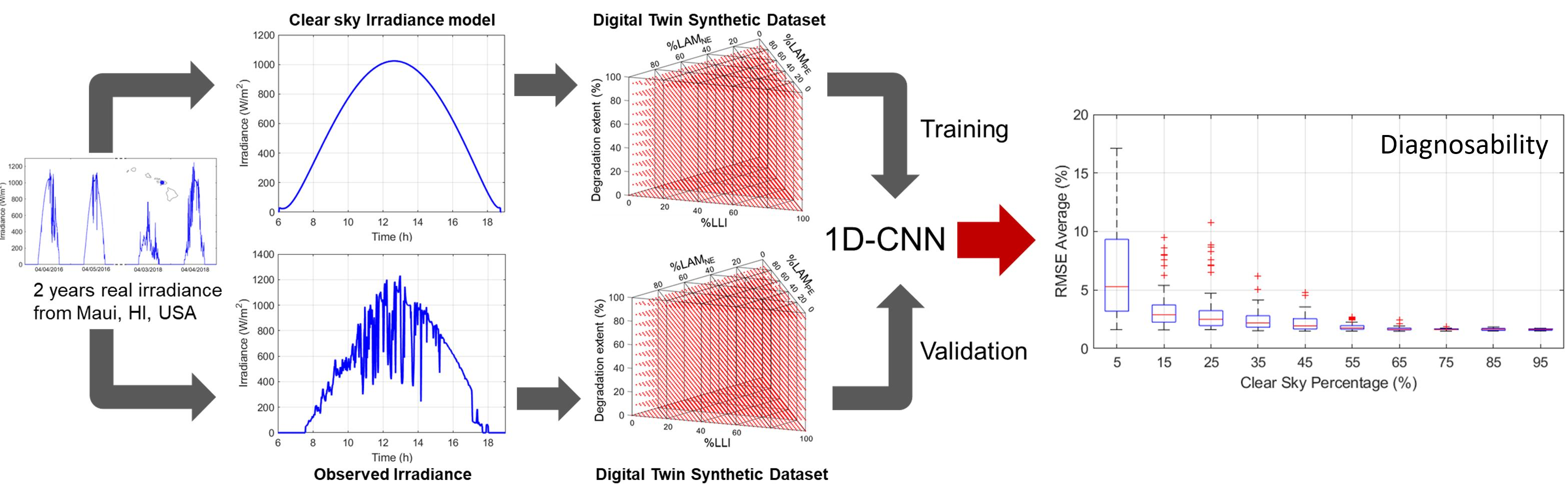
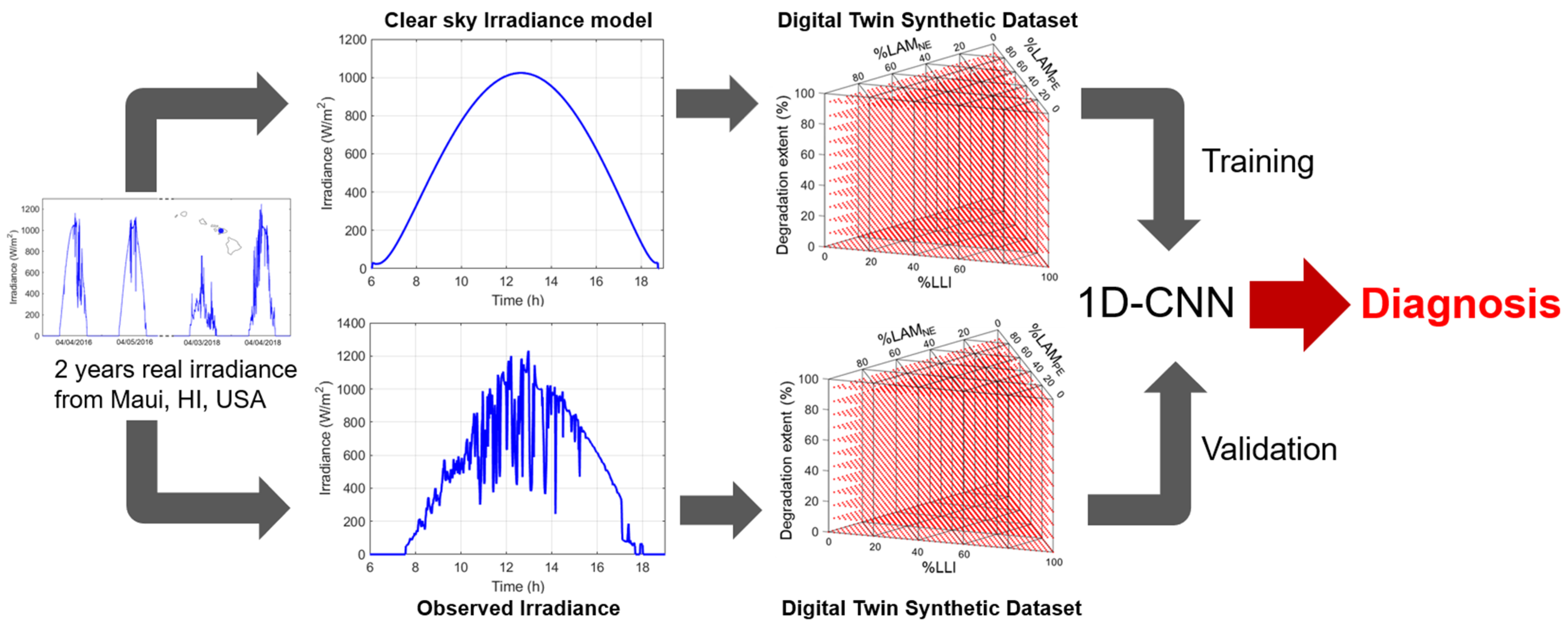
The overall approach for this work is summarized in Figure 1. For the 720 days tested period, the voltage response was simulated using output from a clear-sky irradiance model in conjunction with nearly 45,000 different degradations for the battery [34]. This synthetic dataset was then used to train a 1D convolutional neural network (CNN) to enable the quantification of battery degradation. The algorithm, developed by Kim et al. [28], was selected from our previous work [34], where it offered the best compromise between accuracy and calculation time compared to other tested algorithms. A second synthetic dataset was generated using the same methodology but using the observed irradiance data instead of the modeled one for every day of the dataset. The resulting data was filtered with the help of two metrics: the clear sky percentage (cs%) [34] and the average daily irradiance (|Irr|). In addition, the diagnosis accuracy was evaluated from three different angles: the sky conditions for which this diagnosis is more accurate, the degradation paths for which the opportunistic diagnosis is more favorable, and the extent of degradation for which the diagnosis could be considered valid. The diagnosis accuracies obtained from the analysis of 10,000 degradations for 720 days allowed for a better understanding of the potential of using synthetic data generated from clear sky irradiances for opportunistic diagnosis of deployed PV-connected batteries.
2. Materials and Methods
The irradiance dataset used in this work contains observations collected over a two-year period from a PV test site located at the Maui Economic Development Board office on the southwestern coast of the island of Maui, Hawaiʻi, USA. The test site included instrumentation for high-frequency PV and solar resource monitoring, including a Kipp and Zonen SMP21-A secondary pyranometer mounted in the plane of array (POA) of installed PV systems. The data was collected at 1 Hz and averaged over 1 min for data collection.
As in [34], a clear sky irradiance model (CSM) was used. It was based on the model proposed by Ineichen and Perez [35] for a horizontal surface but included modifications to estimate clear sky irradiance on a tilted surface by recomputing the solar angle of incidence, adding a reduction of diffuse irradiance received [36], and adding a ground reflected irradiance source [37]. In order to determine if an irradiance observation was occurring under a clear sky, its value was compared to the output from the CSM. This information was then used to calculate the cs%.
The battery digital twin comprised HNEI’s ‘alawa mechanistic battery model [24,33] and half-cell data harvested from a commercial cell with a graphite (G) negative electrode (NE) and a Nickel Manganese Cobalt oxide (NMC) positive electrode (NE) with a 1:1:1 stoichiometry. The model parameterization at different rates was detailed in [34], and the parameters are provided in Appendix B. As proposed in [33], and to handle the non-constant current duty cycles, calculations were undertaken at 150 different rates to be able to select the most adapted voltage/rate couple matching the power request for each point of duty cycle [34]. To avoid any overfitting error, each simulation was performed with parameters randomly varied by ±1% to be in the same range as observed cell-to-cell variations in commercial cells [38]. The synthetic data used in this work, both for training and testing, was generated using the method described in [14,26,27] by scanning the entire range of possible combinations for the thermodynamic degradation modes, the loss of lithium inventory (LLI), and the loss of active material (LAM) for the PE and NE up to 50% each. The resolution was set to 2.5% (861 unique triplets [LLI, LAMPE, LAMNE]) with 1% steps (50 simulations per triplet), resulting in around 45,000 unique degradations per simulation for the training and 5% (231 unique triplets and 11,000 degradations) for the testing [34].
The one-dimensional CNN [28] developed by Kim et al. was selected for this work due to its proven efficient quantification of degradation modes and because it offered the best compromise between accuracy and calculation cost [34]. The algorithm was trained, validated, and tested on both voltage vs. capacity and voltage vs. time curves since the duty cycles were not constant current. As explained in [34], the time (t)-based diagnosis would be preferable for deployed systems because it is directly measurable, but it was found more difficult to achieve than the capacity (Q)-based one. The model was implemented in TensorFlow [39] with 5 layers, of which 2 are CNN-1D layers with 32 neurons each and 3 are fully connected layers with 128, 64, and 3 neurons each. The batch size, learning rate, and number of epochs were fixed at 64, 0.001, and 25, respectively.
The statistical metrics used in this study are the root mean square error (RMSE), the mean absolute error (MAE), and the Pearson correlation coefficient (ρ), defined as follows:
With being the prediction, the prediction mean, the true value, the true mean, and the total number of data points.
For interested readers, more details on the experimental set up can be found in [34], of which this work is a direct follow-up using the exact same models and dataset.
3. Results
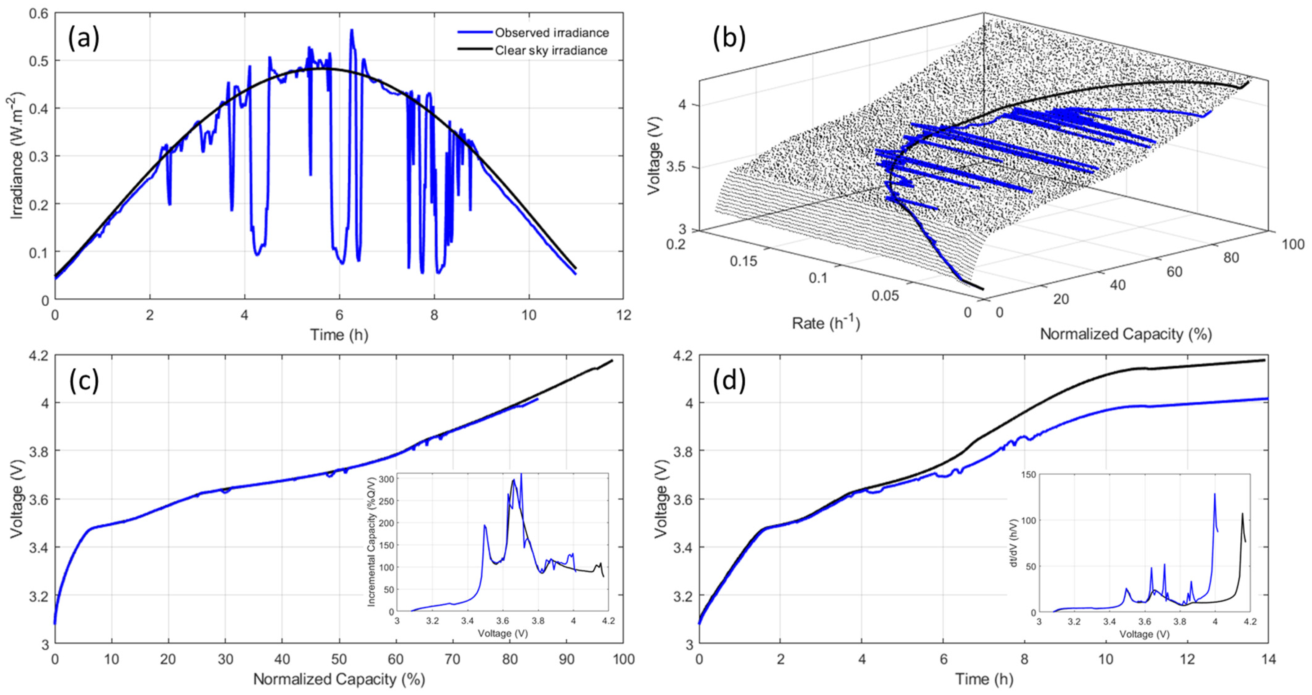
A sample day of input data is shown in Figure 2, with results for the observed irradiance in blue and the calculated clear sky one in black. Figure 2a showcases the irradiances where the effects of Intermittent cloud coverage can be seen, resulting in a cs% of 34 and a 15% reduction in |Irr| for the observed irradiance compared to the modeled one. Figure 2b presents the voltage response calculation process for duty cycles that are not constant currents. The thin black dotted curves represent 150 different simulations at constant current for rates evenly spread between C/100 and C/5. For each duty cycle and for each increment of capacity, the right couple voltage/rate were fetched to match the requested power (thick black and blue curves). For the observed irradiance duty cycle, and since there was less power generated because of the cloud coverage, the charge was incomplete, and the maximum capacity was not reached (thick black curve). Figure 2c displays the resulting voltage vs. capacity curves with the associated incremental capacity (IC) derivative as an inset. The drop in irradiance actually did not influence much the voltage vs. capacity curves, and despite the lower end-of charge voltage, the curves calculated from the observed and clear-sky irradiances are rather similar, with just a little noise visible between 30 and 70% normalized capacity. Looking at the incremental capacity curves allows for enhanced visualization of the differences, and it can be seen that, while the different features of the IC curves are not as well defined in the case of the data generated from the observed irradiance, the overall shape remained the same. The differences are more marked on the voltage vs. time curves (Figure 2d) because, while the low irradiance peaks will not charge much capacity, their duration is not negligible [34]. In this work, the process showcased in Figure 2b was repeated for more than 10,000 different degradation compositions where LLI and LAMs were each independently varied from 0 to 50% in 1% increments. The resulting data was used to train (clear sky data) and test (observed irradiance data) the algorithm.
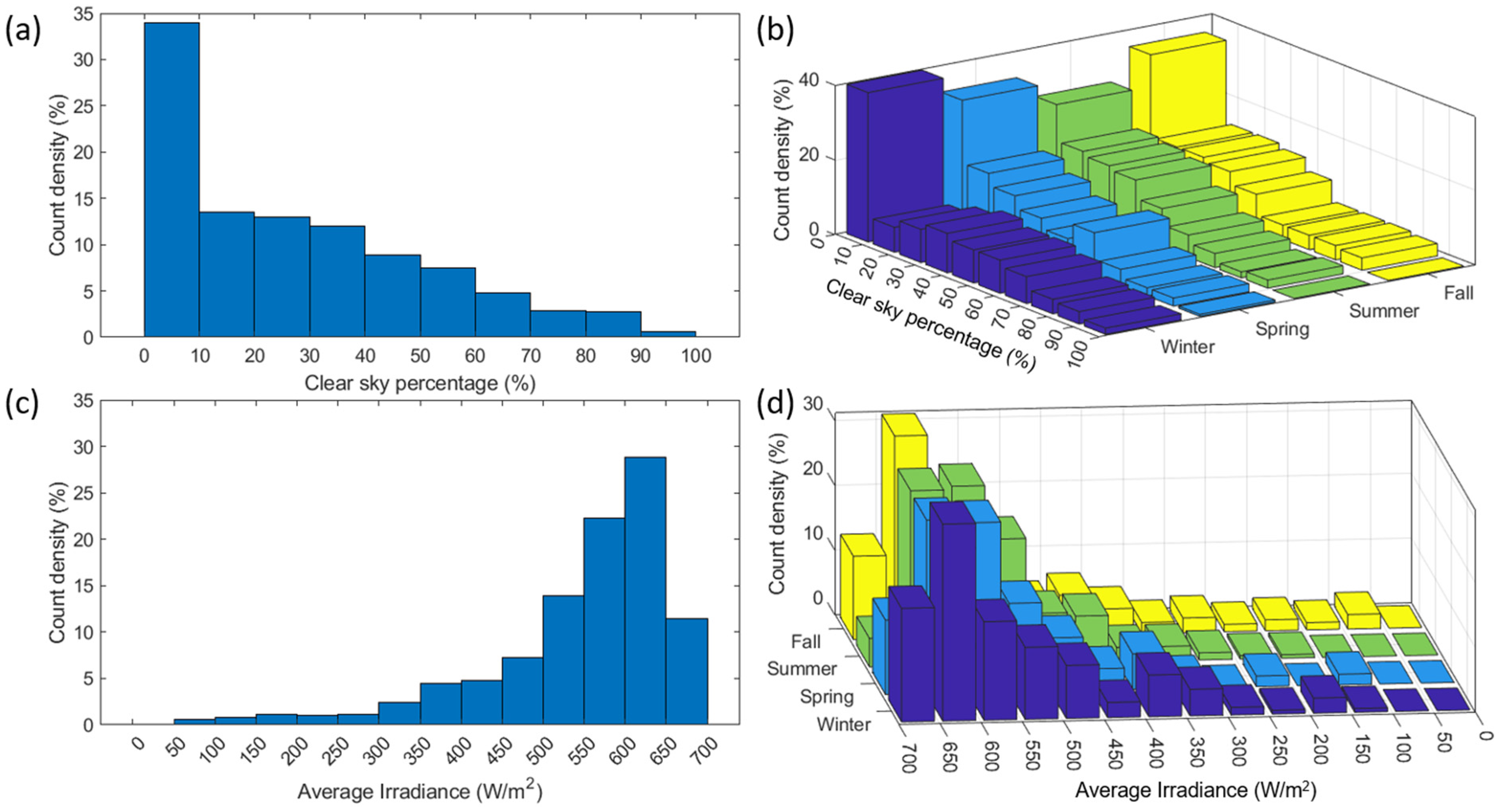
Before looking into the performance of the algorithm, Figure 3a,b present the distribution of the daily cs% observations in 10% increments for (a) the full 2-year period and (b) seasons. Overall, 34% of the 720 tested days had below 10% clear skies, with a peak in winter (40% of days) and a dip in summer (26% of days). This high percentage of days without a clear sky is not surprising given the tropical climate of the Hawaiian archipelago. From the results obtained in our previous work [34] on an 18 day sample, diagnosis seemed possible for days with 50% or more clear skies. This amounts to 20.5% of the 720 days in the dataset, with a maximum in winter (25%) and a minimum in summer (17.5%). In order to test if focusing on higher cs% improved diagnosis accuracy, the days for which the cs% is above 70% will also be studied in this work. This corresponds to 6% of days overall (9% winter, 4% summer). Since it was observed that the cs% might not be the only parameter to monitor to enable good diagnosis [34], this work also investigated the diagnosis accuracy as a function of the |Irr|, Figure 3c,d. Overall, |Irr| peaks on average around 625 W/m2 independently of the season. 75% of the days had an average irradiance above 500 W/m2 without much seasonal impact, whereas 40% of the days had an average irradiance above 600 W/m2 and 11.5% above 650 W/m2 (17.5% and 4.5% for winter and summer, respectively).
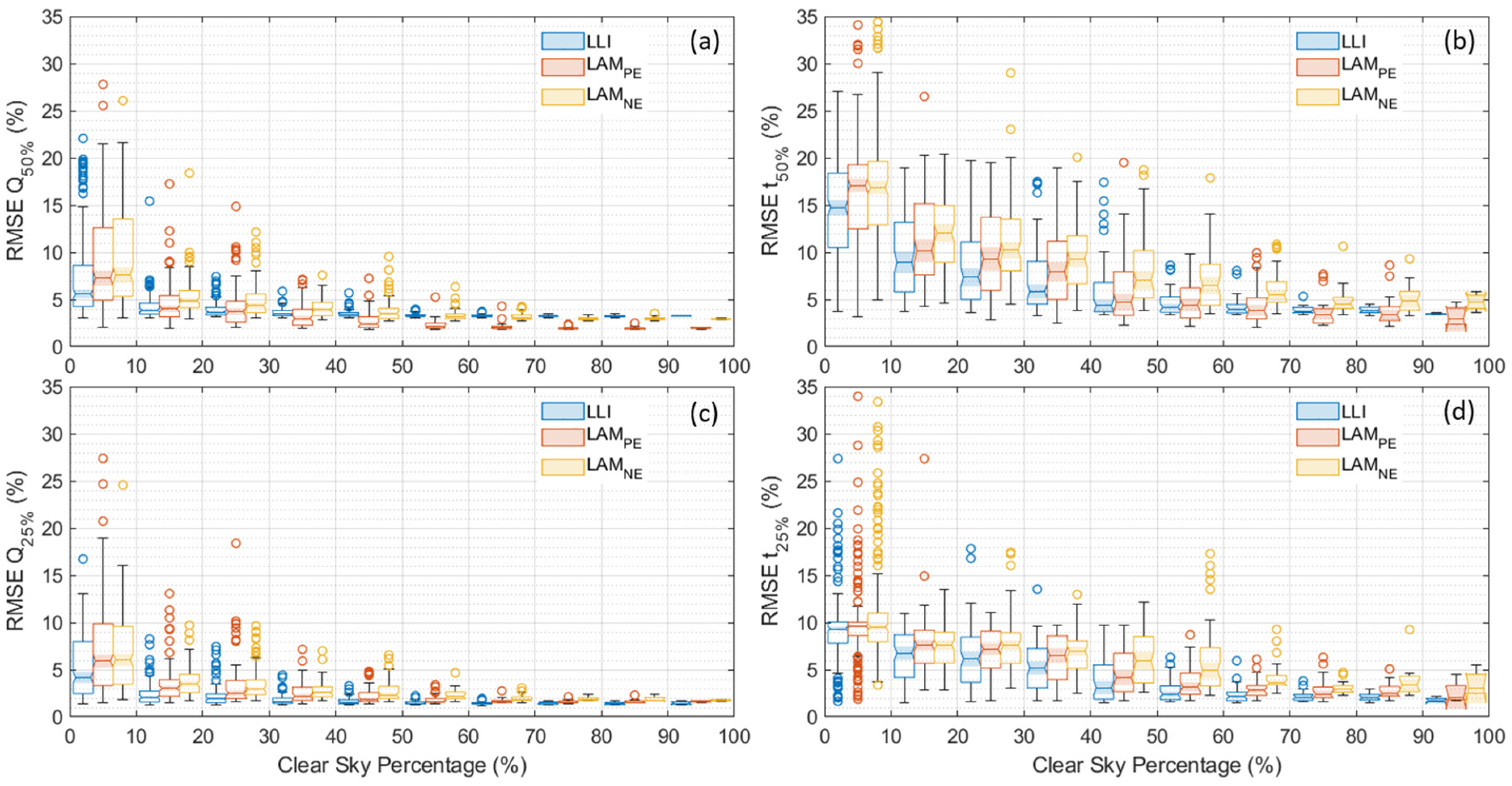
Figure 4 and Figure 5 present the evolution of the diagnosis RMSEs averaged for each 10% cs% and 50 W/m2 |Irr| increment, respectively. Results are plotted as box plots that display a summary of the diagnosis statistics with median, quartile, and outlier information. The box size corresponds to the interquartile range, i.e., the 50% of the data around the median. The line in the box is the median value, with the 95% confidence interval represented by the size of the notch and the filling. The whisker length corresponds to the distance to the last data point within 1.5 times the interquartile range. Values above or below the whiskers marked by circles are considered outliers. The four panels on the figures correspond to the distribution of the average RMSEs for (a) a Q-based diagnosis with degradation modes up to 50%, (b) the t-based diagnosis under the same conditions, (c) the Q-based diagnosis for up to 25% degradation, and (d) the t-based diagnosis under the same conditions. The three sets of results correspond to the individual degradation modes (LLI, LAMPE, and LAMNE, from left to right).
Looking at the evolution of the RMSEs with the cs% (Figure 4), it can be seen that they were on average 50% lower for the Q-based diagnosis compared to the t-based ones. This was reduced to 30% when the maximum degradation of 25% was used instead of 50%. This is similar to what was observed in [34] in the smaller sample. The distribution was also more monotonic than the one obtained with just 18 days [34], so the sample size increase did allow for stronger conclusions on the impact of cs%. The size of the interquartile range (i.e., the size of the box containing 50% of the data) was found to decrease with an increasing cs%. For the Q-based diagnosis, the RMSEs started to plateau around 50% cs% versus 70% for the t-based diagnosis. The bottom whiskers did seem to go down to their minimum for almost every cs% which indicates that cs% alone did not allow for all the days for which a good diagnosis is possible. However, with little to no outliers and a low RMSE at a high cs%, it is extremely efficient at selecting days with good opportunities for diagnosis. Finally, the RMSE for LLI estimation was most of the time lower than the one for LAMPE for low cs% but not necessarily for the higher ones. The LAMNE estimations were nearly always the ones with the worst RMSEs, except for high cs% when LAMPE’s were the worst.
Figure 5 presents similar data for |Irr| instead of cs%. In this case, there was a clear difference in minimum RMSE between the low and high averages, showcasing a better separation of the good and bad opportunities. For the Q-based diagnosis, the RMSEs started to plateau above 600 W/m2 while reaching their minimum above 650 W/m2 for both maximum degradations. For the t-based diagnosis, the plateau was not as marked, especially when higher degradations were considered (Figure 5b). It has to be noted that there were outliers even for the higher averages, which implies that |Irr| filtering did not guarantee a good diagnosis. In addition, the 95% confidence range for the medians drastically increased for the t-based diagnosis at low average irradiances compared to the Q-based ones.
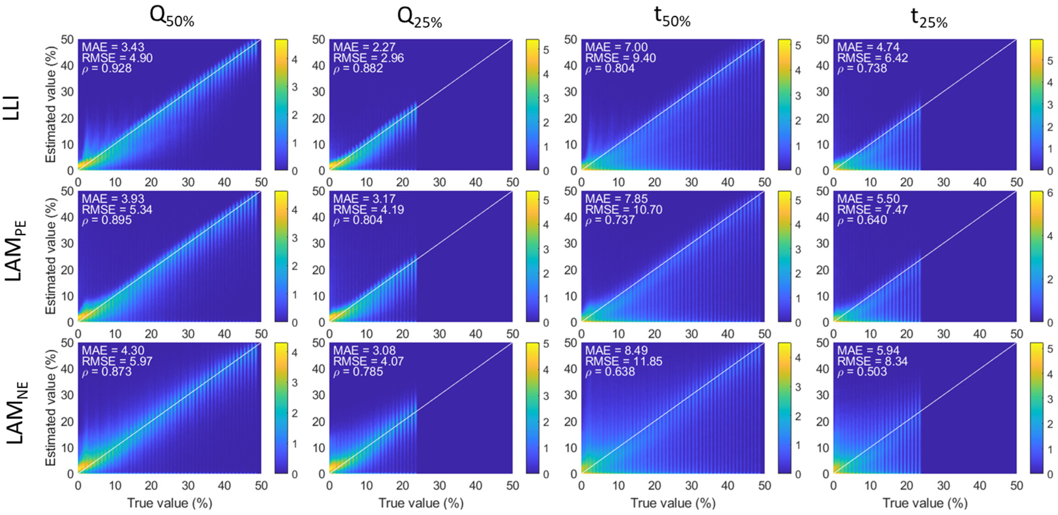
Table 1 presents a summary of the obtained statistical metrics for the five considered cases figure: the full dataset, over 50% and 70% cs%, and |Irr| over 600 and 650 W/m2. The best results were always obtained on days with over 70% cs%. In tied second came the over 50% cs% and over 650 W/m2 (1.13 times higher), with the over 50% being slightly better for the Q-based diagnosis versus the over 650 W/m2 being better for the t-based ones. Fourth came over 600 W/m2 (1.3 times higher), and, not surprisingly, the full dataset (2.4 times higher) came last. For all but the full dataset, the Q-based MAE were always around 2% up to 50% degradation and around 1.5% or below for 25% or less degradation. The values for t-based MAE were about twice as high as their Q-based counterparts. In addition, the correlation coefficients were all above 0.95 for the Q-based diagnoses and above 0.9 for the t-based ones, with only a few exceptions.
4. Discussion
The analysis of the results for the 10,000 degradations for the 720 days of the dataset confirmed that an accurate diagnosis for days with at most 50 cs% or an |irr| above 650 W/m2 is obtainable. This is especially true for the Q-based diagnosis, as the RMSEs were on average around 1.75% when considering up to 25% degradation. For the t-based diagnosis, the RMSEs were closer to 3.5% for the same conditions that account for more than one in five days in our dataset.
To complement this analysis, it is necessary to remember that these RMSE values are the average values obtained from 10,000 different degradation compositions, whose extent ranges from 1% to 50%. Therefore, it is possible that the overall average RMSE did not tell the full story and that it could have been influenced by compositions for which the method is not working or by their extent. In order to investigate this issue, the data was analyzed from two additional complementary angles: the impact of the degradation path and the impact of the degradation extent.
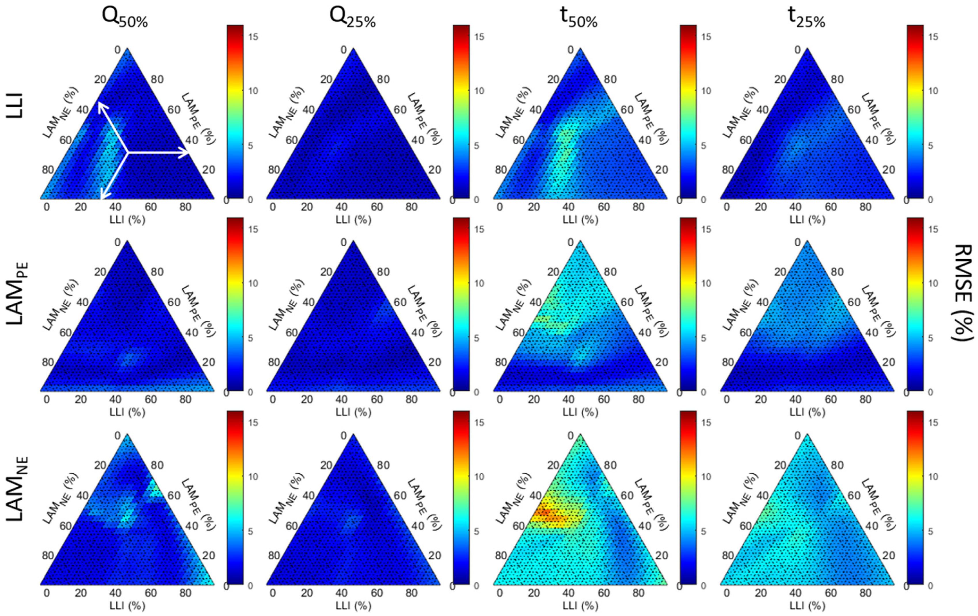
To investigate the impact of the degradation path, it is essential to first discuss the definitions of diagnosis and path dependence. Every battery degradation can be decomposed in terms of how much it affects the amount of lithium that can react, how much material is available to host it, and how fast that can be done. Every degradation can thus be summarized by the evolution of its degradation modes [24,25]. Excluding kinetic effects, every degradation has a unique composition of the three main degradation modes (LLI, LAMPE, and LAMNE). This composition will change depending on the battery usage; e.g., low temperatures might favor one over another, and the opposite might be true for high cut-off voltages. This is the path dependence of battery degradation. Since degradation can only be associated with a unique composition of the three main degradation modes, it can be represented on a ternary diagram (Figure 6). Every point in the triangle corresponds to a unique value of the [LLI, LAMPE, LAMNE] triplet, whose sum is always 1. The portion associated with each degradation mode can be found using the arrows in the top left panel, for which the current position indicates a 0.33:0.33:0.33 mix of the three degradation modes. This representation does not consider the extent of the degradation, as each point in the triangle is the average of all degradations for this composition (i.e., 1%:1%:1% to 50%:50%:50% for the 0.33:0.33:0.33 mix). To avoid confusion with the extent of the degradation, which will be discussed later, fractions will be used to describe the compositions.
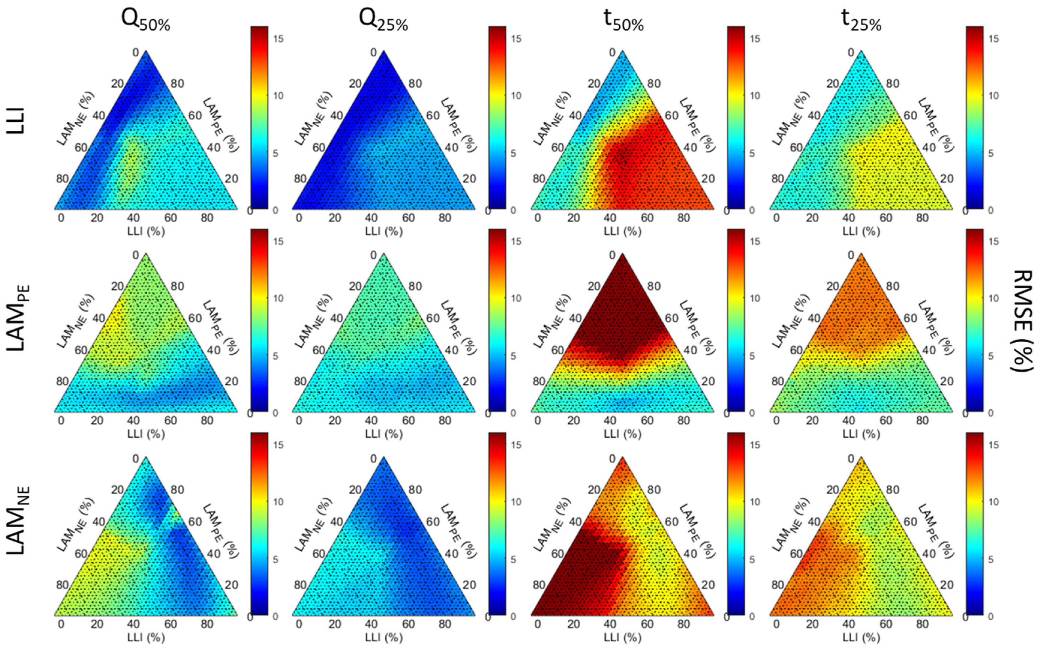
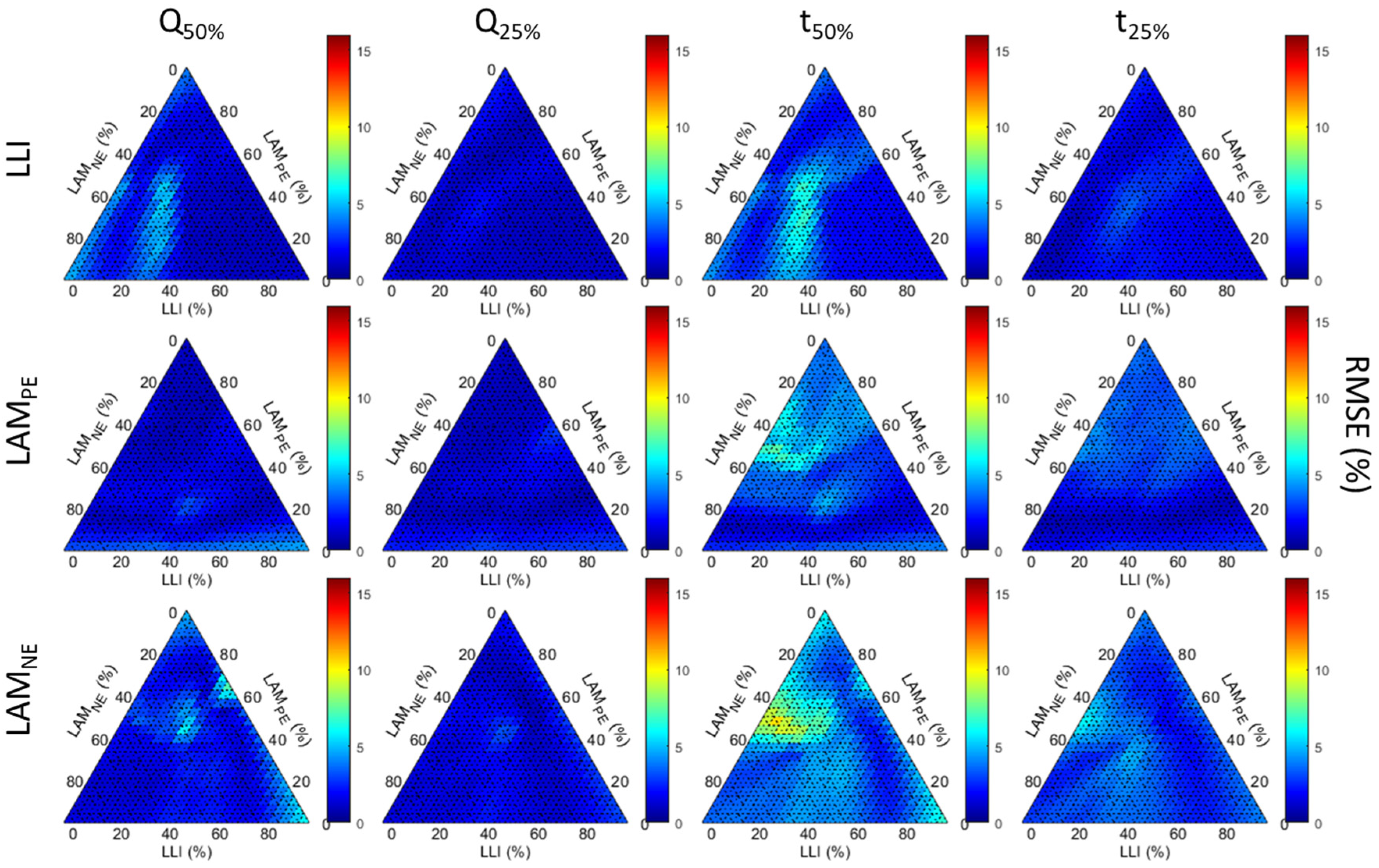
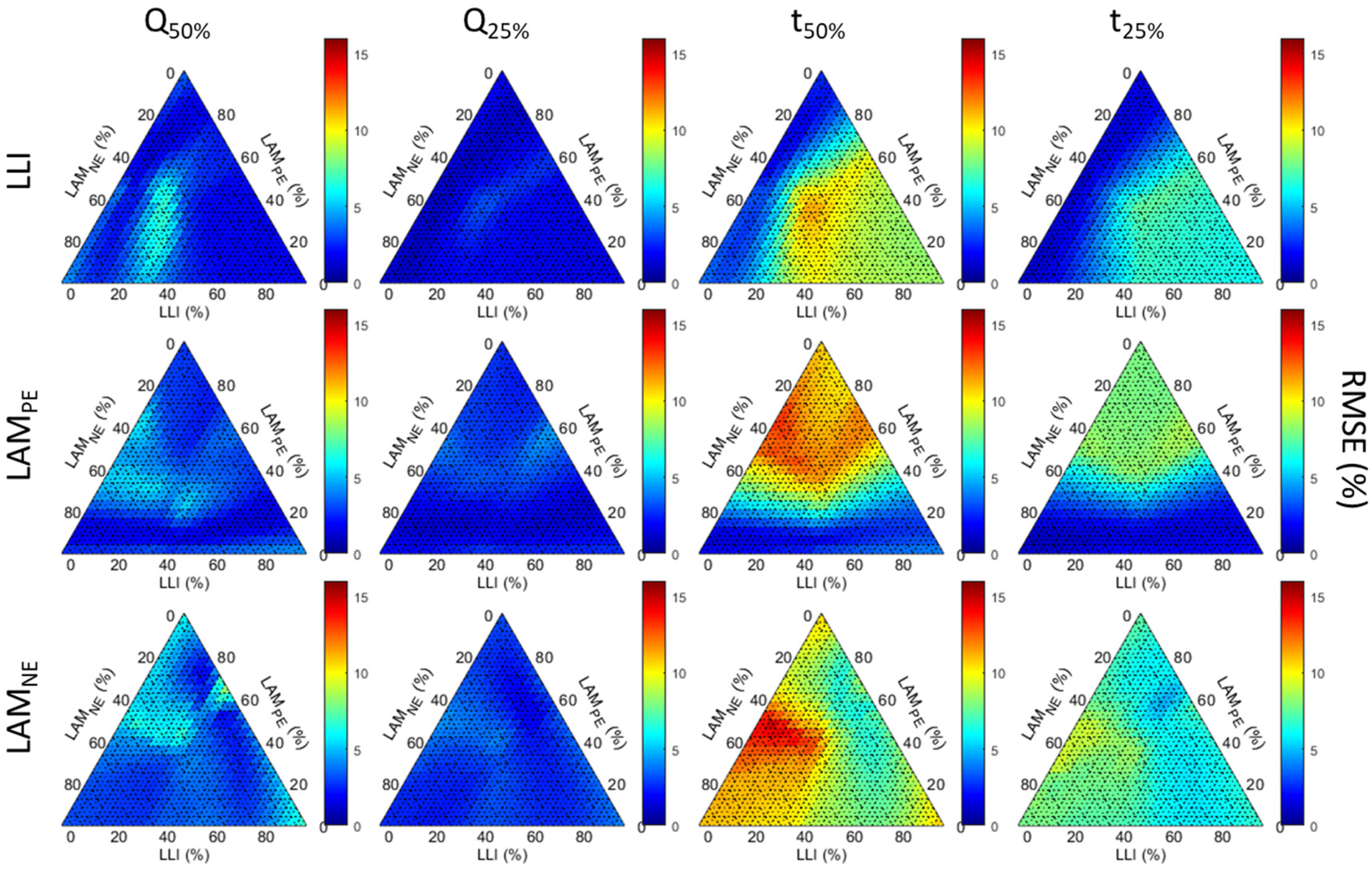
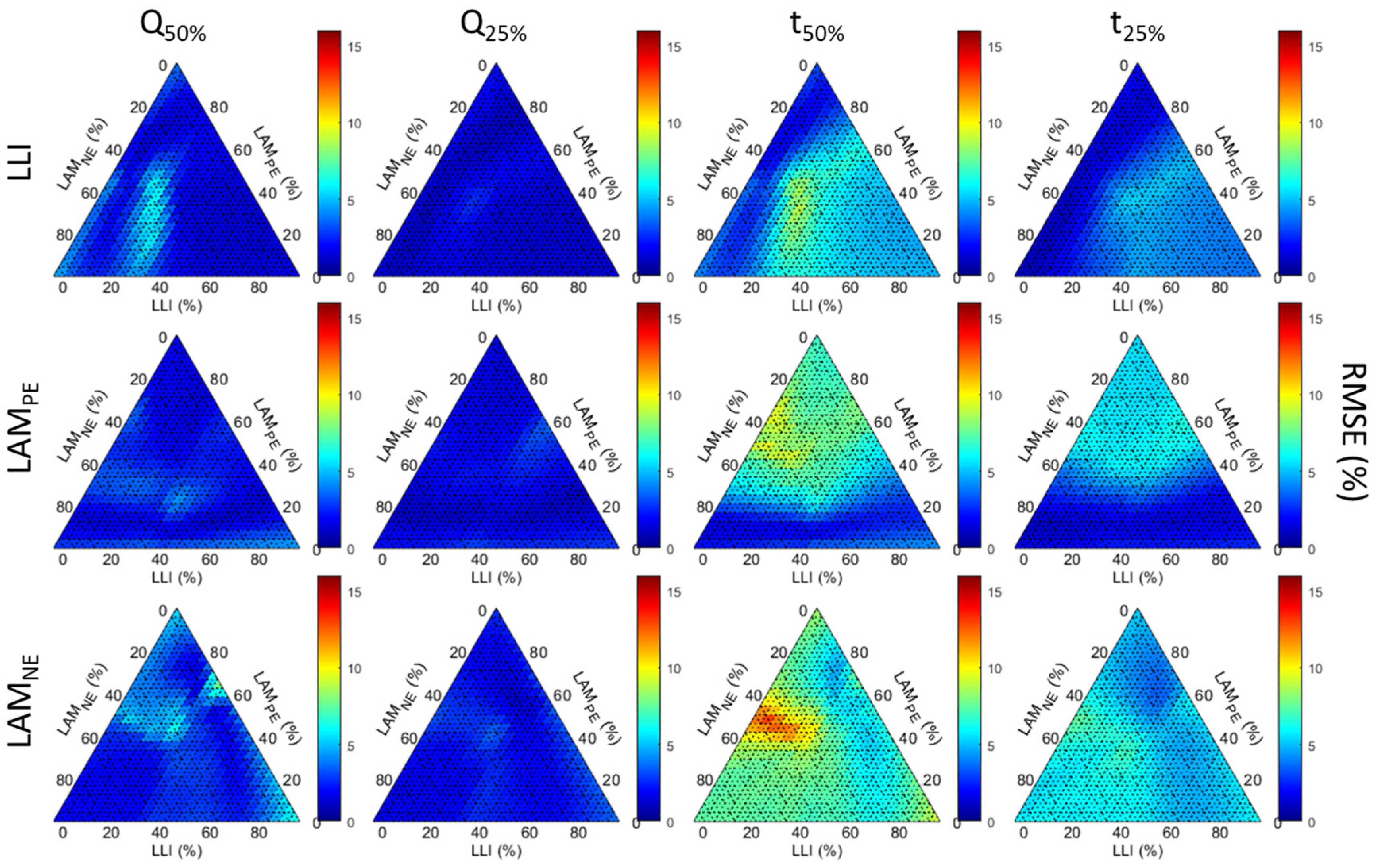
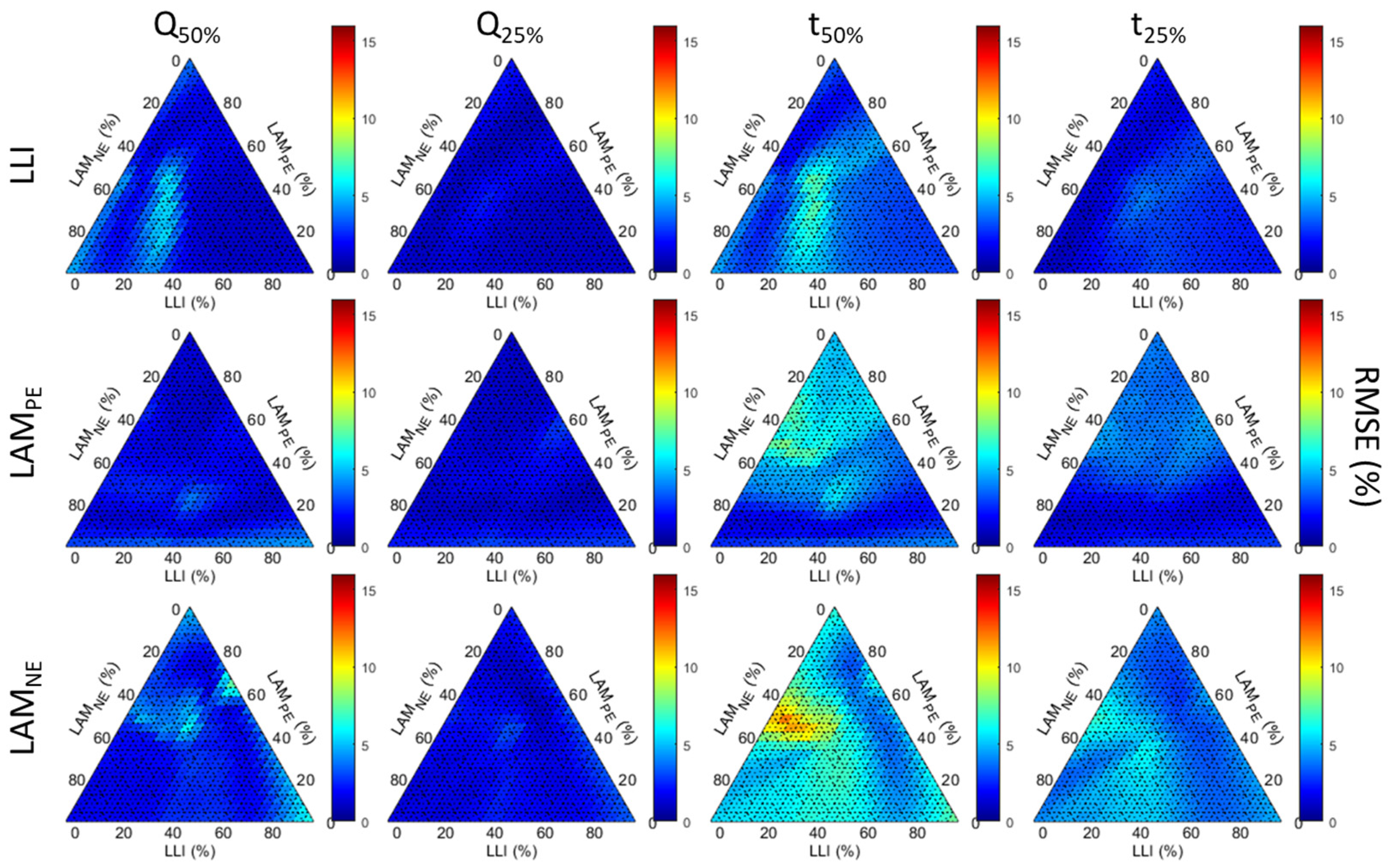
Figure 6 presents the impact of the degradation modes on the diagnosis accuracy for days with 50% or more cs%. The first and third columns summarize every path up to 50% degradation for the Q-based and t-based diagnoses, respectively. The second and fourth columns contain the same data but with up to 25% degradation. The three lines showcase the data for the three degradation modes from top to bottom: LLI, LAMPE, and LAMNE. The same data for other studied case figures (the full dataset, over 70% cs%, |Irr| over 500 W/m2, 600 W/m2, and 650 W/m2) is provided in Figure A1, Figure A2, Figure A3, Figure A4 and Figure A5, respectively. To ease the comparison, every figure uses the same color scheme and scale.
For all case figures except the full dataset, the RMSE of Q-based diagnosis was relatively independent of the degradation composition, as a mainly uniform color is observed throughout the triangles, indicating little impact of the degradation composition on accuracy, especially for the Q-25% diagnosis. For the Q-50% diagnosis, the RMSEs were only slightly higher for LLI estimation when the degradation was dominated by LAMNE (>0.4) with significant LAMPE (up to 0.6) and with between 0.25 and 0.33 of LLI (the white “cloud” on the blue triangle on the top left figure). There was also another small cluster of lower accuracies for LAMNE estimation for degradation, with 0.5 to 0.6 LAMPE and 0.3 to 0.4 LAMNE with little LLI. There was little difference between the four case figures, with only a whiter “cloud” for the less restrictive conditions (50 cs%, |Irr| over 500 W/m2 and 600 W/m2). When the full dataset was considered (Figure A1), there was, however, a clear impact of the degradation composition. For LLI estimation, the “cloud” was still there with the worst accuracy, but RMSEs also increased significantly for all degradations with a fraction of LLI over 0.2. For LAMPE and LAMNE, the best results were obtained for the lower fraction of the respective modes. Looking at the same evolution for the t-based diagnosis, there was more impact from the degradation composition and more difference between the case figures, especially for LAMPE and LAMNE. This time the |Irr| over 500 W/m2 was much closer to the full dataset than the other ones, with RMSEs increasing significantly when the content of the corresponding modes was increasing over 0.2; this was more intense for LAMPE and LAMNE compared to LLI. The |Irr| over 600 W/m2 showcased the same results to a lesser extent, and the clusters identified above for LLI and LAMNE estimation were starting to be visible. These trends continued for the best-case figures, and, except for LLI, the level of path independence reached for Q-based diagnosis cannot be reached for t-based diagnosis.
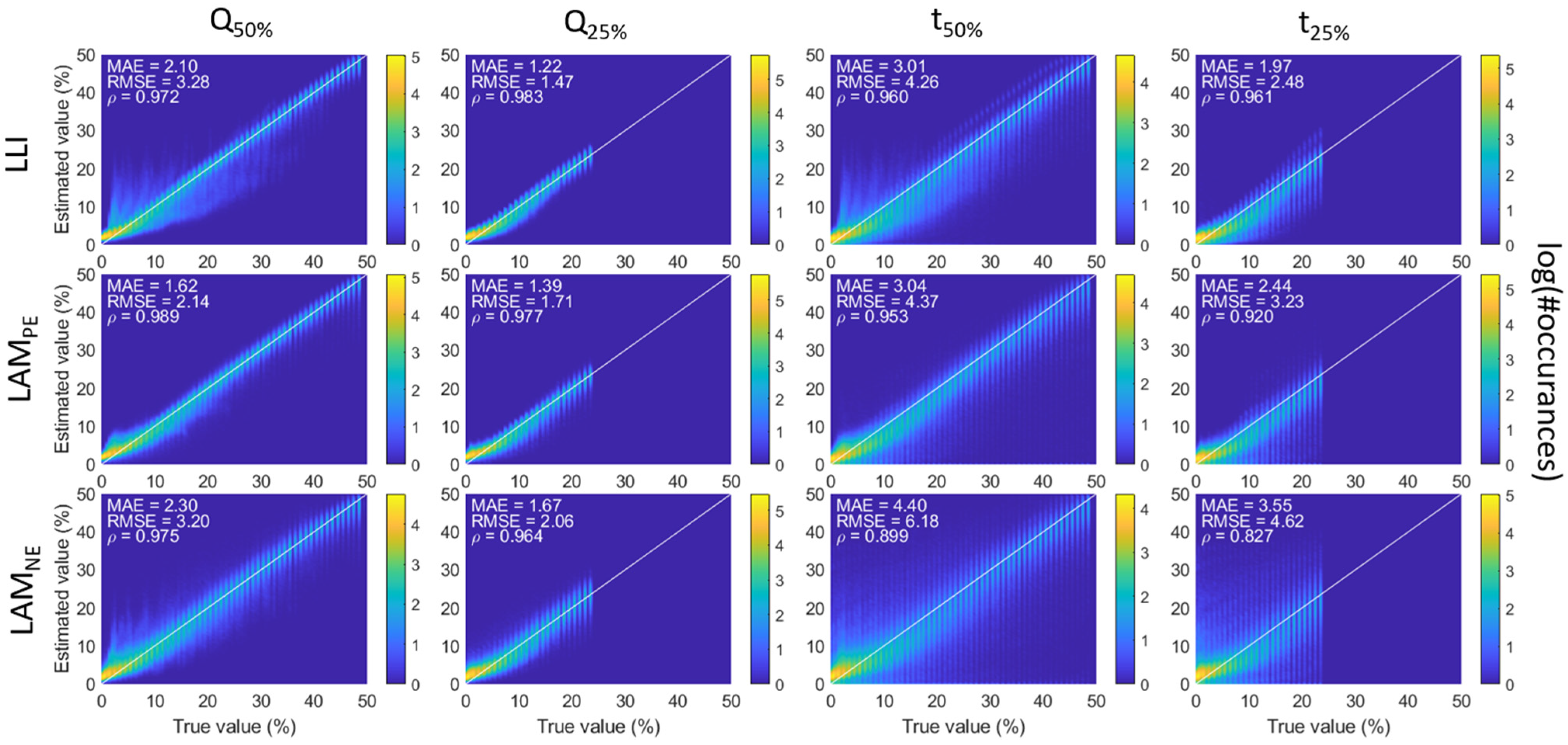
Outside of the full dataset, the analysis of Figure 6 and associated supplementary figures showcased a limited effect of the degradation composition on the Q-based diagnosis and a slight effect on the t-based diagnosis, with the exception of a few clusters. One possibility to explain the clusters is the extent of the degradation, as every point on the triangle corresponds to the average RMSE over up to 25 or 50% degradation, as explained above. It is therefore also important to investigate the evolution of the estimated value as a function of the true value with increasing degradation percentages. Since the results were similar for all case figures except the full dataset, only one condition will be discussed in detail: the one for days over 50% cs% (Figure 7), with the corresponding curves for the full dataset provided in Figure A6. The first noticeable feature to notice is that, similarly to what was reported in [34], there was a haze for low degradation that disappeared, then the maximum degradation was reduced from 50% to 25%. This indicates that the larger errors correspond to degradation paths where one of the modes is low and at least one of the other is high. This corresponds to the position of the “clouds” on Figure 6 (low LLI, high LAMs). This probably explains most of the differences in accuracy between the 50% and 25% degradation datasets since the data for the 25% to 50% degradation range did not showcase any haze and showed a similar distribution around the 1:1 line to the lower ones for the 25% maximum figures. This distribution was much smaller for the Q-based diagnosis compared to the t-based ones, where significant under-estimations occurred (intensity present below the 1:1 line). This impact was much worse on the full data set than on the other ones. Overall, the distribution was also wider for LAMNE estimation than for LAMPE and LLI, but it remained pretty consistent, and there was no sign of clusters of inaccuracies. The clusters observed for specific compositions (Figure 6) are therefore most likely imputable to the algorithm not being able to recognize some degradation compositions.
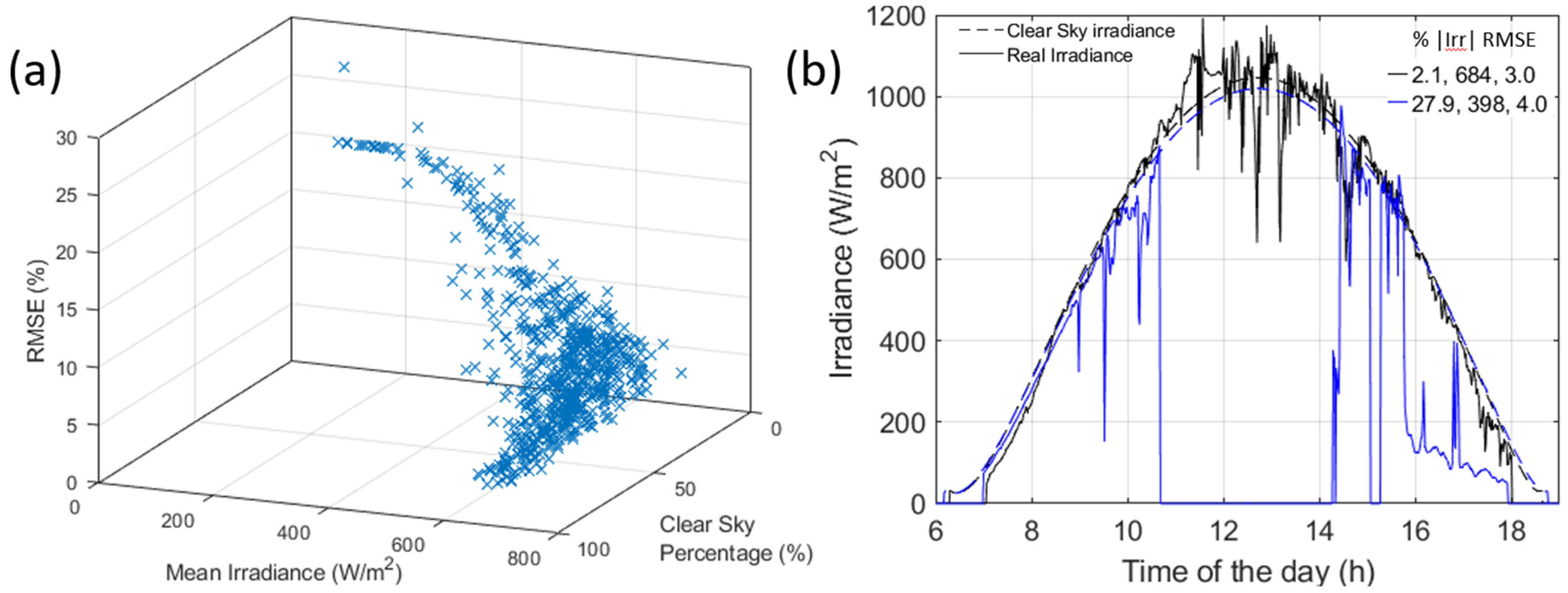
From the results compiled in Table 1 and the impact of the degradation path as well as the extent of the degradation discussed, the different case figures can now be compared in detail to determine what is the best strategy to identify which days should be considered for opportunistic diagnosis. Clearly, the full data set cannot be used, as the overall statistics are not good enough to guarantee an accurate diagnosis. |Irr| over 500 W/m2 (top 75% of the data) and over 600 W/m2 (top 40% of the data) helps improve the statistics to a level where Q-based diagnosis might be an option but not the t-based one. Over 50% cs% (20.5% of the data) and |Irr| over 650 W/m2 (11.5% of the data) present similar results and better diagnosability for t-based data, with a slight advantage for the over 50% cs%. Overall, the best results were obtained for over 70 cs% of the sample, but this only corresponds to 6% of the dataset. Therefore, the best option to detect useful days seems to be the cs%, and the higher it is, the better the accuracy of the diagnosis will be. However, days with high |Irr| could also be used to complement. Looking closer at the over 50% cs% and over 650 W/m2 |Irr| filters, there is only a partial overlap of the days matching the description. Combining both corresponds to 23% of the dataset with RMSEs similar to those of the individual ones. This is because some days with high |Irr| might have low cs% and inversely. For comparison, Figure 8a presents the evolution of the RMSE as a function of both the cs% and the |Irr|. From this figure, it can be seen that the cs% is always low and the RMSE is always high when the |Irr| is below 500 W/m2. For higher |Irr|, every value of cs% seems to be possible. This corresponds to days where the irradiance is close but not matching the modeled one. An example of such a day is presented in Figure 8b, with the black curve. On this day, the cloud coverage prevented the irradiance from being at the clear sky level (cs% = 2%), yet the average irradiance is high (684 W/m2) and the RMSE is low (3% for up to 50% degradation). The cloud cover on this day was likely all very high cirrus clouds, which are more transparent than the typical cumulus and stratocumulus found above Hawaii. This exemplifies that there are some days with high |Irr| but low cs%. Figure 8b also presents another interesting example with the blue curve. This particular day had a low cs% (28%), a low |Irr| (398 W/m2), and yet a low RMSE (4% for up to 50% degradation). Clearly, there was significant cloud coverage mid-day, but this did not prevent diagnosability because only little capacity was exchanged, similar to what was observed in Figure 2. This will, of course, be algorithm, battery size, and chemistry-dependent.
5. Conclusions and Outlook
This work took a deeper dive into the opportunistic PV-connected battery diagnosis technique we recently proposed [34]. By analyzing the statistic obtained from 10,000 degradation paths simulated from 0 to 50% degradation and applied to 720 different days, we were able to confirm that the clear sky percentage is a good metric to detect opportunities but that it could be supplemented by days with high average irradiance. Diagnosis is possible on a capacity basis for days with more than 50% clear sky with limited impact of the degradation composition and extent. For time-based diagnosis, a higher clear-sky percentage is necessary. The limited impact of the composition and extent makes the method particularly attractive for deployment in automated analysis since it will not be sensitive to path dependence and history, which could remove concerns about accuracy under unpredictable conditions. This confirms that the potential benefits of this technique for the community are significant.
Finally, while this analysis provided remarkable new insight into the application of the technique, it also raised a lot of questions that will need to be addressed in future work to move from the academic to the applicable stage. Some obvious ones include the need to consider the impact of imbalance and inhomogeneities in battery packs on the voltage response as well as the impact of the additional usage on cells that will be associated with the eventual usage of the cells while in charge. Before looking into those, it might be interesting to also look into the impact of the PV/battery size ratio, as the results presented here are only valid for the chosen battery chemistry and size relative to the PV. A larger battery will charge slower and might only be partially charged every day, which could limit the information available for the algorithm. A smaller battery will charge faster, which will make diagnosis more complicated because kinetics will play a larger role. While the location will have an impact, we would argue that testing in the tropics is the worst-case scenario with only a reduced season signal relative to locations farther away from the equator where winter days will receive less power, which will result in slower charges and thus easier diagnosis for a similar PV/battery size match. In addition to the rate, the battery size and chemistry will also influence around what time of the day the most prominent voltage features occur, which could affect the diagnosability. A solution could be to create a synthetic benchmark irradiance dataset that covers most possible cloud conditions at different times of the day to test the applicability and limitations of the machine learning algorithm. Speaking of the latter, the current algorithms were developed for constant current applications, and they could be optimized to better address the challenges associated with irradiance data both on capacity and time scales.
Author Contributions
Conceptualization, M.D.; methodology, M.D.; software, M.D., N.C. and D.M.; validation, M.D. and F.Y.; formal analysis, M.D. and F.Y.; investigation, M.D.; resources, M.D.; data curation, M.D.; writing—original draft preparation, M.D.; writing—review and editing, M.D., F.Y., N.C. and D.M.; visualization, M.D.; supervision, M.D.; project administration, M.D.; funding acquisition, M.D. All authors have read and agreed to the published version of the manuscript.
Funding
This work was funded by the Office of Naval Research (ONR) grant number N00014-19-1-2159.
Data Availability Statement
A data sample (18 days) is available here [40,41]. The source code for CNN is available on a public git repository: https://github.com/NahuelCostaCortez/PVDiagnosis, last accessed 26 July 2023.
Acknowledgments
The authors are thankful to ONR for funding the deployment and monitoring of the PV system used in this work with the help of HNEI’s Severine Busquet, Jonathan Kobayashi, and Richard Rocheleau. Finally, the authors would also like to thank Sara Matthews for her insightful comments.
Conflicts of Interest
The authors declare no conflict of interest.
Appendix A
Figure A1.
Diagnosis accuracy for the full dataset as a function of the degradation path for LLI (1st row), LAMPE (2nd row), and LAMNE (3rd row) for Q-based diagnoses to 50% and 25% total degradation (columns 1 and 2) as well as for t-based diagnoses under same conditions (columns 3 and 4).
Figure A1.
Diagnosis accuracy for the full dataset as a function of the degradation path for LLI (1st row), LAMPE (2nd row), and LAMNE (3rd row) for Q-based diagnoses to 50% and 25% total degradation (columns 1 and 2) as well as for t-based diagnoses under same conditions (columns 3 and 4).

Figure A2.
Diagnosis accuracy days with over 70% cs% as a function of the degradation path for LLI (1st row), LAMPE (2nd row), and LAMNE (3rd row) for Q-based diagnoses to 50% and 25% total degradation (columns 1 and 2) as well as for t-based diagnoses under same conditions (columns 3 and 4).
Figure A2.
Diagnosis accuracy days with over 70% cs% as a function of the degradation path for LLI (1st row), LAMPE (2nd row), and LAMNE (3rd row) for Q-based diagnoses to 50% and 25% total degradation (columns 1 and 2) as well as for t-based diagnoses under same conditions (columns 3 and 4).

Figure A3.
Diagnosis accuracy days with over 500 W/m2 average irradiance as a function of the degradation path for LLI (1st row), LAMPE (2nd row), and LAMNE (3rd row) for Q-based diagnoses to 50% and 25% total degradation (columns 1 and 2) as well as for t-based diagnoses under same conditions (columns 3 and 4).

Figure A4.
Diagnosis accuracy days with over 600 W/m2 average irradiance as a function of the degradation path for LLI (1st row), LAMPE (2nd row), and LAMNE (3rd row) for Q-based diagnoses to 50% and 25% total degradation (columns 1 and 2) as well as for t-based diagnoses under same conditions (columns 3 and 4).

Figure A5.
Diagnosis accuracy days with over 650 W/m2 average irradiance as a function of the degradation path for LLI (1st row), LAMPE (2nd row), and LAMNE (3rd row) for Q-based diagnoses to 50% and 25% total degradation (columns 1 and 2) as well as for t-based diagnoses under same conditions (columns 3 and 4).

Figure A6.
Distribution of LLI (1st row), LAMPE (2nd row), and LAMNE (3rd row) estimations vs. true values for the full dataset and Q-based diagnoses to 50% and 25% total degradation (columns 1 and 2) as well as for t-based diagnoses under same conditions (columns 3 and 4).
Figure A6.
Distribution of LLI (1st row), LAMPE (2nd row), and LAMNE (3rd row) estimations vs. true values for the full dataset and Q-based diagnoses to 50% and 25% total degradation (columns 1 and 2) as well as for t-based diagnoses under same conditions (columns 3 and 4).

Appendix B
Battery digital twin model parameters:
- -
- PE: NMC111, NE: graphite
- -
- Rate independent: Loading ratio: 1.2, Offset: 4, Resistance adjustment: −0.1,
- -
- Rate dependent:
- o
- Rate degradation factor for the PE: 0.064.rate−0.836,
- o
- Rate degradation factor for the NE: 0.443.rate−0.217,
- o
- Rate degradation factor correction for the PE: 3.916.rate−0.306.
References
- Wood Mackenzie/SEIA. US Solar Market Insight; Wood Mackenzie/SEIA: Edinburgh, UK, 2021. [Google Scholar]
- EIA. Battery Storage in the United States: An Update on Market Trends; EIA: Washington, DC, USA, 2021. [Google Scholar]
- Che, Y.; Hu, X.; Lin, X.; Guo, J.; Teodorescu, R. Health prognostics for lithium-ion batteries: Mechanisms, methods, and prospects. Energy Environ. Sci. 2023, 16, 338–371. [Google Scholar] [CrossRef]
- Vasta, E.; Scimone, T.; Nobile, G.; Eberhardt, O.; Dugo, D.; De Benedetti, M.M.; Lanuzza, L.; Scarcella, G.; Patanè, L.; Arena, P.; et al. Models for Battery Health Assessment: A Comparative Evaluation. Energies 2023, 16, 632. [Google Scholar] [CrossRef]
- Barrett, D.H.; Haruna, A. Artificial intelligence and machine learning for targeted energy storage solutions. Curr. Opin. Electrochem. 2020, 21, 160–166. [Google Scholar] [CrossRef]
- Cui, Z.; Wang, L.; Li, Q.; Wang, K. A comprehensive review on the state of charge estimation for lithium-ion battery based on neural network. Int. J. Energ. Res. 2021, 46, 5423–5440. [Google Scholar] [CrossRef]
- Sharma, P.; Bora, B.J. A Review of Modern Machine Learning Techniques in the Prediction of Remaining Useful Life of Lithium-Ion Batteries. Batteries 2022, 9, 13. [Google Scholar] [CrossRef]
- Rauf, H.; Khalid, M.; Arshad, N. Machine learning in state of health and remaining useful life estimation: Theoretical and technological development in battery degradation modelling. Renew. Sustain. Energy Rev. 2022, 156, 11190. [Google Scholar] [CrossRef]
- Na, H.S.; Numan-Al-Mobin, A.M. Machine learning approaches to estimate the health state of next-generation energy storage. In Green Sustainable Process for Chemical and Environmental Engineering and Science; Elsevier: Amsterdam, The Netherlands, 2023; pp. 343–363. [Google Scholar]
- Severson, K.A.; Attia, P.M.; Jin, N.; Perkins, N.; Jiang, B.; Yang, Z.; Chen, M.H.; Aykol, M.; Herring, P.K.; Fraggedakis, D.; et al. Data-driven prediction of battery cycle life before capacity degradation. Nat. Energy 2019, 4, 383–391. [Google Scholar] [CrossRef] [Green Version]
- dos Reis, G.; Strange, C.; Yadav, M.; Li, S. Lithium-ion battery data and where to find it. Energy AI 2021, 5, 100081. [Google Scholar] [CrossRef]
- Ward, L.; Babinec, S.; Dufek, E.J.; Howey, D.A.; Viswanathan, V.; Aykol, M.; Beck, D.A.C.; Blaiszik, B.; Chen, B.-R.; Crabtree, G.; et al. Principles of the Battery Data Genome. Joule 2022, 6, 2253–2271. [Google Scholar] [CrossRef]
- Preger, Y.; Barkholtz, H.M.; Fresquez, A.; Campbell, D.L.; Juba, B.W.; Romàn-Kustas, J.; Ferreira, S.R.; Chalamala, B.R. Degradation of Commercial Lithium-ion Cells as a Function of Chemistry and Cycling Conditions. J. Electrochem. Soc. 2020, 167, 120532. [Google Scholar] [CrossRef]
- Dubarry, M.; Beck, D. Big data training data for artificial intelligence-based Li-ion diagnosis and prognosis. J. Power Sources 2020, 479, 228806. [Google Scholar] [CrossRef]
- Aykol, M.; Gopal, C.B.; Anapolsky, A.; Herring, P.K.; van Vlijmen, B.; Berliner, M.D.; Bazant, M.Z.; Braatz, R.D.; Chueh, W.C.; Storey, B.D. Perspective—Combining Physics and Machine Learning to Predict Battery Lifetime. J. Electrochem. Soc. 2021, 168, 030525. [Google Scholar] [CrossRef]
- Doyle, M.; Newman, J.; Gozdz, A.S.; Schmutz, C.N.; Tarascon, J.M. Comparison of Modeling Predictions with Experimental Data from Plastic Lithium Ion Cells. J. Electrochem. Soc. 1996, 143, 1890–1903. [Google Scholar] [CrossRef]
- Wang, A.; O’Kane, S.; Brosa Planella, F.; Le Houx, J.; O’Regan, K.; Zyskin, M.; Edge, J.S.; Monroe, C.; Cooper, S.; Howey, D.A.; et al. Review of parameterisation and a novel database (LiionDB) for continuum Li-ion battery models. Progress Energy 2022, 4, 032004. [Google Scholar] [CrossRef]
- Sarkar, S.; Zohra Halim, S.; El-Halwagi, M.M.; Khan, F.I. Electrochemical models: Methods and applications for safer lithium-ion battery operation. J. Electrochem. Soc. 2022, 169, 100501. [Google Scholar] [CrossRef]
- Tu, H.; Moura, S.; Wang, Y.; Fang, H. Integrating physics-based modeling with machine learning for lithium-ion batteries. Appl. Energy 2023, 329, 120289. [Google Scholar] [CrossRef]
- Hofmann, T.; Hamar, J.; Rogge, M.; Zoerr, C.; Erhard, S.; Schmidt, J.P. Physics-Informed Neural Networks for State of Health Estimation in Lithium-Ion Batteries. J. Power Sources 2023, preprint. [Google Scholar]
- Zhang, Y.; Feng, X.; Zhao, M.; Xiong, R. In-situ battery life prognostics amid mixed operation conditions using physics-driven machine learning. J. Power Sources 2023, 577, 233246. [Google Scholar] [CrossRef]
- Honkura, K.; Takahashi, K.; Horiba, T. Capacity-fading prediction of lithium-ion batteries based on discharge curves analysis. J. Power Sources 2011, 196, 10141–10147. [Google Scholar] [CrossRef]
- Bloom, I.; Jansen, A.N.; Abraham, D.P.; Knuth, J.; Jones, S.A.; Battaglia, V.S.; Henriksen, G.L. Differential voltage analyses of high-power, lithium-ion cells. 1. Technique and Applications. J. Power Sources 2005, 139, 295–303. [Google Scholar] [CrossRef]
- Dubarry, M.; Truchot, C.; Liaw, B.Y. Synthesize battery degradation modes via a diagnostic and prognostic model. J. Power Sources 2012, 219, 204–216. [Google Scholar] [CrossRef]
- Birkl, C.R.; Roberts, M.R.; McTurk, E.; Bruce, P.G.; Howey, D.A. Degradation diagnostics for lithium ion cells. J. Power Sources 2017, 341, 373–386. [Google Scholar] [CrossRef]
- Dubarry, M.; Berecibar, M.; Devie, A.; Anseán, D.; Omar, N.; Villarreal, I. State of health battery estimator enabling degradation diagnosis: Model and algorithm description. J. Power Sources 2017, 360, 59–69. [Google Scholar] [CrossRef]
- Dubarry, M.; Beck, D. Analysis of Synthetic Voltage vs. Capacity Datasets for Big Data Li-ion Diagnosis and Prognosis. Energies 2021, 14, 2371. [Google Scholar] [CrossRef]
- Kim, S.; Yi, Z.; Chen, B.-R.; Tanim, T.R.; Dufek, E.J. Rapid failure mode classification and quantification in batteries: A deep learning modeling framework. Energy Storage Mater. 2022, 45, 1002–1011. [Google Scholar] [CrossRef]
- Mayilvahanan, K.S.; Takeuchi, K.J.; Takeuchi, E.S.; Marschilok, A.C.; West, A.C. Supervised Learning of Synthetic Big Data for Li-Ion Battery Degradation Diagnosis. Batter. Supercaps 2021, 5, e202100166. [Google Scholar] [CrossRef]
- Costa, N.; Sanchez, L.; Ansean, D.; Dubarry, M. Li-ion battery degradation modes diagnosis via Convolutional Neural Networks. J. Energy Storage 2022, accepted. [Google Scholar] [CrossRef]
- Kim, S.; Jung, H.; Lee, M.; Choi, Y.Y.; Choi, J.-I. Model-free reconstruction of capacity degradation trajectory of lithium-ion batteries using early cycle data. eTransportation 2023, 17, 100243. [Google Scholar] [CrossRef]
- Ruan, H.; Chen, J.; Ai, W.; Wu, B. Generalised diagnostic framework for rapid battery degradation quantification with deep learning. Energy AI 2022, 9, 100158. [Google Scholar] [CrossRef]
- Dubarry, M.; Beck, D. Perspective on Mechanistic Modeling of Li-Ion Batteries. Acc. Mater. Res. 2022, 3, 843–853. [Google Scholar] [CrossRef]
- Dubarry, M.; Costa, N.; Matthews, D. Data-driven direct diagnosis of Li-ion batteries connected to photovoltaics. Nat. Commun. 2023, 14, 3138. [Google Scholar] [CrossRef] [PubMed]
- Ineichen, P.; Perez, R. A new airmass independent formulation for the Linke turbidity coefficient. Sol. Energy 2002, 73, 151–157. [Google Scholar] [CrossRef] [Green Version]
- Liu, B.Y.H.; Jordan, R.C. The interrelationship and characteristic distribution of direct, diffuse and total solar radiation. Sol. Energy 1960, 4, 1–19. [Google Scholar] [CrossRef]
- Loutzenhiser, P.G.; Manz, H.; Felsmann, C.; Strachan, P.A.; Frank, T.; Maxwell, G.M. Empirical validation of models to compute solar irradiance on inclined surfaces for building energy simulation. Sol. Energy 2007, 81, 254–267. [Google Scholar] [CrossRef] [Green Version]
- Devie, A.; Dubarry, M. Durability and Reliability of Electric Vehicle Batteries under Electric Utility Grid Operations. Part 1: Cell-to-Cell Variations and Preliminary Testing. Batteries 2016, 2, 28. [Google Scholar] [CrossRef] [Green Version]
- Abadi, M.; Barham, P.; Chen, J.; Chen, Z.; Davis, A.; Dean, J.; Devin, M.; Ghemawat, S.; Irving, G.; Isard, M.; et al. TensorFlow: A system for large-scale machine learning. In Proceedings of the 12th USENIX Symposium on Operating Systems Design and Implementation (OSDI ‘16), Savannah, GA, USA, 2–4 November 2016. [Google Scholar]
- Dubarry, M.; Costa, N.; Matthews, D. GIC//NMC Solar Battery Synthetic Data 1—700,000 degradation for 03/21 clear-sky irradiance. Mendeley Data 2022, 1. [Google Scholar] [CrossRef]
- Dubarry, M.; Costa, N.; Matthews, D. GIC//NMC Solar Battery Synthetic Data 2—45,000 × 18 degradation for clear-sky irradiance and cloudy days. Mendeley Data 2022, 1. [Google Scholar] [CrossRef]
Figure 1.
Schematic summary of the approach.

Figure 2.
Example of the data used in this work for the observed and clear sky irradiance with (a) the observed irradiance for a randomly selected day from the dataset (22 May 2017), (b) voltage/rate calculations to match the requested power, (c) the resulting voltage response for the cells as a function of capacity with the associated incremental capacity curve as an inset, and (d) the voltage response as a function of time with the associated dt/dV vs. V curve as an inset.

Figure 3.
Distribution of (a,b) the clear sky percentage and (c,d) the average irradiance for the entire 2-year dataset and per season, respectively.
Figure 3.
Distribution of (a,b) the clear sky percentage and (c,d) the average irradiance for the entire 2-year dataset and per season, respectively.

Figure 4.
Detailed RMSE evolution as a function of the percentage of clear sky for capacity-based diagnosis up to (a) 50% and (c) 25% degradation and time-based diagnosis up to (b) 50% and (d) 25% degradation. Some outliers were present above the 35% cutoff.
Figure 4.
Detailed RMSE evolution as a function of the percentage of clear sky for capacity-based diagnosis up to (a) 50% and (c) 25% degradation and time-based diagnosis up to (b) 50% and (d) 25% degradation. Some outliers were present above the 35% cutoff.

Figure 5.
Detailed RMSE evolution as a function of the average irradiance for capacity-based diagnosis up to (a) 50% and (c) 25% degradation and time-based diagnosis up to (b) 50% and (d) 25% degradation. Some outliers were present above the 35% cutoff.
Figure 5.
Detailed RMSE evolution as a function of the average irradiance for capacity-based diagnosis up to (a) 50% and (c) 25% degradation and time-based diagnosis up to (b) 50% and (d) 25% degradation. Some outliers were present above the 35% cutoff.

Figure 6.
Diagnosis accuracy for days with >50% cs% as a function of the degradation path for LLI (1st row), LAMPE (2nd row), and LAMNE (3rd row) for Q-based diagnoses to 50% and 25% total degradation (columns 1 and 2) as well as for t-based diagnoses to 50% and 25% total degradation (columns 3 and 4).

Figure 7.
Distribution of LLI (1st row), LAMPE (2nd row), and LAMNE (3rd row) estimations vs. true values for the days with over 50% cs% and Q-based diagnoses to 50% and 25% total degradation (columns 1 and 2) as well as for t-based diagnoses under same conditions (columns 3 and 4).
Figure 7.
Distribution of LLI (1st row), LAMPE (2nd row), and LAMNE (3rd row) estimations vs. true values for the days with over 50% cs% and Q-based diagnoses to 50% and 25% total degradation (columns 1 and 2) as well as for t-based diagnoses under same conditions (columns 3 and 4).

Figure 8.
(a) average RMSE vs. cs% vs. average irradiance; and (b) examples of days with low RMSE while having low cs% or low average irradiance.
Figure 8.
(a) average RMSE vs. cs% vs. average irradiance; and (b) examples of days with low RMSE while having low cs% or low average irradiance.


Table 1.
Statistics Metrics Summary.
| Q50 | Q25 | t50 | t25 | ||||||||||
|---|---|---|---|---|---|---|---|---|---|---|---|---|---|
| RMSE (%) | MAE (%) | Ρ | RMSE (%) | MAE (%) | ρ | RMSE (%) | MAE (%) | ρ | RMSE (%) | MAE (%) | ρ | ||
| LLI | Full | 4.90 | 3.43 | 0.93 | 2.96 | 2.27 | 0.88 | 9.40 | 7.00 | 0.80 | 6.42 | 4.74 | 0.74 |
| >50% cs | 3.28 | 2.10 | 0.97 | 1.47 | 1.22 | 0.98 | 4.26 | 3.01 | 0.96 | 2.48 | 1.97 | 0.96 | |
| >70% cs | 3.24 | 2.06 | 0.97 | 1.45 | 1.21 | 0.98 | 3.84 | 2.66 | 0.96 | 2.12 | 1.70 | 0.97 | |
| >600 W/m2 | 3.42 | 2.23 | 0.97 | 1.58 | 1.29 | 0.98 | 5.12 | 3.74 | 0.95 | 3.25 | 2.52 | 0.95 | |
| >650 W/m2 | 3.34 | 2.15 | 0.97 | 1.48 | 1.23 | 0.98 | 4.33 | 3.07 | 0.96 | 2.42 | 1.93 | 0.96 | |
| LAMPE | Full | 5.34 | 3.93 | 0.89 | 4.19 | 3.17 | 0.80 | 10.70 | 7.85 | 0.74 | 7.47 | 5.50 | 0.64 |
| >50% cs | 2.14 | 1.62 | 0.99 | 1.71 | 1.39 | 0.98 | 4.37 | 3.04 | 0.95 | 3.23 | 2.44 | 0.92 | |
| >70% cs | 1.97 | 1.50 | 0.99 | 1.61 | 1.31 | 0.98 | 3.75 | 2.55 | 0.96 | 2.81 | 2.08 | 0.93 | |
| >600 W/m2 | 2.54 | 1.90 | 0.99 | 1.92 | 1.54 | 0.97 | 5.64 | 4.03 | 0.93 | 4.07 | 3.05 | 0.89 | |
| >650 W/m2 | 2.22 | 1.67 | 0.99 | 1.70 | 1.39 | 0.98 | 4.45 | 3.06 | 0.95 | 3.07 | 2.30 | 0.93 | |
| LAMNE | Full | 5.97 | 4.30 | 0.87 | 4.07 | 3.08 | 0.78 | 11.85 | 8.49 | 0.64 | 8.34 | 5.94 | 0.50 |
| >50% cs | 3.20 | 2.30 | 0.98 | 2.06 | 1.67 | 0.96 | 6.18 | 4.40 | 0.90 | 4.62 | 3.55 | 0.83 | |
| >70% cs | 2.98 | 2.14 | 0.98 | 1.88 | 1.54 | 0.97 | 4.97 | 3.42 | 0.94 | 3.38 | 2.56 | 0.90 | |
| >600 W/m2 | 3.56 | 2.55 | 0.97 | 2.30 | 1.84 | 0.95 | 7.43 | 5.37 | 0.86 | 5.21 | 3.96 | 0.76 | |
| >650 W/m2 | 3.27 | 2.34 | 0.97 | 2.05 | 1.66 | 0.96 | 6.17 | 4.43 | 0.91 | 4.26 | 3.26 | 0.85 | |
| Mean | Full | 5.40 | 3.89 | 0.90 | 3.74 | 2.84 | 0.82 | 10.65 | 7.78 | 0.73 | 7.41 | 5.39 | 0.63 |
| >50% cs | 2.87 | 2.00 | 0.98 | 1.75 | 1.43 | 0.97 | 4.94 | 3.48 | 0.94 | 3.44 | 2.65 | 0.90 | |
| >70% cs | 2.73 | 1.90 | 0.98 | 1.65 | 1.35 | 0.98 | 4.19 | 2.88 | 0.96 | 2.77 | 2.12 | 0.93 | |
| >600 W/m2 | 3.17 | 2.22 | 0.97 | 1.93 | 1.56 | 0.97 | 6.06 | 4.38 | 0.91 | 4.18 | 3.18 | 0.86 | |
| >650 W/m2 | 2.95 | 2.05 | 0.98 | 1.74 | 1.43 | 0.97 | 4.98 | 3.52 | 0.94 | 3.25 | 2.50 | 0.91 | |
Disclaimer/Publisher’s Note: The statements, opinions and data contained in all publications are solely those of the individual author(s) and contributor(s) and not of MDPI and/or the editor(s). MDPI and/or the editor(s) disclaim responsibility for any injury to people or property resulting from any ideas, methods, instructions or products referred to in the content. |
© 2023 by the authors. Licensee MDPI, Basel, Switzerland. This article is an open access article distributed under the terms and conditions of the Creative Commons Attribution (CC BY) license (https://creativecommons.org/licenses/by/4.0/).
Share and Cite
MDPI and ACS Style
Dubarry, M.; Yasir, F.; Costa, N.; Matthews, D. Data-Driven Diagnosis of PV-Connected Batteries: Analysis of Two Years of Observed Irradiance. Batteries 2023, 9, 395. https://doi.org/10.3390/batteries9080395
AMA Style
Dubarry M, Yasir F, Costa N, Matthews D. Data-Driven Diagnosis of PV-Connected Batteries: Analysis of Two Years of Observed Irradiance. Batteries. 2023; 9(8):395. https://doi.org/10.3390/batteries9080395
Chicago/Turabian StyleDubarry, Matthieu, Fahim Yasir, Nahuel Costa, and Dax Matthews. 2023. "Data-Driven Diagnosis of PV-Connected Batteries: Analysis of Two Years of Observed Irradiance" Batteries 9, no. 8: 395. https://doi.org/10.3390/batteries9080395
Note that from the first issue of 2016, this journal uses article numbers instead of page numbers. See further details here.