Limit Cycles of Polynomially Integrable Piecewise Differential Systems

Abstract

In this paper, we study how many algebraic limit cycles have the discontinuous piecewise linear differential systems separated by a straight line, with polynomial first integrals on both sides. We assume that at least one of the systems is Hamiltonian. Under this assumption, piecewise differential systems have no more than one limit cycle. This study characterizes linear differential systems with polynomial first integrals.

1. Introduction

We will consider discontinuous piecewise linear differential systems (DPwLS) on the plane ${\mathbb{R}}^2$. On the half plane where x is negative they are expressed as:

$$\left(\begin{array}{c}\dot{x}\\ \dot{y}\end{array}\right)=A^{-}\left(\begin{array}{c}x\\ y\end{array}\right)+b^{-},$$

(1)

and where x is positive as:

$$\left(\begin{array}{c}\dot{x}\\ \dot{y}\end{array}\right)=A^{+}\left(\begin{array}{c}x\\ y\end{array}\right)+b^{+},$$

(2)

where $A^{\pm }$ are real $2\times 2$ matrices and $b^{\pm }\in {\mathbb{R}}^2$. For the definition of a DPwLS on $x=0$, we follow Filippov’s solution [1].

DPwLSs have been studied in depth [2]. An introduction to and a comprehensive list of references can be found in the books [3,4], and the survey [5].

Since planar linear differential systems have no limit cycles (isolated periodic orbits), the limit cycles of DPwLSs separated by a straight line must cross the straight line at two points. In this paper, we do not consider the possible limit cycles which have a segment on the discontinuous straight line, called sliding limit cycles.

The limit cycles of planar differential systems play a main role in understanding the dynamics of such systems, as well as for planar DPwLSs. Thus, the limit cycles of DPwLSs (1) and (2) have been studied intensively in the last twenty years. The current situation of proven bounds is summarized in [6].

One problem still to be solved is: “Is three the maximum number of limit cycles that a discontinuous piecewise linear differential system with a straight line of separation can have?”

Recently, Buzzi, Gasull and Torregrosa analyzed the particular class of algebraic limit cycles in the DPwLS (1) and (2) [7]. They establish that a limit cycle is algebraic if “all its points, except the ones on the sliding set, are contained in the level sets of one or two polynomials”. One of the main results of [7] is to show the existence of DPwLSs (1) and (2) with two algebraic limit cycles.

In order to deal with algebraic limit cycles for DPwLSs, we must work with linear differential systems with polynomial first integrals (PFI) on both sides of $x=0$. Therefore, we need to identify and classify the planar linear differential systems with a PFI. To the best of the authors’ knowledge, such a classification has not been done. In [8], the authors provide a characterization of all quadratic differential systems with a PFI. However, this is not applicable to our area of interest because they do not consider the cases where all the coefficients of the quadratic terms vanish at the same time. Below, we classify all the linear differential systems with PFIs.

Theorem 1.

Let us consider system

$$\begin{array}{c}\dot{x}=a+bx+cy,\hfill \\ \dot{y}=d+ex+fy,\hfill \end{array}$$

(3)

with at most one equilibrium point (the associated vector field has no common factors) and where $b^2+c^2+e^2+f^2\ne 0$. This system has a PFI $H(x,y)$ if and only if one of the following conditions hold.

(i) 

If $f=-b$, then $H_1(x,y)=e{x}^2-c{y}^2-2bxy+2dx-2ay$.

(ii) 

If $f\ne -b$, $c\ne 0$, $ec\ne fb$ and there are two positive integers, p and q, such that $p\ne q$ and $ce=(pb+qf)(pf+qb)/{(q-p)}^2$, then

$$\begin{array}{cc}\hfill H_2(x,y)=& {\left(cy+{\displaystyle \frac{pf+qb}{q-p}}x+{\displaystyle \frac{a(pf+qb)+dc(q-p)}{q(f+b)}}\right)}^p\hfill \\ & {\left(cy-{\displaystyle \frac{pb+qf}{q-p}}x+{\displaystyle \frac{a(pb+qf)-dc(q-p)}{p(f+b)}}\right)}^q.\hfill \end{array}$$

(iii) 

If $fb\ne 0$, $f^2\ne b^2$ and $c=0$ and there are two positive integers p and q such that $p\ne q$ and $pb+qf=0$, then

$$H_3(x,y)={(a+bx)}^p{\left(efx+f(f-b)y+d(f-b)+ae\right)}^q.$$

The main goal of this paper is to characterize the maximum number of limit cycles of DPwLSs such as (1) and (2) formed by two linear differential systems with PFI when at least one of these differential systems is a Hamiltonian system. Our main result is the following.

Theorem 2.

When both linear differential systems, (1) and (2), have a PFI, they have at most one limit cycle if only one of the two systems is Hamiltonian. If both systems are Hamiltonian, then the DPwLS has no limit cycles.

The rest of this paper is organized as follows. Section 2 shows a proof of Theorem 1 following arguments related with factorization and divisibility of polynomials. Section 3 gives the proof of Theorem 2, applying the first integrals of Theorem 1. Finally, in Section 4, we present a DPwLS such as (1) and (2) when both differential systems have a PFI and exactly one limit cycle.

In [9], they study the limit cycles of the discontinuous piecewise differential systems separated by one straight line and formed by two polynomial Hamiltonian systems, and consequently, such limit cycles are algebraic. While in this paper, only one of the systems is Hamiltonian, otherwise the piecewise differential system cannot have limit cycles.

Some authors are interested in knowing if the limit cycles of a discontinuous piecewise differential system persist when the piecewise differential is regularized (see [10]), or how many limit cycles can have such regularized piecewise differential systems (see [11]). For the discontinuous piecewise differential systems studied here, having one algebraic limit cycle, if they are regularized using the regularization of Sotomayor and Teixeira [12], the limit cycle persists but it is no longer algebraic.

2. Proof of Theorem 1

In order to prove Theorem 1, we must introduce a previous result: the polynomial resolution of polynomial differential equations of the form $NH+U{H}_y=0$, where N and U are polynomial and H is a polynomial solution of degree n.

Proposition 1.

We consider the differential equation

$$NH+U{H}_y=0,$$

(4)

where N and U are polynomials, non identically zero and coprime. If $U={\displaystyle \prod _{i=1}^r}{P}_i^{r_i}$ where $P_i$ are the irreducible real factors of U, then (4) has a polynomial solution H of degree n, different from the trivial $H=0$, if and only if there exists $n_1,n_2,\dots ,n_r\in \mathbb{N}$ such that ${\displaystyle \sum _{i=1}^r}{n}_{i}deg{P}_i\le n$ and

$$N+\sum _{j=1}^r{n}_j{P}_{j,y}\frac{U}{P_j}=0.$$

Moreover, when the polynomial H exists, then $H=W{\prod }_{i=1}^r{P}_i^{n_i}$, where W is a polynomial of degree $k=n-{\displaystyle \sum _{i=1}^r}{n}_{i}deg{P}_i$, which does not depend on the variable y. If H is homogeneous, then U and W are homogeneous and $W=\gamma x^k$ with $\gamma \in \mathbb{R}$.

Proof. 

Since N and U are coprime polynomials and H must also be polynomial, it follows that U divides H. So, $n_1,n_2,\dots ,n_r\in \mathbb{N}$ such that $H=RW$ and $R={\displaystyle \prod _{i=1}^r}{P}_i^{n_i}$ with $n_i\ge r_i$. Furthermore, we can assume that R and W are coprime. Taking into account these considerations in (4):

$$\begin{array}{cc}\hfill NH+U{H}_y=& NRW+U\left(\left({\displaystyle \sum _{j=1}^r}{n}_j{P}_j^{n_j-1}{P}_{j,y}{\displaystyle \prod _{i=1,i\ne j}^r}{P}_i^{n_i}\right)W+R{W}_y\right)\hfill \\ \hfill =& NRW+U\left(\left({\displaystyle \sum _{j=1}^r}{n}_j{P}_{j,y}{\displaystyle \frac{R}{P_j}}\right)W+R{W}_y\right)\hfill \\ \hfill =& NRW+R\left(\left({\displaystyle \sum _{j=1}^r}{n}_j{P}_{j,y}{\displaystyle \frac{U}{P_j}}\right)W+U{W}_y\right)=0.\hfill \end{array}$$

Now dividing this equation by R

$$\left(N+\sum _{j=1}^r{n}_j{P}_{j,y}\frac{U}{P_j}\right)W+U{W}_y=0.$$

Since U and W are coprime and $degU>deg\left(N+{\displaystyle \sum _{j=1}^r}{n}_j{P}_{j,y}{\displaystyle \frac{U}{P_j}}\right)$, $N+{\displaystyle \sum _{j=1}^r}{n}_j{P}_{j,y}{\displaystyle \frac{U}{P_j}}=0$ and $W_y=0$. Thus, $W=W\left(x\right)$. Finally, if H is homogeneous then $P_j$ for all $j=1,\dots r$ and W are also homogeneous because all of them are factors of H. Thus, U is homogeneous and $W=\gamma x^k$ where $k=n-{\displaystyle \sum _{i=1}^r}{n}_{i}deg{P}_i$. □

To compute a PFI H of degree n of system (3), we use the decomposition in homogeneous parts of such a PFI.

Proposition 2.

We consider $P(x,y)=\tilde{a}+\tilde{b}x+\tilde{c}y$ and $Q(x,y)=\tilde{d}+\tilde{e}x+\tilde{f}y$ with $P·Q\ne 0$. We suppose that the polynomial differential system

$$\dot{x}=P(x,y),\dot{y}=Q(x,y),$$

(5)

has a PFI H of degree n. This can be expressed as $xQ-yP={\displaystyle \sum _{i=1}^2}{T}_i$, where $T_i$ is the homogeneous part of degree i of the polynomial $xQ-yP$.

If $H={\displaystyle \sum _{i=0}^n}{H}_i$ where $H_i$ is the homogeneous part of degree i of H, then the $H_i$s verify the following system of equations

$$\begin{array}{ccc}\hfill n{P}_1{H}_n+T_2{H}_{n,y}& =& 0,\hfill \\ \hfill (n-1)P_1{H}_{n-1}+T_2{H}_{n-1,y}& =& -(n{P}_0{H}_n+T_1{H}_{n,y}),\hfill \\ \hfill \dots & & \\ \hfill (n-j)P_1{H}_{n-j}+T_2{H}_{n-j,y}& =& -((n-j+1)P_0{H}_{n-j+1}+T_1{H}_{n-j+1,y}),\hfill \\ \hfill \dots & & \\ \hfill P_1{H}_1+T_2{H}_{1,y}& =& -(2P_0{H}_2+T_1{H}_{2,y}),\hfill \\ \hfill 0& =& -(P_0{H}_1+T_1{H}_{1,y}),\hfill \end{array}$$

(6)

where $H_{j,y}$ is the partial derivative of $H_j$ with respect to the variable y and $P_i$ is the homogeneous part of the polynomial P of degree i.

Proof. 

We consider the partial derivatives of H, i.e., $H_x$ and $H_y$. Thus:

$$P{H}_x+Q{H}_y=0.$$

(7)

The Euler Theorem for homogeneous functions gives that

$$x{H}_x+y{H}_y=\sum _{j=1}^n(x{H}_{j,x}+y{H}_{j,y})=\sum _{j=1}^{n}j{H}_j.$$

(8)

Therefore,

$$x{H}_x=\sum _{j=1}^{n}j{H}_j-y{H}_y.$$

(9)

Multiplying Equation (7) by x and substituting $x{H}_x$ with the value given in (9):

$$P\sum _{j=1}^{n}j{H}_j+(xQ-yP)H_y=0.$$

(10)

Finally, taking into account that $P=P_0+P_1$ and $xQ-yP=T_1+T_2$, the homogeneous parts of (10), arranged from the greatest to the lowest degree provide system (6). □

Remark 1.

If system (5) is homogeneous, $\tilde{a}=\tilde{d}=0$, any PFI H verifies that each homogeneous part of H also is a PFI of (5). Therefore, in homogeneous differential systems, it is logical to consider only homogeneous PFI.

Corollary 1.

If system (5) is homogeneous, then any homogeneous PFI H of degree n satisfies $nPH+(xQ-yP)H_y=0$, where $xQ-yP=-\tilde{c}{y}^2+(\tilde{f}-\tilde{b})xy+\tilde{e}{x}^2$.

Proof. 

The proof is simple, as H has only one homogeneous part of degree n, which is H itself. Thus, system (6) is reduced to the first equation. Since $P_0=T_1=0$, $P_1=P$ and $T_2=xQ-yP$, the proof follows. □

Proof of Theorem 1.

Let us distinguish several cases, taking into account the value of c. Case I: $c\ne 0$. Applying the change of variables to system (3)

$$x=x,Y=\frac{a}{c}+\frac{b}{c}x+y,$$

(11)

results in system

$$\dot{x}=cY,\dot{Y}=\tilde{d}+\tilde{e}x+\tilde{f}Y,$$

(12)

where $\tilde{d}=(dc-fa)/c$, $\tilde{e}=(ec-fb)/c$ and $\tilde{f}=f+b$.

We can assume that

$${\tilde{d}}^2+{\tilde{e}}^2\ne 0.$$

(13)

However, if $\tilde{d}=\tilde{e}=0$, then $d=fa/c$ and $e=fb/c$. So, $Q=fP/c$ with $f\in \mathbb{R}$ and system (3) will have common factors, in contradiction with the hypotheses.

• Subcase (I.1): $\tilde{f}=0$. Then, $f=-b$, and the variables in system (12) can be separated. Thus, the first integral is

  $$H(x,Y)=\tilde{d}x+\frac{\tilde{e}}{2}{x}^2-\frac{c}{2}{Y}^2.$$

By undoing the change of variables (11), the first integral $H_1(x,y)$ is

$$\begin{array}{c}{\displaystyle \frac{cd+ab}{c}}x+{\displaystyle \frac{ce+b^2}{2c}}{x}^2-{\displaystyle \frac{c}{2}}{\displaystyle \frac{a^2}{c^2}}-{\displaystyle \frac{c}{2}}{\displaystyle \frac{2ab}{c^2}}x-{\displaystyle \frac{c}{2}}{\displaystyle \frac{2a}{c}}y-{\displaystyle \frac{c}{2}}{\displaystyle \frac{2b}{c}}xy-{\displaystyle \frac{c}{2}}{\displaystyle \frac{b^2}{c^2}}{x}^2-{\displaystyle \frac{c}{2}}{y}^2\hfill \\ =-{\displaystyle \frac{a^2}{c}}+\left(-{\displaystyle \frac{ab}{c}}+{\displaystyle \frac{cd+ab}{c}}\right)x+\left(-{\displaystyle \frac{b^2}{2c}}+{\displaystyle \frac{ce+b^2}{2c}}\right)x^2-{\displaystyle \frac{c}{2}}{y}^2-ay-bxy\hfill \\ =-{\displaystyle \frac{c}{2}}{y}^2+{\displaystyle \frac{e}{2}}{x}^2-bxy+dx-ay-{\displaystyle \frac{a^2}{c}}.\hfill \end{array}$$

Multiplying this expression by two and removing the constant term, gives Statement (i) of Theorem 1 when $c\ne 0$.

• Subcase (I.2): $\tilde{f}\ne 0$ and $\tilde{e}\ne 0$. Then,

  $$f\ne -b\mathrm{and}ce\ne bf.$$

  (14)

Considering the new variables

$$X=\frac{\tilde{d}}{\tilde{e}}+x,Y=Y,$$

(15)

in system (12) gives

$$\dot{X}=cY,\dot{Y}=\tilde{e}X+\tilde{f}Y,$$

(16)

where $\tilde{e}=(ce-bf)/c\ne 0$ and $\tilde{f}=f+b\ne 0$.

System (16) is homogeneous and can be applied to Corollary 1. Therefore, we must solve

$$ncYH-c\left(Y^2-\tilde{f}XY/c-\tilde{e}{X}^2/c\right)H_Y=0,$$

where $T=Y^2-\tilde{f}XY/c-\tilde{e}{X}^2/c$, so the previous equation can be written as

$$nYH-T{H}_Y=0.$$

(17)

As (17) has a polynomial solution, T factorizes as $T=(Y+\alpha X)(Y+\beta X)$. We suppose that T does not factorize. From Proposition 1, in order to have a PFI of (17), the existence of $p\in {\mathbb{Z}}^{+}$ is necessary such that $2p\le n$ and $H=T^p{X}^{n-2p}$ and

$$nY-p\left(2Y-\frac{\tilde{f}}{c}X\right)=0,$$

or equivalently

$$(n-2p)Y+p\frac{\tilde{f}}{c}X=0.$$

Thus, $n=2p$ and $\tilde{f}=0$, should be imposed. However, this contradicts our assumptions. Therefore, we must suppose that T factorizes, which means that $T=(Y+\alpha X)(Y+\beta X)$ with

$$\alpha +\beta =-{\displaystyle \frac{\tilde{f}}{c}}\mathrm{and}\alpha \beta =-{\displaystyle \frac{\tilde{e}}{c}}.$$

(18)

Keeping in mind that we are studying the case $\tilde{f}\ne 0$ and $\tilde{e}\ne 0$, $\alpha +\beta \ne 0$ and $\alpha \beta \ne 0$, Proposition 1 gives the PFI of (17)

$$H={(-Y-\alpha X)}^p{(Y+\beta X)}^q{X}^{n-p-q},$$

where $p,q\in {\mathbb{Z}}^{+}$, $2\le p+q\le n$, and

$$nY-p(Y+\beta X)-q(Y+\alpha X)=0.$$

Taking this into account,

$$n=p+q\mathrm{and}\alpha q+\beta p=0.$$

(19)

Moreover, since $\alpha +\beta \ne 0$,

$$p\ne q.$$

(20)

Considering (18), (19) and (20) all together, it can be concluded that

$$\alpha =\frac{p}{c(q-p)}\tilde{f},\beta =-\frac{q}{c(q-p)}\tilde{f}.$$

(21)

From (18) it follows that

$$c\tilde{e}={\tilde{f}}^2\frac{pq}{{(q-p)}^2}.$$

(22)

In conclusion, one PFI of system (16) is

$$H={(Y+\alpha X)}^p{(Y+\beta X)}^q,$$

because we have (19), (20), (21), (22) and we can reject multiplicative constants, such as ${(-1)}^p$.

The first integral of the original system (3) appears by undoing the changes of variables (11) and (15). So

$$\begin{array}{cc}\hfill Y+\alpha X& =y+\frac{b}{c}x+\frac{a}{c}+\frac{p}{q-p}\frac{\tilde{f}}{c}x+\frac{p}{q-p}\frac{\tilde{f}\tilde{d}}{c\tilde{e}}\hfill \\ \hfill & =\left(\frac{a}{c}+\frac{p}{q-p}\frac{\tilde{f}\tilde{d}}{\tilde{e}c}\right)+y+\left(\frac{b}{c}+\frac{p}{q-p}\frac{\tilde{f}}{c}\right)x.\hfill \end{array}$$

However,

$$\begin{array}{cc}\hfill \frac{a}{c}+\frac{p}{q-p}\frac{\tilde{d}\tilde{f}}{\tilde{e}c}& =\frac{a}{c}+\frac{p}{q-p}\frac{\tilde{d}\tilde{f}}{{\tilde{f}}^2\frac{pq}{{(q-p)}^2}}=\frac{a}{c}+\frac{\tilde{d}(q-p)}{\tilde{f}q}\hfill \\ \hfill & =\frac{a}{c}+\frac{(cd-af)(q-p)}{c(f+b)q}\hfill \\ \hfill & =\frac{1}{c(f+b)q}(a(f+b)q+cdq-cdp-afq+afp)\hfill \\ \hfill & =\frac{1}{c(f+b)q}(a(pf+qb)+cd(q-p)),\hfill \end{array}$$

and

$$\frac{b}{c}+\frac{p}{q-p}\frac{\tilde{f}}{c}=\frac{1}{c}\frac{b(q-p)+p(f+b)}{q-p}=\frac{1}{c(q-p)}(bq+fp).$$

Taking all this into account,

$$Y+\alpha X=y+\frac{fp+bq}{c(q-p)}x+\frac{a(pf+qb)+cd(q-p)}{cq(f+b)}.$$

Analogously,

$$Y+\beta X=y-\frac{bp+fq}{c(q-p)}x+\frac{a(pb+qf)-cd(q-p)}{cp(f+b)}.$$

Finally, condition (22) becomes

$$\frac{c(ce-bf)}{c}={(f+b)}^2\frac{pq}{{(q-p)}^2},$$

so,

$$ce=\frac{bf{(q-p)}^2+{(f+b)}^{2}pq}{{(q-p)}^2}=\frac{fq(bq+fp)+bp(fp+bq)}{{(q-p)}^2}=\frac{(fq+bp)(bq+fp)}{{(q-p)}^2}.$$

This proves statement (ii) of Theorem 1.

• Subcase (I.3): $\tilde{f}\ne 0$ and $\tilde{e}=0$. This case agrees with $f\ne -b$ and $ce=bf$. Additionally, from (13):

  $$\tilde{d}\ne 0.$$

  (23)

Proposition 2 can be applied to solve system (12) taking $P=P_1=cY$ and $Q=\tilde{d}+\tilde{f}Y$. Thus,

$$xQ-yP=\tilde{d}x+\tilde{f}xY-c{Y}^2=\tilde{d}x+Y(\tilde{f}x-cY),$$

and consequently,

$$T_1=\tilde{d}x\mathrm{and}{T}_2=Y(\tilde{f}x-cY).$$

The first equation of (6) can be written in this case as

$$ncY{H}_n+Y(\tilde{f}x-cY)H_{n,Y}=0.$$

So dividing by Y:

$$nc{H}_n+(\tilde{f}x-cY)H_{n,Y}=0.$$

From Proposition 1, we know that there is a polynomial solution $H_n$ if and only if there is $p\in \mathbb{N}$ such that $p\le n$ and $nc-pc=0$. In addition, in this case,

$$H_n={(\tilde{f}x-cY)}^p{x}^{n-p}.$$

However, these conditions imply that $(n-p)c=0$, or equivalently, $n=p$ and therefore,

$$H_n={(\tilde{f}x-cY)}^n.$$

Using this relation in the second equation of system (6)

$$(n-1)cY{H}_{n-1}+Y(\tilde{f}x-cY)H_{n-1,Y}=-\tilde{d}xn(-c){(\tilde{f}x-cY)}^{n-1}.$$

It follows easily that Y should divide the right side of this equality, which leads to a contradiction because from (23), $\tilde{f}\ne 0$ and $c\ne 0$. Therefore, in this case, no PFI exists.

• Case (II): $c=0$. Changing variables $X=y$ and $Y=x$ to system (3) gives

  $$\dot{X}=\overline{a}+\overline{b}X+\overline{c}Y,\dot{Y}=\overline{d}+\overline{e}X+\overline{f}Y,$$

  (24)

  where $\overline{a}=d$, $\overline{d}=a$, $\overline{b}=f$, $\overline{f}=b$, $\overline{c}=e$ and $\overline{e}=c=0$. Two subcases can be identified.
• Subcase (II.1): $\overline{c}\ne 0$, which agrees with case (I) previously discussed. Therefore, the PFI exists.
• Subcase (II.1.1): $\overline{f}=-\overline{b}$, for which it is known that one PFI is

  $$H(X,Y)=-\overline{c}{Y}^2-2\overline{b}XY+2\overline{d}X-2\overline{a}Y.$$

By undoing the change of variables applied in order to obtain system (24), the condition characterizing this case translates to $b=-f$, and the first integral can be written as

$$H(x,y)=-e{x}^2+2bxy+2ay-2dx.$$

Therefore, statement (i) of Theorem 1 is verified when $c=0$. Thus, together with subcase (I.1) this concludes the proof of subcase (II.1.1).

• Subcase (II.1.2): $\overline{f}\ne -\overline{b}$ and $\overline{f}\overline{b}\ne 0$. This subcase coincides with conditions (14) in Subcase (I.2). Therefore, in order to have a PFI $\overline{H}$, there must be a $p,q\in \mathbb{N}$ such that $p\ne q$,

  $$\overline{e}\overline{c}=\frac{(p\overline{b}+q\overline{f})(p\overline{f}+q\overline{b})}{{(q-p)}^2}$$

  and $\overline{H}(X,Y)={\overline{F}}^p{\overline{G}}^q$ where

  $$\begin{array}{c}\overline{F}(X,Y)=\overline{c}Y+{\displaystyle \frac{p\overline{f}+q\overline{b}}{q-p}}X+{\displaystyle \frac{\overline{a}(p\overline{f}+q\overline{b})+\overline{d}\overline{c}(q-p)}{q(\overline{f}+\overline{b})}},\mathrm{and}\hfill \\ \overline{G}(X,Y)=\overline{c}Y-{\displaystyle \frac{p\overline{b}+q\overline{f}}{q-p}}X+{\displaystyle \frac{\overline{a}(p\overline{b}+q\overline{f})-\overline{d}\overline{c}(q-p)}{p(\overline{f}+\overline{b})}}.\hfill \end{array}$$

The change of variables is now undone. From (24), the conditions are translated to $b\ne f$ and $bf\ne 0$. Furthermore, p and q satisfy that

$$(pf+qb)(pb+qf)=0$$

(25)

and the PFI is $H(x,y)=F^p{G}^q$ where

$$\begin{array}{c}F(x,y)=ex+{\displaystyle \frac{pb+qf}{q-p}}y+{\displaystyle \frac{d(pb+qf)+ae(q-p)}{q(f+b)}},\mathrm{and}\hfill \\ G(x,y)=ex-{\displaystyle \frac{pf+qb}{q-p}}y+{\displaystyle \frac{d(pf+qb)-ae(q-p)}{q(f+b)}}.\hfill \end{array}$$

We assume now that (25) is satisfied because $pb+qf=0$. Hence, $f\ne b$, because $n=p+q\in {\mathbb{Z}}^{+}$ is the degree of H. It can be concluded that

$$p=\frac{-nf}{b-f}\mathrm{and}q=\frac{nb}{b-f},$$

and therefore,

$$q-p=\frac{n(b+f)}{b-f}\mathrm{and}pf+qb=n(b+f).$$

Taking into account these relations,

$$\begin{array}{cc}\hfill F(x,y)& =ex+{\displaystyle \frac{ae(q-p)}{q(f+b)}}=ex+ae{\displaystyle \frac{n(b+f)}{b-f}}{\displaystyle \frac{1}{{\displaystyle \frac{nb}{b-f}}(f+b)}}\hfill \\ & =ex+{\displaystyle \frac{ae}{b}}=e(bx+a),\mathrm{and}\hfill \\ \hfill G(x,y)& =ex-{\displaystyle \frac{n(f+b)}{{\displaystyle \frac{n(f+b)}{b-f}}}}y+{\displaystyle \frac{{\displaystyle \frac{dn(f+b)-aen(b+f)}{b-f}}}{-{\displaystyle \frac{nf}{b-f}}(f+b)}}\hfill \\ & =ex-(b-f)y-d{\displaystyle \frac{f-b}{f}}-{\displaystyle \frac{ae}{f}}=ex-(b-f)y-{\displaystyle \frac{d(b-f)+ae}{f}}.\hfill \end{array}$$

In conclusion, under our assumptions

$$H(x,y)={(a+bx)}^p{(efx+f(f-b)y+d(f-b)+ae)}^q.$$

Following similar computations, if (25) is satisfied from the assumption that $pf+qb=0$, the same expression for $H(x,y)$ is obtained. This concludes the proof of statement (iii) of Theorem 1.

• Subcase (II.2): $\overline{e}=0$ and $\overline{c}=0$. This is the last subcase to consider to finish the proof. If we undo the change of variables taking into account (24), system (3) can be written as

  $$\dot{x}=a+bx,\dot{y}=d+fy,$$

  and the general hypothesis is reduced to $b^2+f^2\ne 0$.

This shows that, in fact, we are only interested in the case $bf\ne 0$. We assume, contrary to our claim, that $b=0$. Hence, $af\ne 0$ in order to avoid common factors in the differential system, as the variables can be separated in the system,

$$\frac{1}{a}dx-\frac{1}{d+fy}ay=0.$$

Integrating this equality:

$$\frac{x}{a}-\frac{1}{f}ln(d+fy)=k,$$

where k is a constant. Straightforward computations provide the relation

$$d+fy=k·exp\left(\frac{f}{a}x\right).$$

Therefore, a PFI does not exist.

Analogously, it can be shown that the PFI cannot be found for the case $f=0$. Therefore, in order for a PFI to exist, there must be $bf\ne 0$. However, if $b=-f$ it corresponds to statement (i) of Theorem 1, whereas if $b\ne -f$ it corresponds to statement (iii) of Theorem 1 for $c=e=0$. □

3. Proof of Theorem 2

Theorem 2 focuses on giving bounds to the number of limit cycles of DPwLS (1) and (2). Therefore, although it is not necessary, in order to reduce the computations solving these bounds, we shall apply Theorem 1 to the canonical forms introduced in [13].

Hence, from now on, we consider the DPwLSs with real coefficients

$$\begin{array}{c}\dot{x}=2\ell x-y\hfill \\ \dot{y}=({\ell }^2-{\alpha }^2)x+g\hfill \end{array},$$

(26)

defined when $x\le 0$, and

$$\begin{array}{c}\dot{x}=2rx-y+j\hfill \\ \dot{y}=(r^2-{\beta }^2)x+k\hfill \end{array},$$

(27)

defined when $x\ge 0$, with $\alpha ,\beta \in \{i,0,1\}$ and $i^2=-1$.

From [13], it follows that there is a topological equivalence between the DPwLS (1) and (2) and the DPwLS (26) and (27). Consequently, their phase portraits are also equivalents, taking orbits into orbits and remaining invariant $\{x=0\}$. This must be done while avoiding orbits, which pass through sliding sets of these systems.

Therefore, we shall now study the PFI of the canonical differential systems (26) and (27) using Theorem 1.

Proposition 3.

Considering

$$\begin{array}{c}\dot{x}=2lx-y+s,\hfill \\ \dot{y}=(l^2-{\alpha }^2)x+t,\hfill \end{array}$$

(28)

where $l,s,t\in \mathbb{R}$ and $\alpha \in \{i,0,1\}$. Then, (28) has a PFI, $H(x,y)$, in the following cases only:

(i) 

$l=0$ and in this case

$$H(x,y)=y^2-{\alpha }^2{x}^2+2tx-2sy;$$

(29)

(ii) 

$l=\frac{q-p}{q+p}\ne 0$ with $p,q\in {\mathbb{Z}}^{+}$ and $\alpha =1$. In this case,

$$H(x,y)={\left(y-\frac{2q}{q+p}x+\frac{t(q+p)}{2q}-s\right)}^p{\left(y+\frac{2p}{q+p}x-\frac{t(q+p)}{2p}-s\right)}^q.$$

(30)

Proof. 

Theorem 1 implies that we should consider two cases, $l=0$ and $l\ne 0$.

If $l=0$, then system (28) satisfies the condition $f=-b=0$ of statement (i) of Theorem 1, and (29) is straightforward from that statement.

If $l\ne 0$, as in systems (28) and (3) of Theorem 1, we obtain that $a=s$, $f=0\ne -b=-2l$, $c=-1\ne 0$ and $e=l^2-{\alpha }^2$. Therefore, the existence of a PFI is satisfied only under the conditions of statement (ii) of Theorem 1. Hence, the condition $ce\ne bf$ should be studied, where

$$ce={\alpha }^2-l^2\mathrm{and}bf=0.$$

(31)

It follows easily that $\alpha \ne \pm l$.

Furthermore, for the case $p,q\in {\mathbb{Z}}^{+}$, such that $p\ne q$ and $ce={\displaystyle \frac{(pb+qf)(pf+qb)}{{(q-p)}^2}}$, the right hand side satisfies

$$\frac{(pb+qf)(pf+qb)}{{(q-p)}^2}=\frac{\left(2lp\right)\left(2lq\right)}{{(q-p)}^2}=\frac{4pq}{{(q-p)}^2}{l}^2.$$

So from (31):

$${\alpha }^2-l^2=\frac{4qp}{{(q-p)}^2}{l}^2.$$

However, this means that

$${\alpha }^2=\left(\frac{4pq}{{(q-p)}^2}+1\right)l^2=\frac{{(p+q)}^2}{{(q-p)}^2}{l}^2.$$

Therefore, in this case, there is a PFI if and only if $l^2={\displaystyle \frac{{(q-p)}^2}{{(q+p)}^2}}{\alpha }^2$ or, equivalently, $l=\pm {\displaystyle \frac{q-p}{q+p}}\alpha$.

System (28) has real coefficients, so $l\in \mathbb{R}$, and since $l\ne 0$, it follows that $\alpha \ne 0$ and $\alpha \ne i$. Thus, $\alpha =1$. Therefore, from statement (ii) of Theorem 1, if a PFI exists it must be

$$H(x,y)={\left(-y+\frac{2lq}{q-p}x+s-\frac{t(q-p)}{2lq}\right)}^p{\left(-y-\frac{2lp}{q-p}x+s+\frac{t(q-p)}{2lp}\right)}^q.$$

If $l=\frac{q-p}{q+p}$, then the first integral H is written

$$H(x,y)={\left(-y+\frac{2q}{q+p}x+s-\frac{t(q+p)}{2q}\right)}^p{\left(-y-\frac{2p}{q+p}x+s+\frac{t(q+p)}{2p}\right)}^q.$$

(32)

Likewise, if $l=\frac{p-q}{q+p}$, then the first integral H becomes

$$H(x,y)={\left(-y-\frac{2q}{q+p}x+s+\frac{t(q+p)}{2q}\right)}^p{\left(-y+\frac{2p}{q+p}x+s-\frac{t(q+p)}{2p}\right)}^q.$$

(33)

In fact, (32) and (33) are the same PFI with p and q reversed, and multiplying $H(x,y)$ by ${(-1)}^{p+q}$, gives (30). This completes the proof of Proposition 3. □

Corollary 2.

(i) System (26) has a PFI if and only if

(i.1) $l=0$, with ${\widehat{H}}_1(x,y)=y^2-{\alpha }^2{x}^2+2gx$; or

(i.2) $l=\frac{q-p}{q+p}\ne 0$ where $p,q\in {\mathbb{Z}}^{+}$ and $\alpha =1$, with

$${\widehat{H}}_2(x,y)={\left(y-\frac{2q}{q+p}x+\frac{g(q+p)}{2q}\right)}^p{\left(y+\frac{2p}{q+p}x-\frac{g(q+p)}{2p}\right)}^q.$$

(ii) 

System (27) has a PFI if and only if

(ii.1) 

$r=0$, with ${\widehat{H}}_3(x,y)=y^2-{\beta }^2{x}^2+2kx-2jy$; or

(ii.2) 

$r=\frac{q-p}{q+p}\ne 0$ where $p,q\in {\mathbb{Z}}^{+}$ and $\beta =1$, with

$${\widehat{H}}_4(x,y)={\left(y-\frac{2q}{q+p}x+\frac{k(q+p)}{2q}-j\right)}^p{\left(y+\frac{2p}{q+p}x-\frac{k(q+p)}{2p}-j\right)}^q.$$

Proof. 

The proof is straightforward from Proposition 3. □

Remark 2.

Cases $(i.1)$ and $(ii.1)$ are Hamiltonian cases. Any system of case $(i.2)$ has a saddle point located at $\left({\displaystyle \frac{h(p+q)}{2pq}},{\displaystyle \frac{h(q-p)}{pq}}\right)$ where $h={\displaystyle \frac{g(p+q)}{2}}$, and its separatrices cut $x=0$ at $\left(0,-{\displaystyle \frac{h}{q}}\right)$ and $\left(0,{\displaystyle \frac{h}{p}}\right)$. Systems of cases $(ii.2)$ also have a saddle point, located at $\left({\displaystyle \frac{\overline{h}(p+q)}{2pq}},{\displaystyle \frac{\overline{h}(q-p)}{pq}}+j\right)$ with $\overline{h}={\displaystyle \frac{k(p+q)}{2}}$, and its separatrices cut $x=0$ at $\left(0,-{\displaystyle \frac{\overline{h}}{q}}+j\right)$ and $\left(0,{\displaystyle \frac{\overline{h}}{p}}+j\right)$.

Focusing again on the location of piecewise limit cycles, we start with some geometrical ideas. Under the assumptions of Theorem 1, let $H^{-}(x,y)$ (equivalently, $H^{+}(x,y)$) be a PFI of the linear system in $x\le 0$ (equivalently, $x\ge 0$). Any limit cycle must intersect the straight line $x=0$ at points $(0,y)$ and $(0,Y)$ with $y\ne Y$ such that

$$\begin{array}{c}{H}^{-}(0,y)-H^{-}(0,Y)=0,\hfill \\ H^{+}(0,y)-H^{+}(0,Y)=0.\hfill \end{array}$$

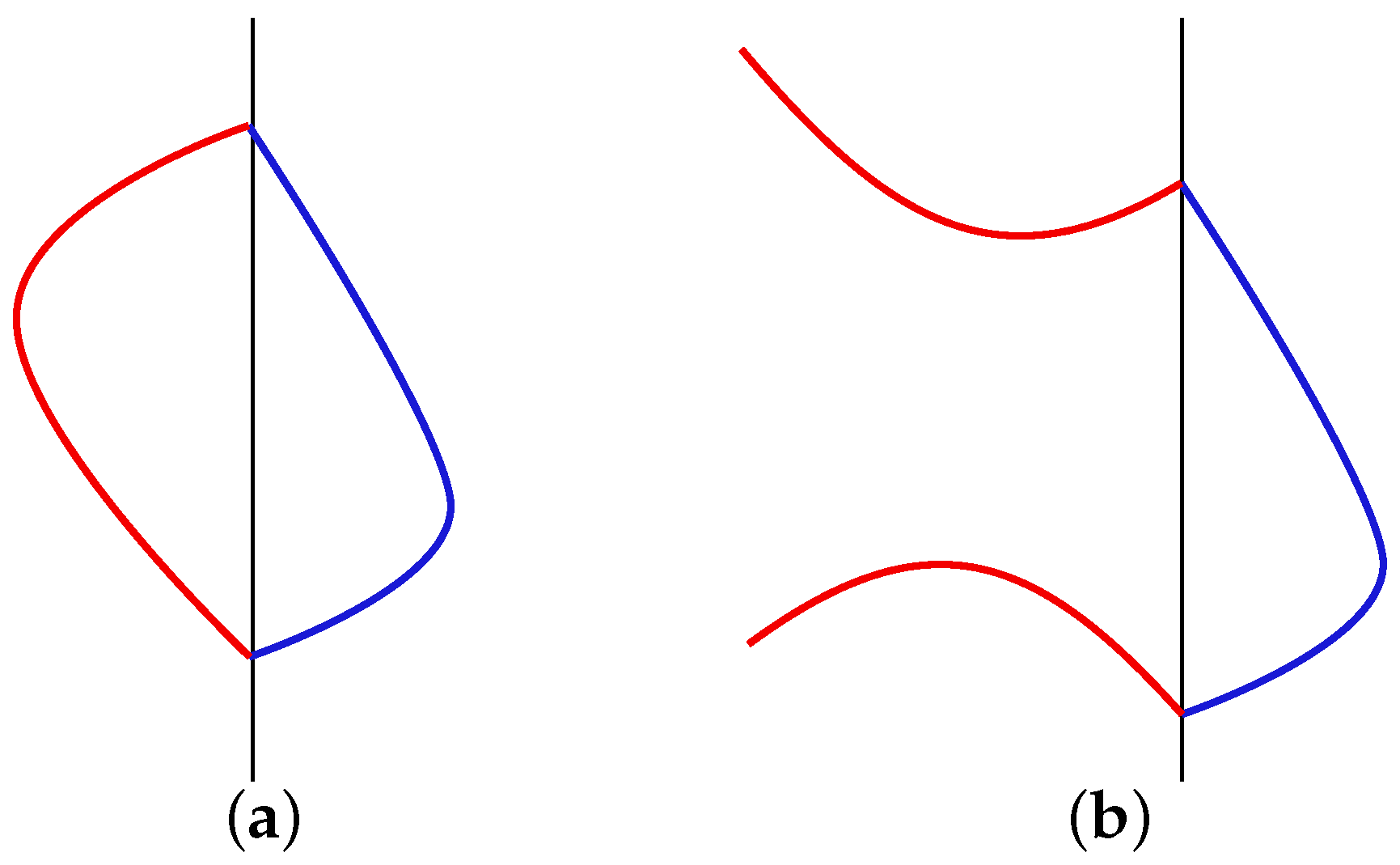
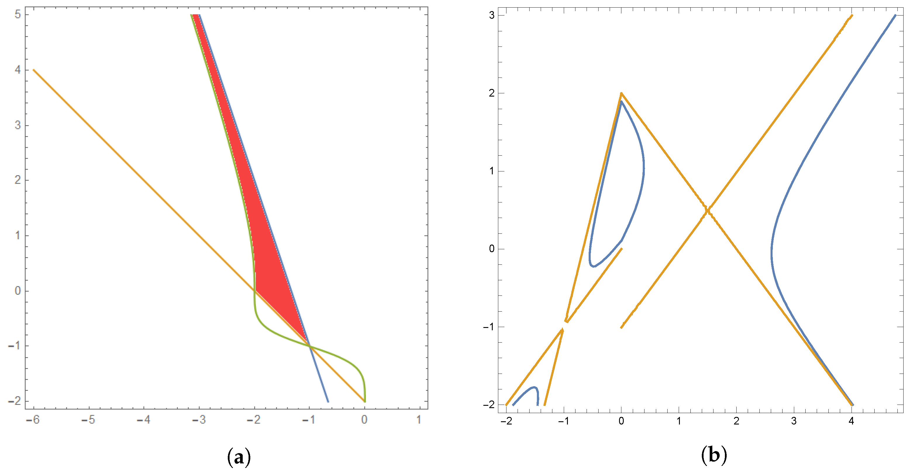
Hence, if we count the pairs of solutions $(y,Y)$ we can give an upper bound to the number of limit cycles of a piecewise differential system under the hypotheses of Theorem 2. However, this is only the upper bound because the connection between branches of the first integrals do not provide a closed curve, or a closed curve which, is not a periodic orbit, because the two pieces are not oriented in the same direction. Some examples of these phenomena can be seen in Figure 1.

Below these results are applied to the proof of Theorem 2.

Proposition 4.

Let γ be a limit cycle of a DPwLS (26) and (27) with a PFI on both sides of $\Sigma =\{x=0\}$. If one of the first integrals corresponds to a linear differential system with a saddle, γ intersects Σ at two points located between the two points of Σ, which belong to the separatrices of the saddle.

Proof. 

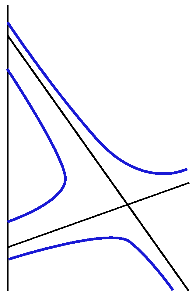
As a linear differential system, without common factors and having a PFI, it is topologically equivalent to a linear Hamiltonian system (see Proposition C in [14]), the $\omega$ and $\alpha$-limits of the orbits in the saddle case are restricted to the limits of the separatrices. Hence, any orbit out of its separatrices and far from the equilibrium point has a similar behavior to those which are two straight lines, according to Corollary 2. This implies that any orbit will cross $\Sigma$ twice if and only if both separatrices cross $\Sigma$ and the orbit is located at the hyperbolic region between the branches of the separatrices crossing $\Sigma$. See Figure 2. □

Lemma 1.

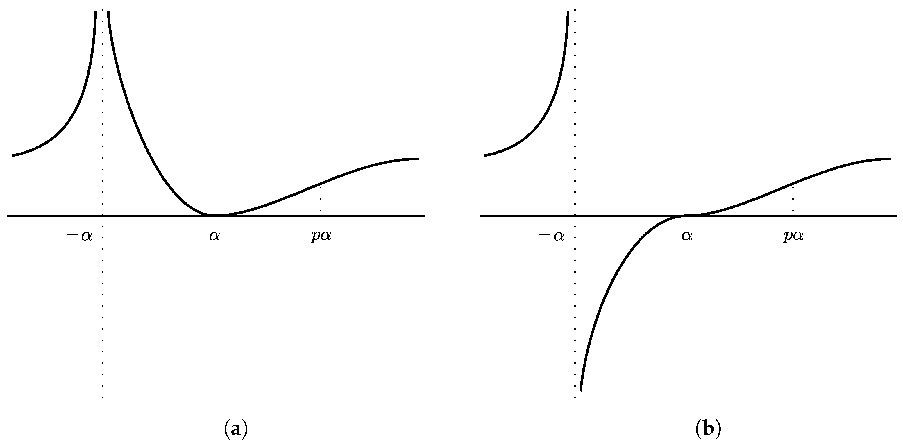
We consider the function $f_{p,\alpha }\left(x\right)={\left({\displaystyle \frac{x-\alpha }{x+\alpha }}\right)}^p$ for all $x\in \mathbb{R}\setminus \{-\alpha \}$ with $0<\alpha$ and $p\in {\mathbb{Z}}^{+}$. Thus it is satisfied that $f_{p,\alpha }\left(\alpha \right)=0$, $f_{p,\alpha }\left(0\right)={(-1)}^p$, $\underset{x\to \pm \infty }{lim}{f}_{p,\alpha }\left(x\right)=1$ and

(i) 

if p is even, $f_{p,\alpha }\left(x\right)>0$ for all $x\in \mathbb{R}\setminus \{-\alpha ,\alpha \}$, $f_{p,\alpha }$ decreases for $x\in (-\alpha ,\alpha )$ and increases outside, with a local minimum at $x=\alpha$ and an inflexion point at $x=p\alpha$; and,

(ii) 

if p is odd, $f_{p,\alpha }\left(x\right)>0$ if and only if $x\in \mathbb{R}\setminus (-\alpha ,\alpha )$, $f_{p,\alpha }$ increases for all $x\in \mathbb{R}\setminus \{-\alpha \}$, with an inflexion point at $x=\alpha$ and, if $p>1$, another one at $x=p\alpha$.

Proof. 

First, straightforward computations show that $f_{p,\alpha }\left(\alpha \right)=0$ and $f_{p,\alpha }\left(0\right)={(-1)}^p$.

Since

$$f_{p,\alpha }^{\prime }\left(x\right)=p{\left(\frac{x-\alpha }{x+\alpha }\right)}^{p-1}\frac{x+\alpha -x+\alpha }{{(x+\alpha )}^2}=\frac{2p\alpha }{{(x+\alpha )}^2}{\left(\frac{x-\alpha }{x+\alpha }\right)}^{p-1}.$$

Multiplying both sides by $(x-\alpha )(x+\alpha )$ gives

$$(x-\alpha )(x+\alpha )f_{p,\alpha }^{\prime }\left(x\right)=2p\alpha f_{p,\alpha }\left(x\right).$$

(34)

The second derivative is computed as

$$(x+\alpha +x-\alpha )f_{p,\alpha }^{\prime }\left(x\right)+(x-\alpha )(x+\alpha )f_{p,\alpha }^{″}\left(x\right)=2p\alpha f_{p,\alpha }^{\prime }\left(x\right),$$

then

$$2(x-p\alpha )f_{p,\alpha }^{\prime }\left(x\right)+(x-\alpha )(x+\alpha )f_{p,\alpha }^{″}\left(x\right)=0.$$

(35)

From (34), we conclude that if $f_{p,\alpha }^{\prime }\left(x\right)=0$ then also $f_{p,\alpha }\left(x\right)=0$. So, $x=\alpha$ is the only possible relative extreme. From (35), we conclude that $f_{p,\alpha }^{″}\left(x\right)=0$ if and only if $f_{p,\alpha }^{\prime }\left(x\right)=0$ or $2(x-p\alpha )=0$. Hence, there are two possible inflexion points, $x=\alpha$ and $x=p\alpha$.

(i)

When p is even, it is obvious that $f_{p,\alpha }\left(x\right)>0$ for all $x\in \mathbb{R}\setminus \{-\alpha ,\alpha \}$ and $f_{p,\alpha }\left(\alpha \right)=0$. From (34)

$$(x-\alpha )(x+\alpha )f_{p,\alpha }^{\prime }\left(x\right)>0,$$

which implies that either $(x-\alpha )(x+\alpha )>0$ and $f_{p,\alpha }^{\prime }\left(x\right)>0$, or $(x-\alpha )(x+\alpha )<0$ and $f_{p,\alpha }^{\prime }\left(x\right)<0$. Thus,

$$f_{p,\alpha }^{\prime }\left(x\right)>0\mathrm{if}x\in (-\infty ,-\alpha )\cup (\alpha ,\infty )$$

and

$$f_{p,\alpha }^{\prime }\left(x\right)<0\mathrm{if}x\in (-\alpha ,\alpha ).$$

Moreover, the sign of $f_{p,\alpha }^{\prime }\left(x\right)$ changes at $x=\alpha$. It is negative before $\alpha$ and positive after it, so at this point $f_{p,\alpha }$ has a local minimum.

Since $(x-\alpha )(x+\alpha )f_{p,\alpha }^{\prime }\left(x\right)>0$ is equivalent to $\frac{f_{p,\alpha }^{\prime }\left(x\right)}{(x-\alpha )(x+\alpha )}>0$, then (35) can be rewritten as

$$f_{p,\alpha }^{″}\left(x\right)=\frac{-f_{p,\alpha }^{\prime }\left(x\right)}{(x-\alpha )(x+\alpha )}2(x-p\alpha ),$$

hence, $f_{p,\alpha }^{″}\left(x\right)>0$ if and only if $2(x-p\alpha )<0$ or, equivalently, if $x<p\alpha$. This means that $f_{p,\alpha }$ has an inflexion point at $x=p\alpha$.

(ii)

When p is odd, $f_{p,\alpha }\left(x\right)$ is positive if and only if $(x-\alpha )(x+\alpha )>0$, i.e., $x\in (-\infty ,-\alpha )\cup (\alpha ,\infty )$. This implies that $f_{p,\alpha }\left(x\right)<0$ if and only if $x\in (-\alpha ,\alpha )$.

In order to study the monotonicity, (34) is used:

$$f_{p,\alpha }^{\prime }\left(x\right)=2p\alpha \frac{f_{p,\alpha }\left(x\right)}{(x-\alpha )(x+\alpha )}.$$

This implies that $\frac{f_{p,\alpha }\left(x\right)}{(x-\alpha )(x+\alpha )}>0$ for all $x\in \mathbb{R}\setminus \{-\alpha ,\alpha \}$. Since $\alpha >0$ we conclude that $f_{p,\alpha }^{\prime }\left(x\right)>0$ for all $x\in \mathbb{R}\setminus \{-\alpha ,\alpha \}$. So $f_{p,\alpha }$ is an increasing function in the whole domain.

Finally, we use (35) to study the convexity,

$$f_{p,\alpha }^{″}\left(x\right)=\frac{-f_{p,\alpha }^{\prime }\left(x\right)}{(x-\alpha )(x+\alpha )}2(x-p\alpha ).$$

As far as $f_{p,\alpha }^{\prime }\left(x\right)>0$ for all x, $f_{p,\alpha }^{″}\left(x\right)>0$ for $(x-\alpha )(x+\alpha )>0$ and $2(x-p\alpha )>0$, or $(x-\alpha )(x+\alpha )<0$ and $2(x-p\alpha )<0$. In the first case, if $x\in (-\infty ,-\alpha )\cup (\alpha ,\infty )$ and $x<p\alpha$, then $f_{p,\alpha }^{″}\left(x\right)>0$ if $x\in (-\infty ,-\alpha )\cup (\alpha ,p\alpha )$. In the second case, $f_{p,\alpha }^{″}\left(x\right)>0$ if $x\in (-\alpha ,\alpha )$ and $x>p\alpha$. However, $p\alpha \ge \alpha$, and since $p\in {\mathbb{Z}}^{+}$ and $\alpha >0$, then there is no other solution for x where $f_{p,\alpha }^{″}\left(x\right)>0$. In conclusion, $f_{p,\alpha }^{″}\left(x\right)>0$ if and only if $x\in (-\infty ,-\alpha )\cup (\alpha ,p\alpha )$. In a similar way, we conclude that $f_{p,\alpha }^{″}\left(x\right)<0$ if, and only if, $x\in (-\alpha ,\alpha )\cup (p\alpha ,\infty )$.

Thus, the proof is complete. □

Remark 3.

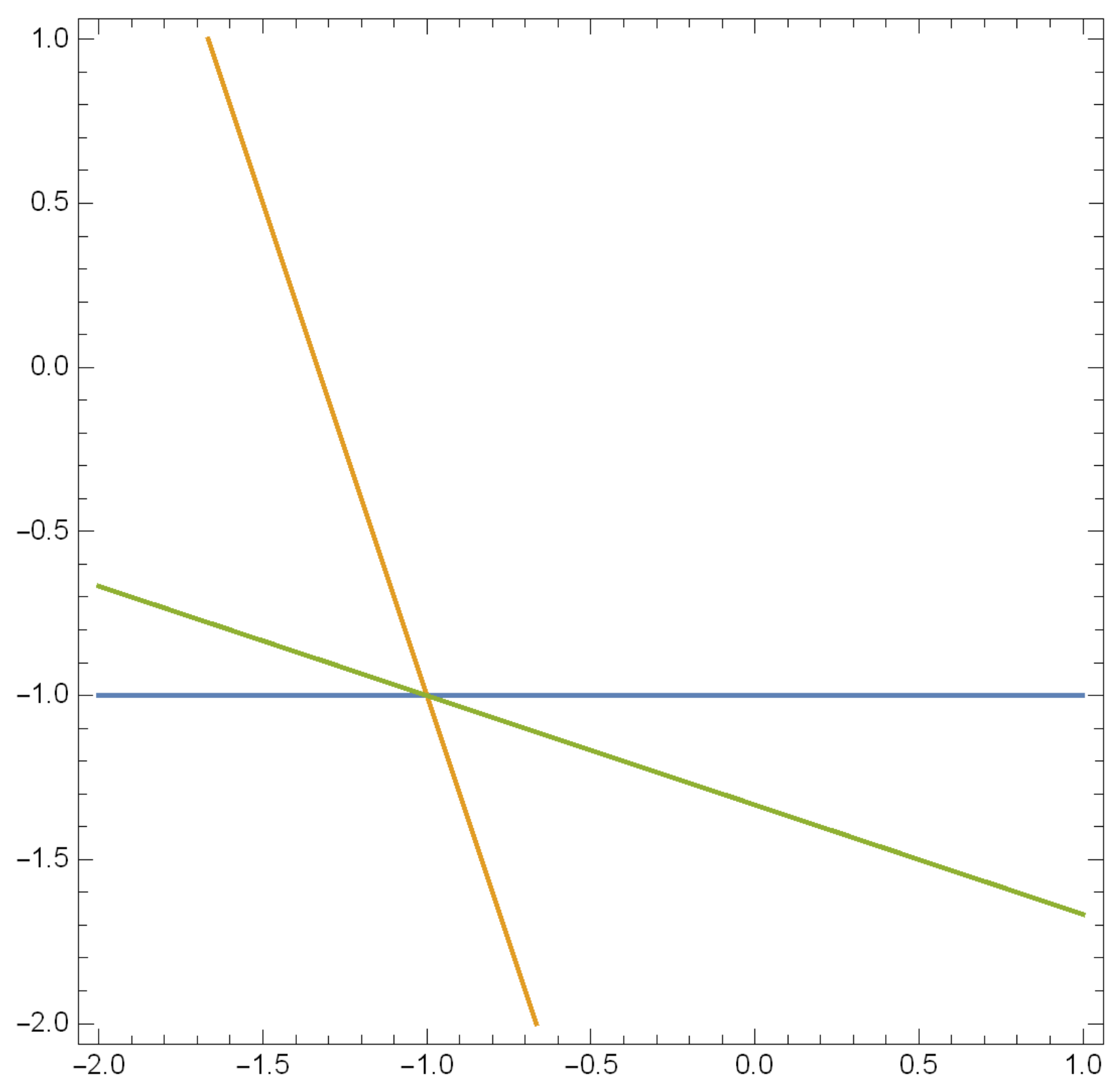
Figure 3 shows graphical representations of the results obtained in this proof.

Proof of Theorem 2.

Taking into account Corollary 2, it is enough to check Theorem 2 for the planar DPwLS (26) and (27). We divide the proof into three cases according to Corollary 2, which controls when the linear differential systems (26) and (27) have PFI.

• Case 1: Systems (26) and (27) are both Hamiltonian. Therefore, from Proposition 3 in system (27), $r=0$. Similarly, in system (26), $\ell =0$. In this case, every limit cycle of DPwLS (26) and (27) crosses $x=0$ at two different points $(0,y)$ and $(0,Y)$, satisfying the system

  $$\begin{array}{c}{e}_1={\widehat{H}}_1(0,y)-{\widehat{H}}_1(0,Y)=(y-Y)(y+Y)=0,\hfill \\ e_2={\widehat{H}}_3(0,y)-{\widehat{H}}_3(0,Y)=(y-Y)(y+Y-2j)=0,\hfill \end{array}$$

  using the notation of Corollary 2.

We are only interested in the solutions in which $y\ne Y$. System $e_1=0$, $e_2=0$ either has no solutions, or has an infinite number of solutions when $j=0$. Consequently, there are no isolated solutions, and therefore, in this case, the DPwLS (26) and (27) have no limit cycles.

• Case 2: Only system (26) is Hamiltonian. From Proposition 3, system (27) has $\beta =1$ and $r={\displaystyle \frac{q-p}{q+p}}\ne 0$ with $p,q\in {\mathbb{Z}}^{+}$, and system (26) has $\ell =0$. In this case, every limit cycle of the DPwLS (26) and (27) crosses $x=0$ at two different points $(0,y)$ and $(0,Y)$ satisfying the system

  $$\begin{array}{cc}\hfill e_1=& {\widehat{H}}_1(0,y)-{\widehat{H}}_1(0,Y)=(y-Y)(y+Y)=0,\hfill \\ \hfill e_2=& {\widehat{H}}_4(0,y)-{\widehat{H}}_4(0,Y)\hfill \\ \hfill =& {\left(y+{\displaystyle \frac{k(q+p)}{2q}}-j\right)}^p{\left(y-{\displaystyle \frac{k(q+p)}{2p}}-j\right)}^q-\hfill \\ & {\left(Y+{\displaystyle \frac{k(q+p)}{2q}}-j\right)}^p{\left(Y-{\displaystyle \frac{k(q+p)}{2p}}-j\right)}^q=0.\hfill \end{array}$$

As in the previous case, we are only interested in solutions in which $y\ne Y$. As $e_1=0$ implies that $y=-Y$, $e_2=0$ implies that

$$\begin{array}{cc}& {\left(-Y+{\displaystyle \frac{k(q+p)}{2q}}-j\right)}^p{\left(-Y-{\displaystyle \frac{k(q+p)}{2p}}-j\right)}^q\hfill \\ & ={\left(Y+{\displaystyle \frac{k(q+p)}{2q}}-j\right)}^p{\left(Y-{\displaystyle \frac{k(q+p)}{2p}}-j\right)}^q,\hfill \end{array}$$

or, equivalently

$${\left(\frac{-Y+{\displaystyle \frac{k(q+p)}{2q}}-j}{Y+{\displaystyle \frac{k(q+p)}{2q}}-j}\right)}^p={\left(\frac{Y-{\displaystyle \frac{k(q+p)}{2p}}-j}{-Y-{\displaystyle \frac{k(q+p)}{2p}}-j}\right)}^q.$$

Lemma 1 gives the need for:

$$f_{p,\alpha }\left(Y\right)={(-1)}^{p+q}{f}_{q,\beta }\left(Y\right),$$

where $\alpha =\frac{k(p+q)}{2q}-j$ and $\beta =j+\frac{k(p+q)}{2p}$. We can assume k is positive, otherwise switching $\overline{k}=-k>0$, $\overline{p}=q$ and $\overline{q}=p$ will expand the same equation, $e_2=0$, under this assumption. In this case, $-\alpha <j<\beta$ and according to Proposition 4, we should look for solutions $Y\in (-\alpha ,\beta )$. Furthermore, as $y=-Y$, there is a solution in $(-\alpha ,\beta )$, which implies that $(-|Y|,|Y\left|\right)\subset (-\alpha ,\beta )$, so $\alpha$ and $\beta$ are both positive.

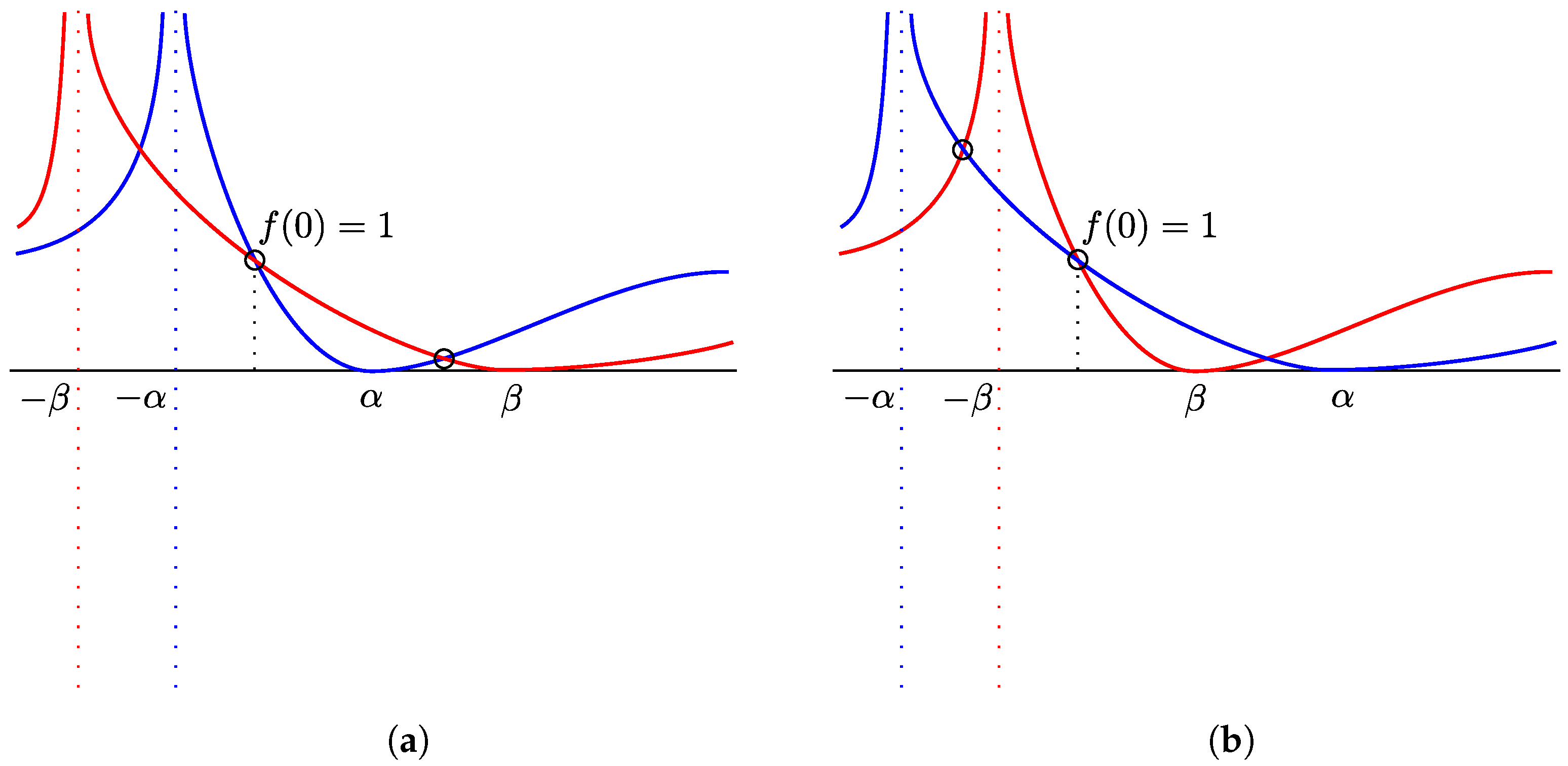
The proof is completed by showing that the graphs of $f_{p,\alpha }\left(x\right)$ and ${(-1)}^{p+q}{f}_{q,\beta }\left(x\right)$ cut each other in one non-vanishing value of $x\in (-\alpha ,\beta )$, at most. In order to check this, we must take into account the parity of p and q and the relative positions of $\alpha$ and $\beta$. Lemma 1 is the key to this analysis.

Nevertheless, we only need to consider one case: p and q even. In Statements (ii) and (iii) of Theorem 1, without loss of generality, we can assume that p and q are both even. On the contrary, $p^{\prime }=2p$ and $q^{\prime }=2q$ are both even, satisfying the same hypotheses of the theorem for the same differential system and giving a PFI, $H_j^{\prime }$, such that $H_j^{\prime }={\left(H_j\right)}^2$ for any $j=2,3$.

Let p and q be even integers. In this case, ${(-1)}^{p+q}=1$, so we will compare $f_{p,\alpha }$ and $f_{q,\beta }$. For $\alpha <\beta$, we divide $(-\alpha ,\beta )$, studying intervals $(-\alpha ,\alpha )$ and $(\alpha ,\beta )$ separately. At both intervals, $f_{p,\alpha }$ and $f_{q,\beta }$ are positive functions. However, at $(-\alpha ,\alpha )$, both functions decreases while at $(\alpha ,\beta )$$f_{p,\alpha }$ increases and $f_{q,\beta }$ decreases. Since 0 belongs to $(-\alpha ,\alpha )$ and both functions have the same value at this point, 1, there are no inflexion points in this interval. There are no other points in common between the two graphs in this interval. In interval $(\alpha ,\beta )$, the monotonicity is enough to assure the existence of a point in common because $f_{p,\alpha }\left(\alpha \right)=0$, $f_{p,\alpha }\left(\beta \right)>0$, $f_{q,\beta }\left(\alpha \right)>0$ and $f_{q,\beta }\left(\beta \right)=0$. Figure 4 summarizes our proof.

If $\beta <\alpha$, similar arguments can be developed, but analyzing the functions at the intervals $(-\alpha ,-\beta )$ and $(-\beta ,\beta )$ separately. This completes the desired conclusion, with at most one limit cycle.

• Case 3: Only system (27) is Hamiltonian. Again, from Proposition 3, in system (27) $r=0$ and in system (26) $\alpha =1$ and $\ell =\frac{q-p}{q+p}\ne 0$ with $p,q\in {\mathbb{Z}}^{+}$. In this case, every limit cycle of the DPwLS (26) and (27) crosses $x=0$ at two different points, $(0,y)$ and $(0,Y)$, satisfying the system

  $$\begin{array}{cc}\hfill e_1=& {\widehat{H}}_2(0,y)-{\widehat{H}}_2(0,Y)\hfill \\ \hfill =& {\left(y+{\displaystyle \frac{g(q+p)}{2q}}\right)}^p{\left(y-{\displaystyle \frac{g(q+p)}{2p}}\right)}^q-{\left(Y+{\displaystyle \frac{g(q+p)}{2q}}\right)}^p{\left(Y-{\displaystyle \frac{g(q+p)}{2p}}\right)}^q=0.\hfill \\ \hfill e_2=& {\widehat{H}}_3(0,y)-{\widehat{H}}_3(0,Y)=(y-Y)(y+Y)=0,\hfill \end{array}$$

  Similar arguments as the ones used in Case 2 show that DPwLS (26) and (27) have at most one limit cycle.

Therefore, we have completed the proof of Theorem 2. □

4. Examples

In this section, we show that the bound obtained in Theorem 2 can be achieved. We consider $A^{-}=\left(\begin{array}{cc}2& -1\\ 3& -2\end{array}\right)$, $A^{+}=\left(\begin{array}{cc}1/2& 1\\ 1& 1/2\end{array}\right)$, $b^{-}=\left(\begin{array}{c}1\\ 1\end{array}\right)$ and $b^{+}=\left(\begin{array}{c}a\\ d\end{array}\right)$ with $a,d\in \mathbb{R}$ and the piecewise linear system given by

$$\left(\begin{array}{c}\dot{x}\\ \dot{y}\end{array}\right)=A^{-}\left(\begin{array}{c}x\\ y\end{array}\right)+b^{-},$$

(36)

if $x\le 0$, and

$$\left(\begin{array}{c}\dot{x}\\ \dot{y}\end{array}\right)=A^{+}\left(\begin{array}{c}x\\ y\end{array}\right)+b^{+},$$

(37)

if $x\ge 0$.

System (36) satisfies the hypotheses of Theorem 1 statement (i). It means that System (36) is a Hamiltonian system and has $H^{-}=3x^2+y^2-4xy+2x-2y$ as a first integral. Moreover, this system has a saddle located at $(-1,-1)$ and its separatrices are $y=x$ (unstable) and $y=3x+2$ (stable). These separatrices cut the vertical axis at $(0,0)$ and $(0,2)$.

System (37) satisfies the hypotheses of Theorem 1 statement (ii) with $p=1$ and $q=3$. Thus, system (37) has the PFI

$$H^{+}=\left(y+x+\frac{2}{3}(a+d)\right){\left(y-x+2(a-d)\right)}^3.$$

This shows that this system has a saddle located at $\left(\frac{2a-4d}{3},\frac{2d-4a}{3}\right)$ and its separatrices are $y=-x-\frac{2}{3}(a+d)$ (stable) and $y=x-2(a-d)$ (unstable). These separatrices cut the vertical axis at $(0,-\frac{2}{3}(a+d))$ and $(0,-2(a-d\left)\right)$.

We denote $\gamma =\frac{2}{3}(a+d)$ and $\theta =2(a-d)$. In this way, as mentioned before, we can characterize the limit cycles solving system

$$\begin{array}{c}{H}^{+}(0,y_1)-H^{+}(0,y_0)=0,\hfill \\ H^{-}(0,y_1)-H^{-}(0,y_0)=0,\hfill \end{array}$$

(38)

where $y_1$ and $y_0$ are unknown and identify points at ${\Sigma }_0=\{(x,y)\in {\mathbb{R}}^2:x=0\}$ that characterize both level curves completing the cycle, if one exists. If we compute the resultant of both left-hand side expressions with respect to $y_1$, we conclude that, in order to have a limit cycle, a necessary condition is that $y_0$ satisfies the equation

$$R\left(y_0\right)=-(4+\gamma +3\theta )y_0^2+2(4+\gamma +3\theta )y_0-{\theta }^3-3\gamma {\theta }^2-6{\theta }^2-6\gamma \theta -12\theta -4\gamma -8=0.$$

The discriminant of this quadratic equation is

$$D(\gamma ,\theta )=-4{(1+\theta )}^2(4+3\gamma +\theta )(4+\gamma +3\theta ).$$

Figure 5 shows the set of points where $D(\gamma ,\theta )$ vanishes. Thus, these straight lines bound the regions where the discriminant does not vanish and $R\left(y_0\right)=0$ may or may not have real solutions.

As $(0,y_0)$ is an intersection point of the limit cycle with ${\Sigma }_0$ and any limit cycle requires two of these points, we look for the region where $R\left(y_0\right)=0$ has two real different solutions. This means that we are interested in $D(\gamma ,\theta )>0$, or equivalently,

$$(4+3\gamma +\theta )(4+\gamma +3\theta )<0.$$

In order to assure the existence of a limit cycle, the solutions of $R\left(y_0\right)=0$ must be located at $(-2,0)$ and between $-\gamma$ and $-\theta$, the intersection points of the separatrices and ${\Sigma }_0$. The equations

$$\begin{array}{c}R(-\gamma )=-{(2+\gamma +\theta )}^3=0,\hfill \\ R(-\theta )=-4{(1+\theta )}^2(2+\gamma +\theta )=0,\hfill \\ R\left(0\right)=-8-4\gamma -12\theta -6\gamma \theta -6{\theta }^2-3\gamma {\theta }^2-{\theta }^3=0,\hfill \\ R(-2)=-40-12\gamma -36\theta -6\gamma \theta -6{\theta }^2-3\gamma {\theta }^2-{\theta }^3=0\hfill \end{array}$$

characterize the regions that must be studied. It is simple to check that we have found algebraic limit cycles if $\gamma$ and $\theta$ satisfy

$$\begin{array}{c}2+\gamma +\theta >0,\hfill \\ 4+3\gamma +\theta <0,\hfill \\ -8-4\gamma -12\theta -6\gamma \theta -6{\theta }^2-3\gamma {\theta }^2-{\theta }^3<0.\hfill \end{array}$$

Figure 6 shows the region described above, as well as the limit cycle found for $\gamma =-2$ and $\theta =1$. In this case, we see that the limit cycle passes through the points $(0,1-\frac{2\sqrt{5}}{5})\approx (0,0.105573)$ and $(0,1+\frac{2\sqrt{5}}{5})\approx (0,1.89443)$.

5. Discussion

We have illustrated how to study the limit cycles of piecewise differential systems separated by one straight line and formed by two integrable systems. Here, we have considered that the first integrals of both differential systems are polynomials with one of the differential systems being a Hamiltonian system, and consequently, if the piecewise differential system has limit cycles, these are algebraic. Under this assumption, the piecewise differential system has no more than one limit cycle. Additionally, we have characterized the linear differential systems with polynomial first integrals.

References

- Filippov, A.F. Differential Equations with Discontinuous Right–Hand Sides; Mathematics and Its Applications (Soviet Series); Translated from Russian; Kluwer Academic Publishers Group: Dordrecht, The Netherlands, 1988; Volume 18. [Google Scholar]
- Andronov, A.; Vitt, A.; Khaikin, S. Theory of Oscillations; Pergamon Press: Oxford, UK, 1966. [Google Scholar]
- Di Bernardo, M.; Budd, C.J.; Champneys, A.R.; Kowalczyk, P. Piecewise-Smooth Dynamical Systems: Theory and Applications; Springer: London, UK, 2008; Volume 163. [Google Scholar]
- Simpson, D.J.W. Bifurcations in Piecewise-Smooth Continuous Systems; World Scientific: Singapore, 2010. [Google Scholar]
- Makarenko, O.; Lamb, J.S.W. Dynamics and bifurcations of nonsmooth systems: A survey. Physica D 2012, 241, 1826–1844. [Google Scholar]
- Euzébio, R.D.; Llibre, J. On the number of limit cycles in discontinuous piecewise linear differential systems with two pieces separated by a straight line. J. Math. Anal. Appl. 2015, 424, 475–486. [Google Scholar] [CrossRef] [Green Version]
- Buzzi, C.; Gasull, A.; Torregrosa, J. Algebraic limit cycles in piecewise linear differential systems. Int. J. Bifurc. Chaos 2018, 28, 1850039. [Google Scholar] [CrossRef]
- Artés, J.C.; Llibre, J.; Vulpe, N. Quadratic systems with an integrable saddle: A complete classification in the coefficient space R12. Nonlinear Anal. 2012, 75, 5416–5447. [Google Scholar] [CrossRef] [Green Version]
- Li, T.; Llibre, J. Limit cycles in piecewise polynomial Hamiltonian systems allowing nonlinear switching boundaries. J. Differ. Equ. 2023, 344, 405–438. [Google Scholar] [CrossRef]
- Dieci, L.; Elia, C.; Pi, D. Limit cycles for regularized discontinuous dynamical systems with a hyperplane of discontinuity. Discret. Contin. Dyn. Syst. B 2017, 22, 3091–3112. [Google Scholar] [CrossRef] [Green Version]
- Huzak, R.; Uldall Kristiansen, K. The number of limit cycles for regularized piecewise polynomial systems is unbounded. J. Differ. Equ. 2023, 342, 34–62. [Google Scholar] [CrossRef]
- Sotomayor, J.; Teixeira, M.A. Regularization of discontinuous vector fields. In Proceedings of the International Conference on Differential Equations, Lisboa, Portugal, 24–29 July 1995; pp. 207–223. [Google Scholar]
- Freire, E.; Ponce, E.; Torres, F. Canonical Discontinuous Planar Piecewise Linear Systems. SIAM J. Appl. Dyn. Syst. 2012, 11, 181–211. [Google Scholar] [CrossRef]
- García, B.; Llibre, J.; Pérez del Río, J.S. Phase portraits of the quadratic vector fields with a polynomial first integral. Rend. Circ. Mat. Palermo 2006, 55, 420–440. [Google Scholar] [CrossRef]
Figure 1.
Some possible connections between both side branches. (a) Cycle shape appears; (b) It is not a cycle.
Figure 2.
Graphical representation of a polynomial saddle phase portrait.
Figure 3.
Graphical representations of from Lemma 1. (a) p is even; (b) p is odd.
Figure 4.
p and q even. (a) ; (b) .
Figure 5.
Regions delimited by .
Figure 6.
(a) Region with limit cycle; (b) Limit cycle found for and .
Disclaimer/Publisher’s Note: The statements, opinions and data contained in all publications are solely those of the individual author(s) and contributor(s) and not of MDPI and/or the editor(s). MDPI and/or the editor(s) disclaim responsibility for any injury to people or property resulting from any ideas, methods, instructions or products referred to in the content. |
© 2023 by the authors. Licensee MDPI, Basel, Switzerland. This article is an open access article distributed under the terms and conditions of the Creative Commons Attribution (CC BY) license (https://creativecommons.org/licenses/by/4.0/).
Share and Cite
MDPI and ACS Style
García, B.; Llibre, J.; Pérez del Río, J.S.; Pérez-González, S. Limit Cycles of Polynomially Integrable Piecewise Differential Systems. Axioms 2023, 12, 342. https://doi.org/10.3390/axioms12040342
AMA Style
García B, Llibre J, Pérez del Río JS, Pérez-González S. Limit Cycles of Polynomially Integrable Piecewise Differential Systems. Axioms. 2023; 12(4):342. https://doi.org/10.3390/axioms12040342
Chicago/Turabian StyleGarcía, Belén, Jaume Llibre, Jesús S. Pérez del Río, and Set Pérez-González. 2023. "Limit Cycles of Polynomially Integrable Piecewise Differential Systems" Axioms 12, no. 4: 342. https://doi.org/10.3390/axioms12040342
Note that from the first issue of 2016, this journal uses article numbers instead of page numbers. See further details here.