
Incorporating Stochastic Wind Vectors in Wildfire Spread Prediction

School of Science, University of New South Wales, Canberra, ACT 2612, Australia
*
Author to whom correspondence should be addressed.
Atmosphere 2023, 14(11), 1609; https://doi.org/10.3390/atmos14111609
Submission received: 22 August 2023
/
Revised: 12 October 2023
/
Accepted: 24 October 2023
/
Published: 27 October 2023
(This article belongs to the Special Issue Wildfires Modeling: Recent Trends, Current Progress and Future Directions)
Abstract
:The stochastic nature of environmental factors that govern the behavior of fire, such as wind and fuel, exposes wildfire modeling to a degree of uncertainty. In order to produce more realistic wildfire predictions, it is, therefore, necessary to incorporate these uncertainties within wildfire models in a way that reflects the influence of environmental stochasticity on wildfire propagation. Otherwise, the risks of the potential danger of a given wildfire may be under-represented. Specifically, environmental stochasticity in the form of wind variability results in considerable uncertainty in the output of fire spread models. Here, we consider two stochastic wind models and their implementation in the spark fire simulator framework to capture the environmental uncertainty related to wind variability. The results are compared with the output from purely deterministic wildfire spread models and are discussed in the context of the potential ramifications for wildfire risk management.
1. Introduction
Wildland fires are a naturally occurring phenomenon, the impacts of which can be exacerbated or ameliorated by human actions. Fire plays an essential role in many ecosystems, but when not adequately managed, it can have disastrous impacts on natural systems and human lives and assets. Indeed, many of the wildland fires that have occurred around the world over the last two decades constitute significant natural disasters, particularly in regions such as southeastern Australia and western North America [1,2,3]. Anthropogenic climate change is also affecting fire occurrence and severity around the globe and is a likely driver of the increase in the frequency of very large and destructive wildland fires that have been observed [4,5,6]. The Black Summer fires that occurred during 2019–2020 over southeastern Australia serve as a particularly telling example. These fires burnt over the course of several months and directly caused 33 deaths, including 26 civilians and seven firefighters [7]. Extensive smoke from the fires resulted in almost 450 additional deaths due to smoke inhalation and affected around 80% of the population [8,9]. It is further estimated that in excess of one billion animals perished in the fires [10].
Wildfire management, which encompasses risk assessment and decision-making, ecological considerations, strategic fuel management, and fire suppression (direct or indirect), has an important role to play in mitigating wildfire impact. It requires considerable resources, which need to be deployed in a cost-effective manner. Wildfire spread prediction is critical in supporting decision-making related to the deployment of resources, suppression tactics, the issuance of public evacuation orders, and other aspects of wildfire management and emergency response.
Mathematical models of wildfire spread have been developed to predict fire behavior since the 1940s [11]. There are different types of fire behavior models, including empirical and semi-empirical models, such as artificial intelligent (AI) models, which are based on experiments and historical data, and physics-based models that are based on physical and mathematical relationships between inputs and the rate of fire spread [12]. Because of their computational simplicity, empirical models are usually preferred [13] in most operational systems, and for this reason, empirical models are used in this study for developing the rate of fire spread.
Two-dimensional empirical and semi-empirical fire propagation models were established based on an anisotropic Huygens principle [14]. These models typically require weather inputs such as wind, temperature, relative humidity, and the moisture content of the fuel, as well as fuel and topographic conditions. Fire propagation is particularly sensitive to variations in wind speed and direction [15]. The rate of fire propagation is approximately proportional to the square of wind speed (when >) [16]. This effect can be further increased under certain conditions, such as when fuel moisture content is low. As such, spatial and temporal variations in wind inputs can have significant impacts on the propagation of a fire [17,18]. Spatio-temporal variation in the wind field, along with variations in the other driving factors, can cause a considerable range of uncertainty in the prediction of fire spread, so much so that it is considered routine for actual fire spread to differ from the predicted fire spread by a factor of ±30% [19]. Therefore, the inclusion of wind models that account for the intrinsic uncertainty of the wind field and understanding how they might influence the output of operational fire propagation models represent important aspects of effective fire risk management [20,21].
In order to better accommodate the influence of the spatial and temporal variability of weather-related factors in fire spread prediction, modelers have pursued various probabilistic approaches. In one approach, which is here referred to as the “deterministic ensemble” approach, weather inputs are repeatedly sampled from a particular probability distribution. Each of the sampled input datasets is then applied in a deterministic fire-spread model, providing an ensemble of possible fire-spread outcomes. In the most basic implementations of the deterministic ensemble approach, fire weather inputs are sampled from standard probability distributions, such as the uniform distribution (e.g., Fireds [22]) or the normal distribution (e.g., spark [23]), whereas in more sophisticated implementations, the forecast and historical data are combined to produce a more faithful statistical characterization of weather inputs at a particular location (e.g., wfdss [24]). This deterministic ensemble approach was also applied in the context of one-dimensional rate-of-spread prediction by [25], who sampled input conditions from a normal distribution but also noted the potential use of the Weibull distribution for sampling wind speed. Hilton et al. [26] and Dabrowski et al. [17] incorporated random components in a fire propagation model, which resulted in a probabilistic technique for predicting wildfire propagation.
Specifically, Hilton et al. [26] added the spatial and temporal variation of environmental factors, such as combustion condition, wind speed, and wind direction, to the rate of fire spread prediction based on the level set method. The variation in the elements was investigated by picking random values for the inputs from a Gaussian distribution with a prescribed standard deviation. The resultant simulations compared favorably with observed grassland fires, thus highlighting the potential improvements that such an approach could have in fire propagation modeling. The analyses carried out by [26] demonstrated that variation in the combustion condition slows the rate of fire growth and creates an irregular fire front, whereas wind variation produces more rounded flanks and alters the geometric shape of the fire perimeter for simulations initialized with a straight fire line. Although this study introduced some randomness to fire spread simulation, the simulations generated roughly symmetrical fire perimeters that did not show any indication of natural variability of wind over time, nor did it consider ensemble runs to assess the spatial variability of risk.
Although deterministic ensemble approaches, along with other probabilistic wildfire spread models, such as [26], account for variability in a wind field and other driving factors, they do not really acknowledge the inherent stochasticity of the wind vector, nor do they acknowledge the process-based nature of wind variability [27].
On the other hand, in other areas of study related to wind modeling, e.g., for wind energy applications and wind farms, the wind is explicitly treated as a stochastic variable [28]. Indeed, there have been several studies that have treated wind as a stochastic process. Bivona et al. [27] developed a class of stochastic models for an hourly averaged wind speed time series using the models of [29]. The proposed stochastic models were then evaluated for wind speed time series recorded in two regions in Italy over four years, and it was found that the results captured the wind speed distributions in of cases.
The Ornstein-Uhlenbeck (ou) process, also known as the “First-Order Gauss-Markov (fogm) process”, has been frequently utilized for wind modeling, especially in applications related to wind power generation. Arenas et al. [30] considered the relationship between mean wind speed and turbulence intensity using the ou process to capture wind speed variability, and wind magnitude and direction data at altitudes of up to 20 km were used by Turkoglu et al. [31] to calibrate an ou process model to better inform real-time guidance strategies in avionics applications. Their results showed that the wind simulations reasonably imitate the stochastic nature of the wind characteristics. Zarate et al. [32] applied the continuous format of stochastic differential equations (Wiener process) to generate wind speed profiles with statistical properties, including mean, variance, and autocorrelation. These profiles were constructed based on historical wind speed data for a specific location and were designed to be suitable for power system dynamic studies.
Benth et al. [33] investigated the correlation between electricity prices and wind power production in wind energy markets. Specifically, they modeled wind speed using the ou process and calibrated the parameters based on wind observations, with the practical intention of helping inform business strategy and risk assessment for energy producers. Loukatou et al. [28] also showed the advantage of a dynamic representation in continuous time for random wind speed variation through the application of the ou process.
Stochastic process models have also seen some limited use in bushfire modeling applications. For example, Zazali et al. [34] considered a basic deterministic bushfire model and incorporated stochasticity in the model by treating wind speed and direction as Wiener processes. They compared the resulting stochastic model with corresponding deterministic ensembles and demonstrated that the stochastic model generated a broader range of possible fire perimeters than the deterministic ensemble approach.
In the present study, we attempt to accommodate the environmental uncertainty that arises due to temporal variations in the wind vector in a wildfire spread model within the two-dimensional fire simulation platform spark [35], which models fire propagation using a level set-based approach [26]. We model the wind vector using two different stochastic processes, namely the Wiener process and the fogm process, using the wind observations of Quil et al. [20] to calibrate the required parameters. The stochastic wind models are then incorporated within the workflow of spark.
2. Data and Methodology
2.1. Wind Data
The parameters defining the stochastic process models used in this study were calibrated using two months of wind observations collected by Quil et al. [36] from a field site near Canberra Airport (35.28722 S, 149.17440 E). The data comprised wind speed and wind direction recorded every 5 min by 11 Davis 1 Vantage Pro 2TM Portable Automatic Weather Stations labeled paw1–paw11, which were situated in close proximity (i.e., within an area of approximately 20 m × 20 m). The data collection period spanned 57 days, from 14 February to 11 April 2014, except for the paw9 station, the data of which only covers the period 14–27 February 2014.
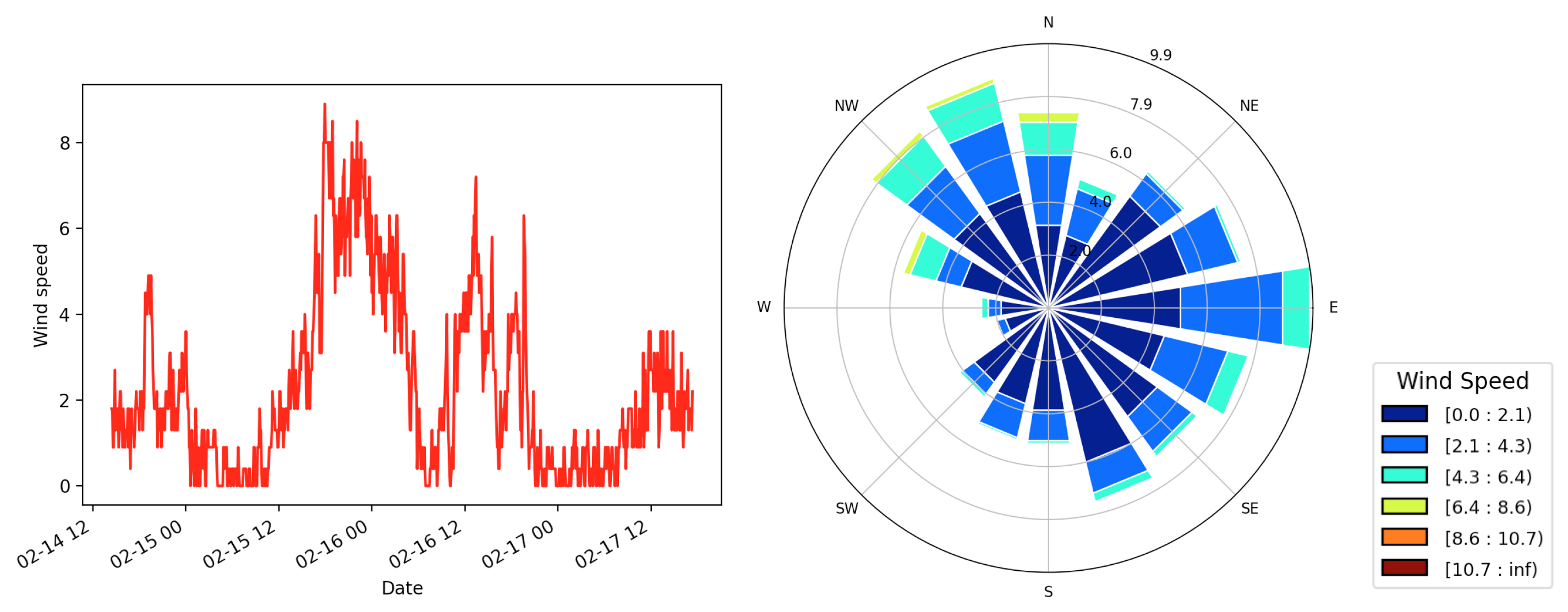
Figure 1 shows the variability in the observed wind speed and direction data over three days in February 2014. The wind speed varies between and overall and exhibits a considerable hourly variation of 2–4 , which highlights the importance of incorporating the variation of wind in fire simulations.
In this study, we consider wind speed and direction as stochastic processes. However, to prevent the generation of negative wind speeds during the simulation process and to avoid the difficulties of working with circular variables, we work with the components of the wind vector rather than wind speed and direction. The wind vector components are defined as follows:
where is the wind speed and is the wind direction. We adopt the convention that the x-component points in an easterly direction and the y-component points in a northerly direction.
2.2. Stochastic Models
Although the deterministic ensemble approach can potentially capture the uncertainties associated with fire modeling and, therefore, provide information more suited to risk management, it also has its limitations. Ensemble approaches ideally require a large number of ensemble members to support predictions that accurately cover the range of possible fire propagation scenarios. This can be achieved at a considerable computational expense, even for empirical models that can perform single runs much faster than in real time. Additionally, the probability distribution for a particular input parameter is not always known, and determining an appropriate candidate is not a trivial task. For example, the distribution of wind speed at a particular location may not necessarily fit a standard probability distribution, such as a normal distribution, and can depend on factors such as topographic setting [25,37]. Furthermore, the deterministic ensemble methodology fails to address the spatio-temporal fluctuations in environmental inputs. This approach is unable to sufficiently capture the dynamic and evolving nature of these inputs, as indicated by Zazali et al. [34]. Moreover, it does not incorporate the temporal autocorrelation present in environmental factors, such as the wind factor reported by Loukatou et al. [28].
For example, the Canadian Forest Fire Weather Index System (cffwis), which captures daily weather observations, was developed to represent such temporal auto-dependencies by a Markov Chain process [38]. In general, a Markov Chain process can be expressed mathematically as
Dabrowski et al. [17] added stochastic noise to wind inputs for the Rothermel model for rate-of-fire spread. The fire propagation contours were then predicted using a Bayesian approach, which resulted in promising outcomes in terms of introducing uncertainty into the spark fire simulator.
In the present study, two stochastic processes are considered as candidate models to estimate the variation in wind vector components over time: the discretized random walk and the fogm process. Not only have these stochastic processes attracted attention from modelers as a way to simulate environmental factors, but they have also been shown to produce simulations that are more appropriate to assessing risk when compared to deterministic predictions, even in areas outside the environmental sciences [39,40].
The random walk process has independent increments that are normally distributed for and the random variable , , where denotes a normally distributed random variable with zero mean and unit variance [41]. As another option for modeling the wind vector, the continuous version of the random walk is the Wiener process with infinitesimally small time steps, which inherits the same mathematical description as the random walk process [34].
In the random walk process, the wind vector at the current time can be determined from the previous state . The discretized first-order equation of the random walk can be represented as the following difference Equation (3) for the x and y components of the wind vector .
where and are the magnitudes of the process noise for the x and y components with a time step of , and is a Gaussian random variable with mean zero and variance 1.
In comparison, the fogm process is a mean-reverting and stationary process [31]. In this process, the current state wind vector can also be deduced from the previous state , as described by the first-order difference Equation (4) [42],
where and are the magnitude of the fogm process noise for the x and y components of the wind vector with a time step of , is a Gaussian random variable with mean zero and variance 1, and describes how long the previous wind samples correlate with the current state of the wind. If , then the process converges to a random walk, and if , the process converges to a Gaussian process [43]. It is also known that the magnitude of the process noise for the fogm process is [39],
where is the standard deviation of wind inputs.
When compared to the random walk process, the fogm process generally produces simulations with less scattering because the variance of the fogm process is influenced by the correlation time. In contrast, the random walk process tends to generate more scattered simulations due to the accumulation of variance from successive random increments, resulting in an increased dispersion and scattered outcomes over time [44].
In this study, the two stochastic formulations will be calibrated and driven by statistics based on observed wind data to determine the appropriate values of the process noises. However, parameters, such as the correlation time in the process, are specifically picked by the author’s choice, which may not be suitable for a different environmental condition or even the most optimized option for the modeling.
3. Data Analysis and Stochastic Wind Simulations
In this section, the primary goal is to harness historical wind data collected at a 5 min sampling rate to derive reliable estimates of the stochastic process noises to quantify the variability in the wind. This approach enables the capture of sub-hourly temporal wind variability, which can then be incorporated into a fire simulation model when the sub-hourly wind data are not available. The aim is to gain a deeper understanding of the inherent variability and uncertainty within wind patterns. This understanding is crucial, especially when simulating scenarios within a fire spread model, where accurately representing the dynamic nature of wind can significantly impact the reliability of predictions. This becomes particularly valuable for regions or times with sparse wind observations, allowing us to fill in the gaps and provide more reliable predictions.
3.1. Stochastic Process Calibration
In this section, the magnitude of each of the stochastic process noise parameters , and in Equations (3) and (4) are calibrated using anemometer data collected from a field site close to Canberra Airport [36]. The collection period was divided into hourly blocks, as this reflects operational time frames, i.e., wind conditions are typically reported on an hourly basis. Hence, the calibration of the process noises of the random walk and fogm processes are estimated over every hourly block, and a time step of 5 min is used as in both stochastic processes. In order to calculate the magnitude of the stochastic noises, the point-to-point variance in consecutive wind data is calculated within each hourly block. For the random walk process, based on Equation (3), this value is then divided by the square root of the sampling rate of the data, which is 5 min. Additionally, for the fogm process, the calculated variance, the sampling rate, and the correlation time are substituted into Equation (5) to determine the process noise and for each of the wind components.
When considering each of the hourly intervals for each of the 11 anemometers, this yielded thousands of estimates of the process noises. These were averaged for each weather station and applied in simulations to model the wind vector components. The mean of the estimated values for the random walk process noise over all the stations was calculated as for the x and y components , and the calculated mean process noise for the fogm process is . The calibrated process noise components for all stations are listed in Table 1 and Table 2.
3.2. Wind Simulations
After the calibration of the process noise parameters, the stochastic wind models were implemented to predict the wind vector during a specific period. This prediction needs to be evaluated by comparing it with the observed wind data. For the evaluation of the two stochastic process models, the estimated mean process noise, calibrated using data collected over a two-month period from 11 weather stations and hourly blocks, was applied to simulate the wind components for each hourly block. While the same mean process noise was applied to all the hourly blocks, the initial wind observation for each hourly block was used as the initial value for each simulation. An alternative approach would be to generate a set of random initial points around the observed initial value, generate a set of simulations over the selected period, and eventually use the mean of all the simulations. However, due to the mean-reverting property of the fogm process, the mean of these simulations would not be significantly different from a simulation starting from the observed initial value. Moreover, the standard deviation of the observed data in the particular experiment carried out here is small enough that an average of such simulated data would be insignificantly different from a simulation using the actual observed value for both the fogm and random walk processes.
The correlation time in the fogm process was chosen to be 5 h. For the observed wind data of this study, we evaluated the discrepancy between the observed data and simulated data when using different correlation times for the fogm process and discovered that a correlation time of ∼5 h (for hourly blocks of wind data) gives the closest simulations to the observations. Sensitivity analyses were also carried out to examine the effect of using different correlation times, ranging from 5 min to 10 h. These analyses revealed that varying the correlation time across this range of values had minimal impact on the results.
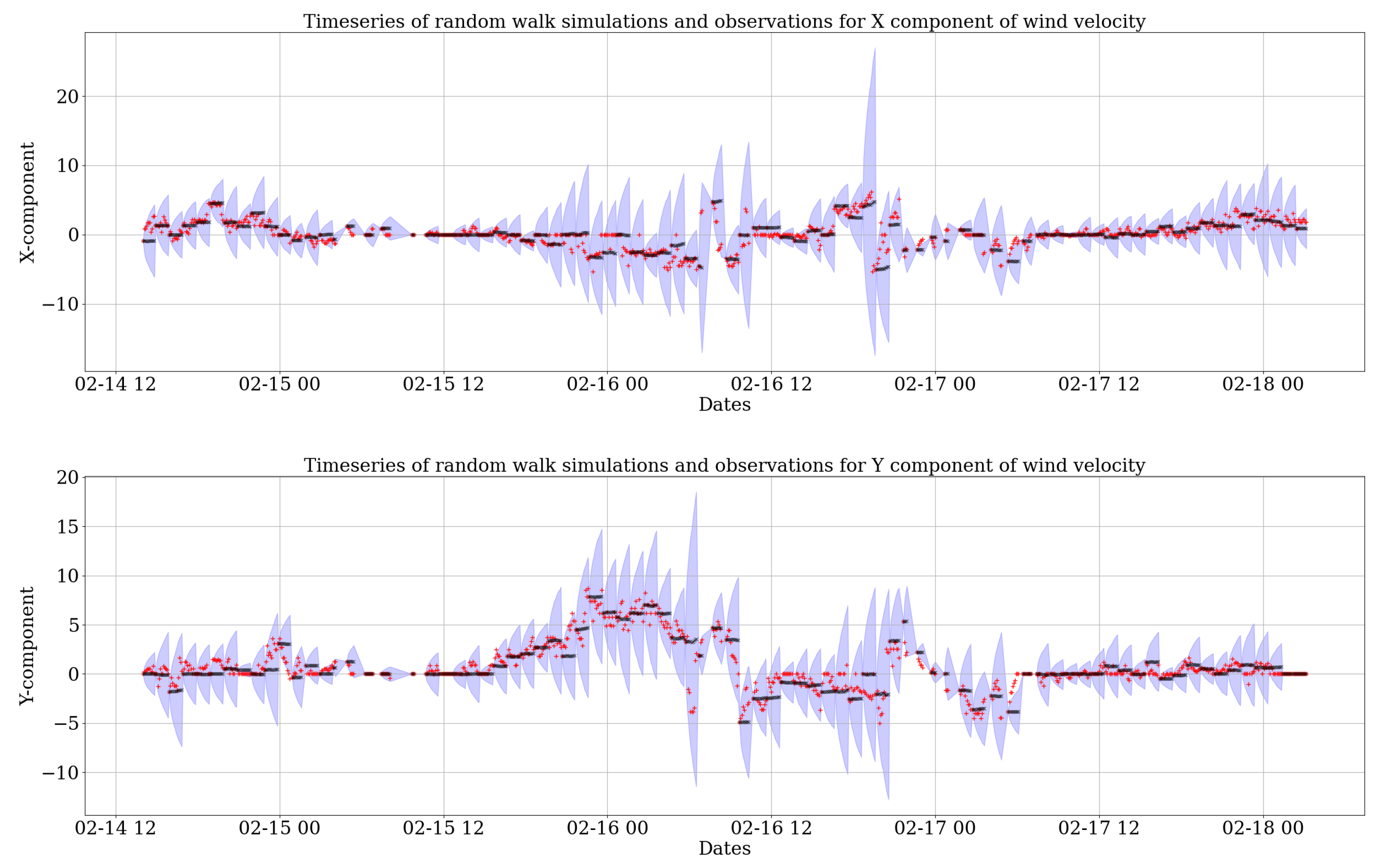
The resulting predictions for 3 days (14–18 February 2014) can be seen in two sets of time series in Figure 2 and Figure 3. For each simulation, 1000 realizations were computed. Then, the mean of all of these realizations was compared to the observations to assess how well the model fits the recorded wind data.
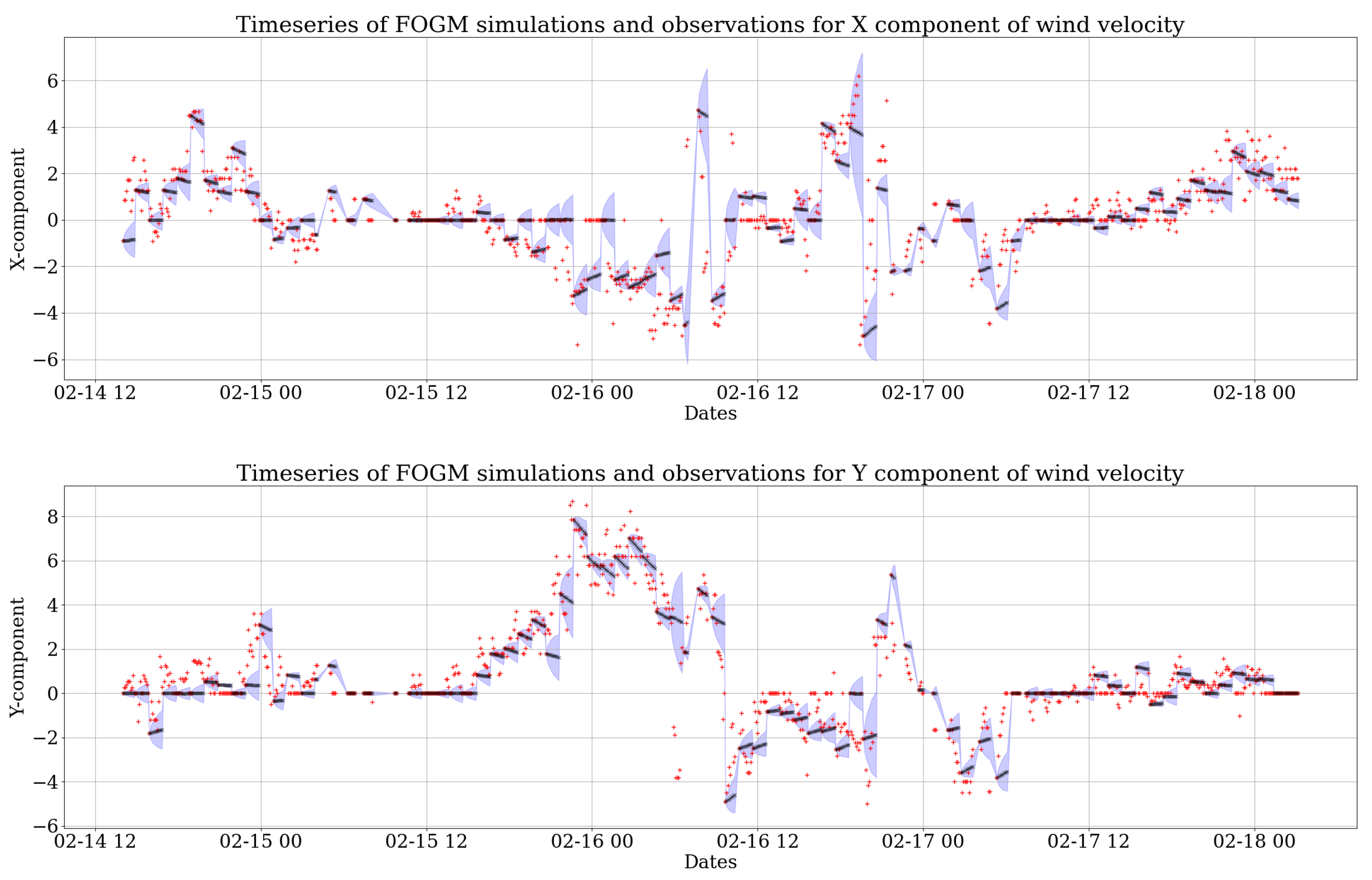
Figure 2 shows the resultant components of wind velocity predicted by the random walk process. The prediction bands of the 1000 realizations in blue show where one expects the simulated data to lie. The black dots give the mean of the 1000 realizations at each time step. It is clear that the mean prediction (black) is very close to the red stars representing the wind velocity observations. Similarly, Figure 3 shows the predictions from the fogm model. By comparing Figure 2 and Figure 3, it is clear that the variability created by the random walk model is larger than the fogm process. This is due to the fact that fogm is a mean-reverting process, which is always naturally bounded and maintains the data around a value, while the prediction band of the random walk simulation tends to cover a higher scatter. However, the mean of 1000 realizations of both stochastic processes (black dots in Figure 2 and Figure 3) behave very similarly to the observations of each wind component and also each other.
An evaluation of both the stochastic wind models was performed for the collected data from all 11 weather stations, which resulted in very similar outcomes. In general, the results show that the fogm process gives smaller uncertainties for wind modeling compared to the random walk process. The prediction bands of the fogm process are also much narrower than the bands of the random walk. This is due to the fact that the different simulations of the fogm process are much closer to each other compared to the random walk as a result of the mean-reverting characteristic of the fogm process. However, the means of both stochastic processes exhibit similar behavior and fit very well the observed wind data. This will be further assessed by validating the stochastic wind models in the next section.
3.3. Validation of Estimated Noises for Data Collected from Weather Stations
The simulations were evaluated using the root mean square error (rmse). If represents the data predicted using a stochastic process model and represents the observed data, then the rmse is calculated as
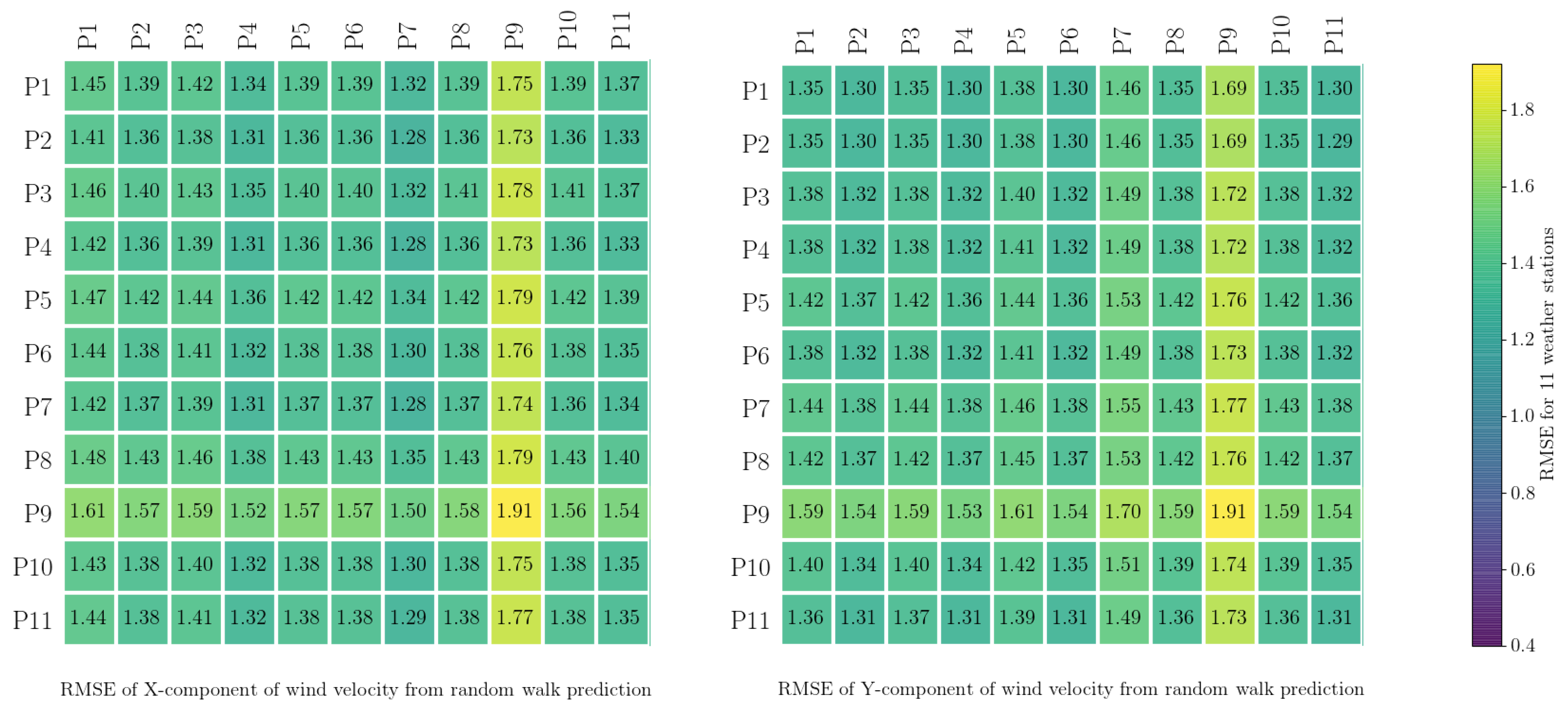
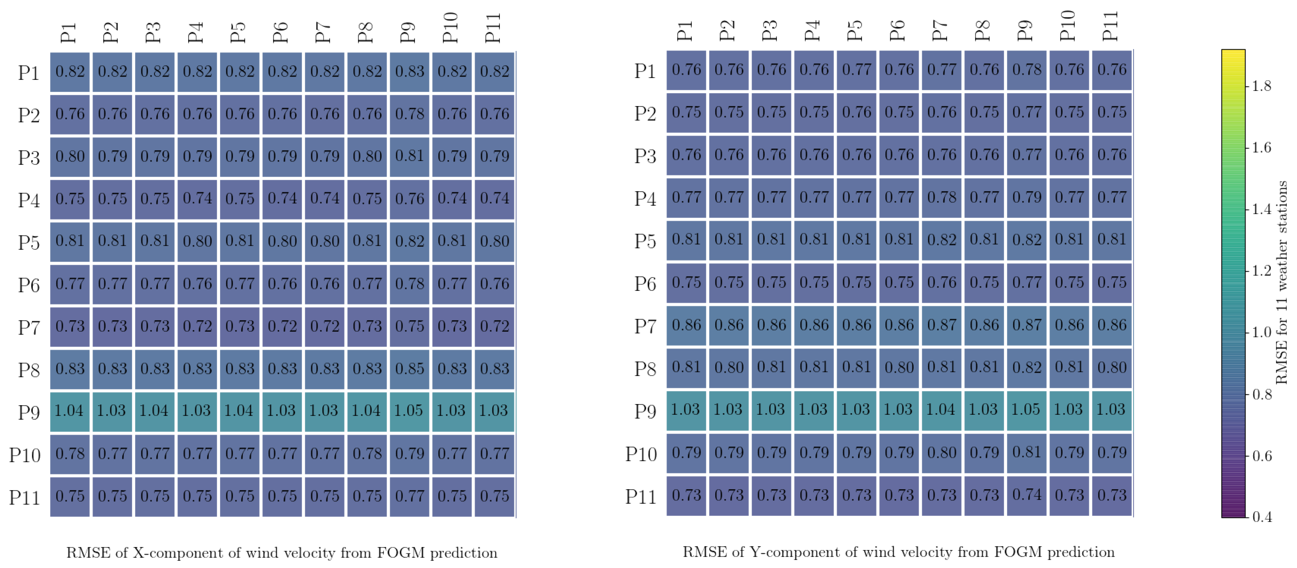
where rmse is calculated for the simulations described in the previous section using both the random walk and fogm processes for all 11 weather stations. For every hourly interval, the corresponding estimated process noise is applied to predict the wind components; then, the rmse is calculated for that hourly duration. The average of all calculated rmse for all time intervals was then calculated as the rmse of the predicted data for each weather station. Additionally, for the sake of the validation of the process noises, the calibrated process noises from each weather station were implemented to model the data for every other station, and, again, the rmse was calculated for each station to understand how valid these estimated process noises were for different spatial positions. The results are presented in Figure 4 and Figure 5. From Figure 4 and Figure 5, it can be seen that the rmse from applying the process noises estimated from a particular station to other stations is not generally much different from the rmse for that particular station. For example, the rmse of the predicted x-component at station paw1 (p1), resulting from the estimated fogm process noise for the same station, is about , whereas using the same process noise for all the other stations results in a similar range for rmse. This shows that, for this case study, the estimated process noise from the data recorded by any particular weather station is similar to all the other stations. This is as it should be, as all of the weather stations were in close proximity to each other and so were sampling very similar local wind conditions.
The calculated rmse for the random walk process (Figure 4) is, in general, slightly larger than the calculated rmse for the fogm process (Figure 5). In these figures, the results for weather station p9 stand out slightly, and the reason for this is that the duration of data collection for this station was shorter than for the others, as mentioned in Section 2.1.
The results of the stochastic wind simulations in Figure 2 and Figure 3 and the calculated rmse values in Figure 4 and Figure 5 show that the fogm model produces predictions closer to the observed data when compared to the Wiener model and considering each and every realization of the simulations. The reason is that the fogm process is a mean-reverting process, so it is naturally bounded and more confined, whereas the Wiener process tends to fluctuate more widely because of its unrestrained variance.
3.4. Comparison of the Stochastic Simulation Distributions
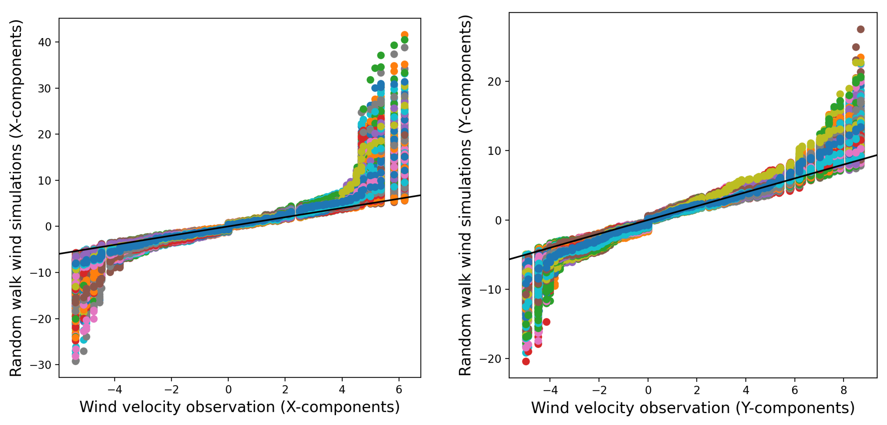
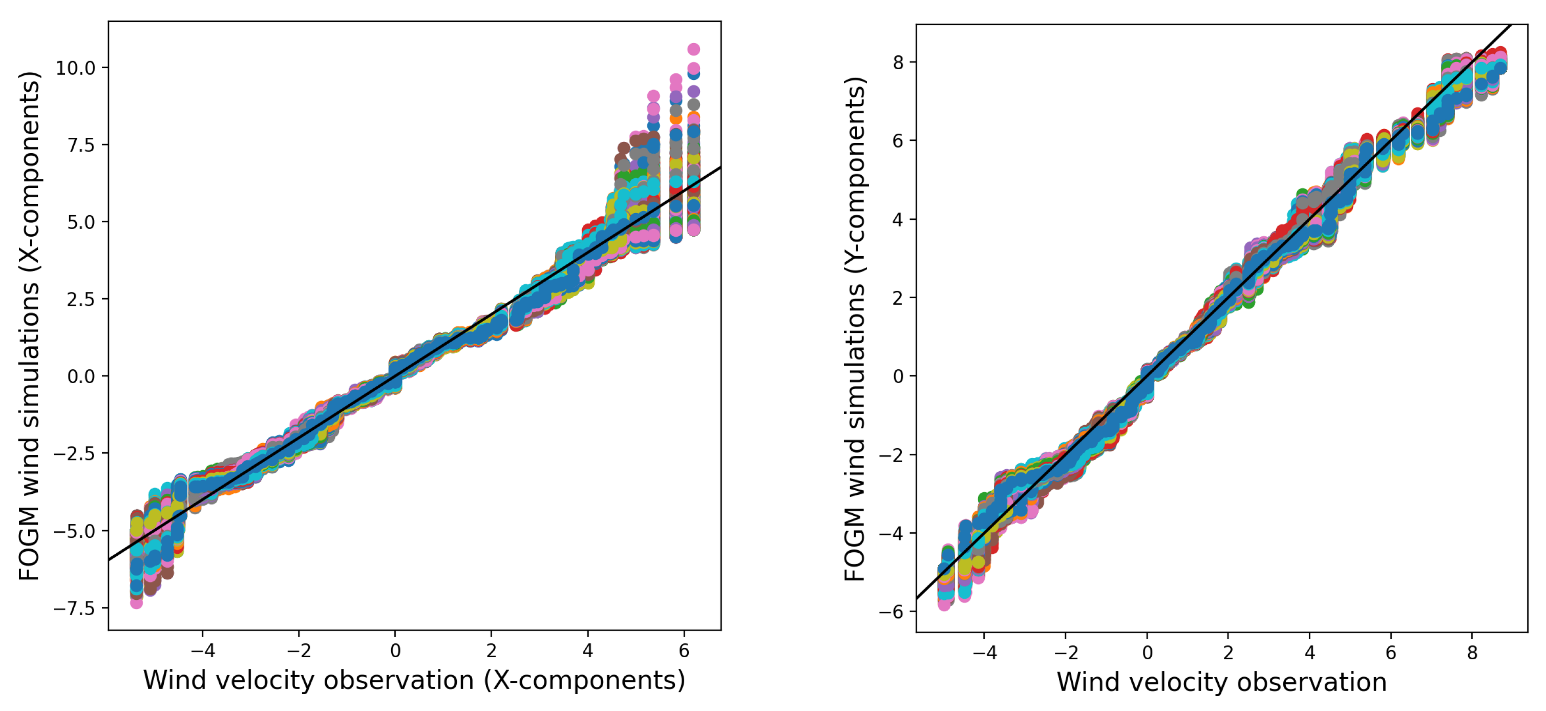
In order to assess the similarity between the distributions of the stochastic wind simulations and the wind observations, Quantile-Quantile (q-q) plots are used. Figure 6 and Figure 7 use q-q plots to compare 1000 simulated wind data points from two models from real wind observations. The models include a random walk process for the wind velocity components (x and y) and a fogm process. The comparison helps assess how closely the models’ distributions match the observed data. The simulations are based on estimated process noises, and all data are taken from paw1 over a 3-day period (14–18 February 2014).
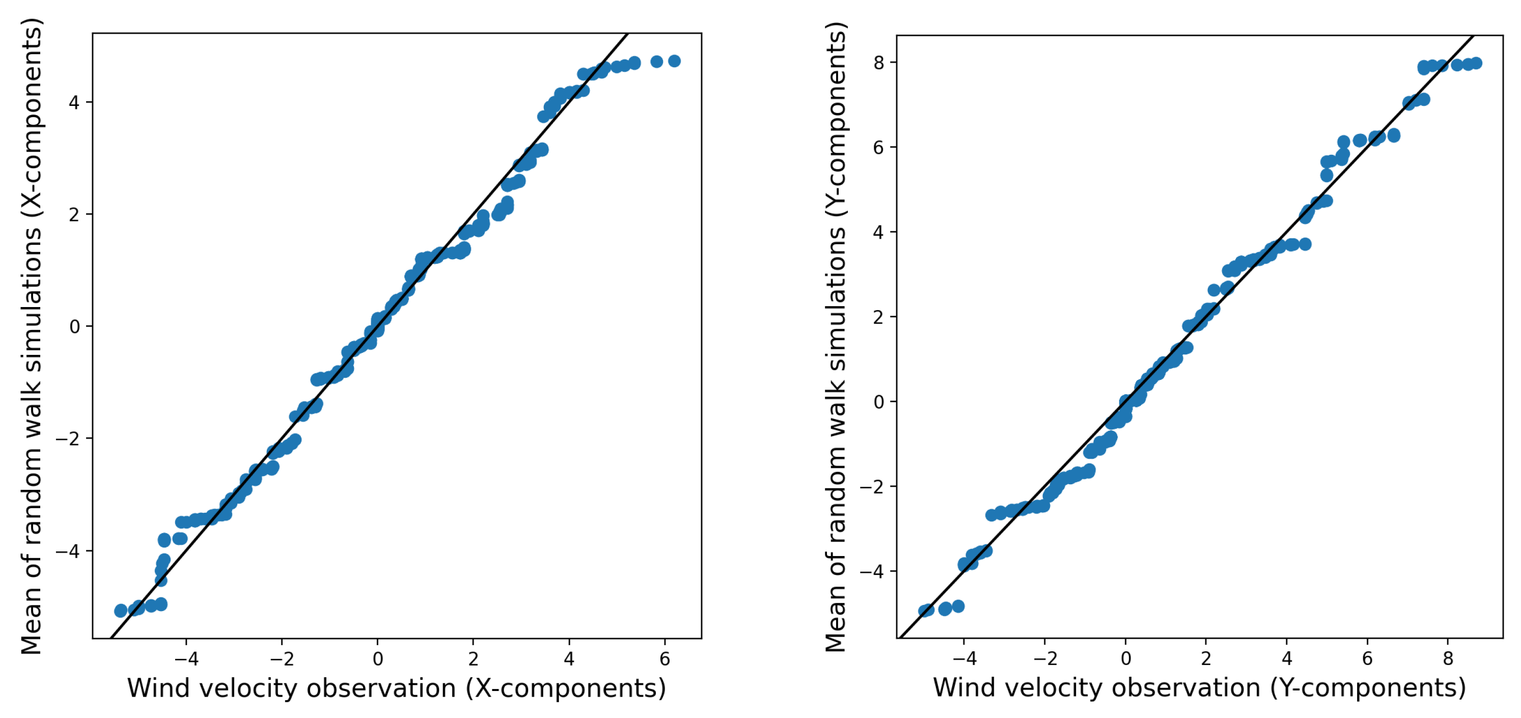
Figure 6 reveals that the random walk simulations exhibit fat tails, indicating greater variability and possible disparities in the extreme values when compared to the distribution seen in the wind observations. However, in Figure 8, which depicts the average of 1000 realizations of the random walk simulations, these fat tails are less evident. The mean of the simulations seems to closely correspond to the distribution of the observed wind data. This suggests that the random walk model accurately captures the central tendencies and general patterns of wind behavior.
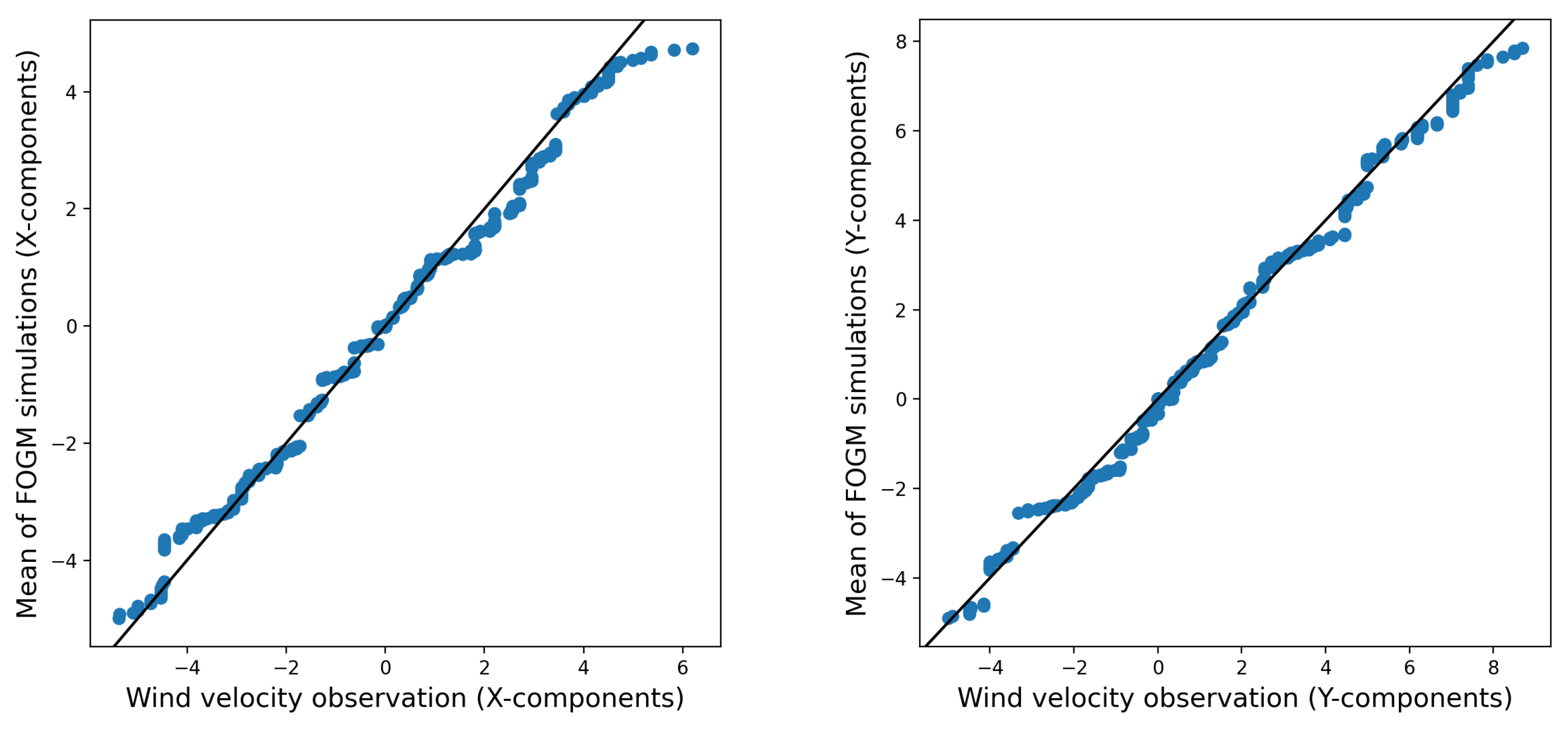
Conversely, the average of 1000 realizations from the fogm process behaves in a very similar manner to the average of 1000 realizations from the random walk simulation. Additionally, both averages closely align with the wind observations (as shown in Figure 8 and Figure 9). This indicates that although the fogm process generally produces less variation among different simulations and generates values that are nearer to the observed data compared to the random walk simulation (see Figure 7), the means of the realizations for both stochastic processes are similar and closely resemble the observed data.
It is important to note, however, that obtaining a sufficient number of realizations to accurately capture the average outcomes can be computationally demanding and time-intensive. This aspect provides the fogm process with an advantage over the random walk process.
4. Fire Simulation
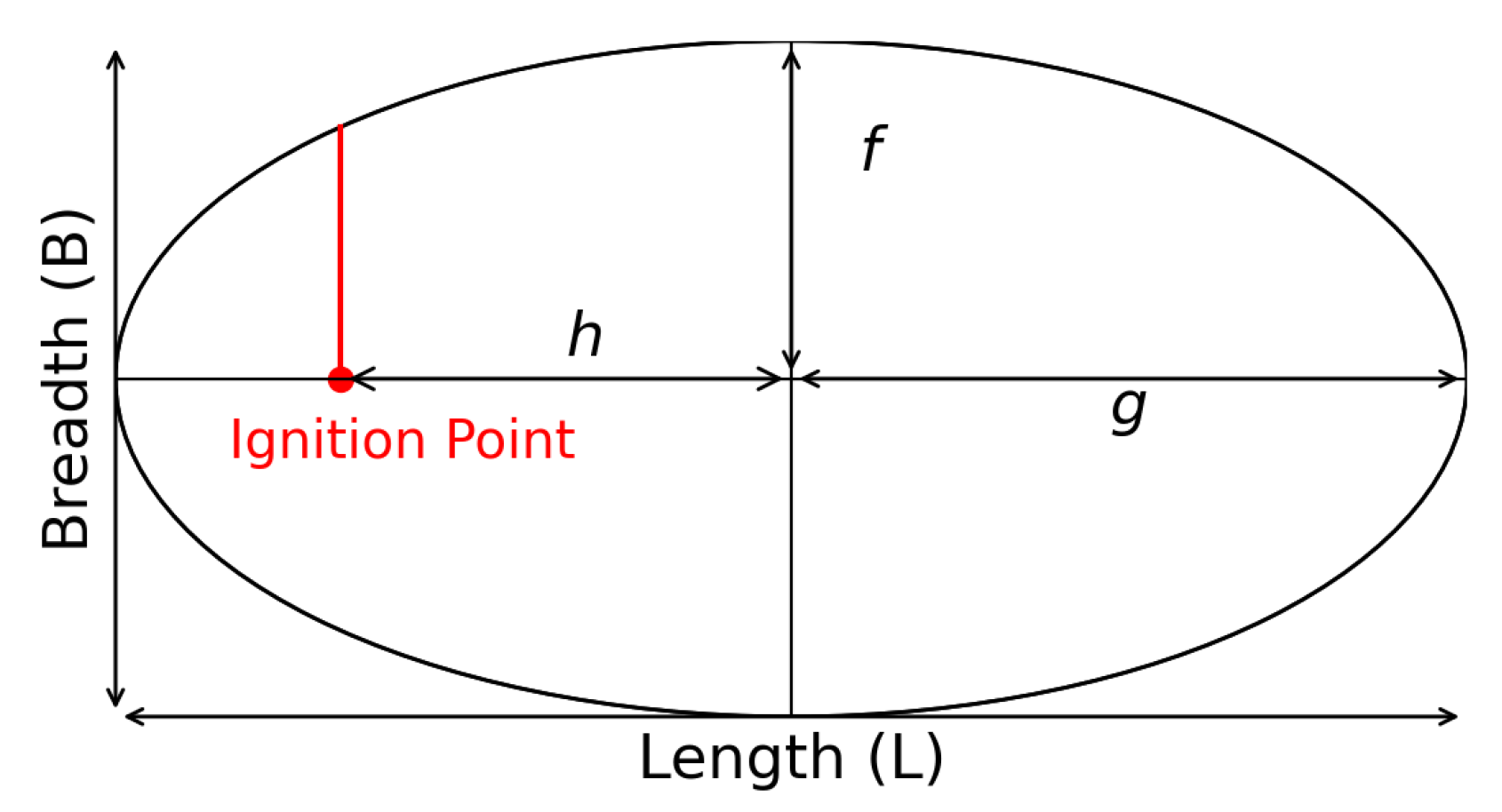
Normally, in rate-of-fire spread simulations, the fire perimeter in two-dimensional space can be modeled based on an elliptic Huygen principle [14]. We employ such a model here, with shape parameters f, g, and h, as depicted in Figure 10.
The model describes a fire moving with a speed determined by the wind, which is related to the length-to-breadth ratio, , of the elliptic stencil [45]. The spread of the elliptical fire in this model can be described as a normal flow, with the speed given by Robert et al. [42]:
where is the unit normal vector to the fire perimeter, and is the wind direction vector, and
with the head-to-back fire rate-of-spread ratio, , given by
In order to implement the calibrated stochastic wind models in a fire spread model, the spark fire spread simulator is used. In this framework, the elliptical fire model can be applied, as well as other deterministic models where the growth of the fire front can be calculated by tracking the distance between the points on the front and the points in a specific domain using the level set method [46]. The level set method uses the signed distance as the level set function of a closed curve, which is the fire perimeter; if a point is inside the curve, the signed distance function is negative (); if it is outside the curve, the function is positive (); otherwise, the function is zero, which means that the point is located on the boundary of the curve (). The zero-level set at each time step represents the new fire front at that time step. In other words, the spark framework is able to track the outward evolution of the fire front, with the speed, s, at each point on the fire boundary given using the following equation for the level set function:
Wind is an important factor in the spark framework. The fire simulator tracks the direction of fire growth with respect to the wind vector, which can potentially change the direction and the wind speed of the fire, which affects the dimensional parameters of the elliptical stencil via the length-to-breath ratio (stronger winds correspond to a larger length-to-breadth ratio).
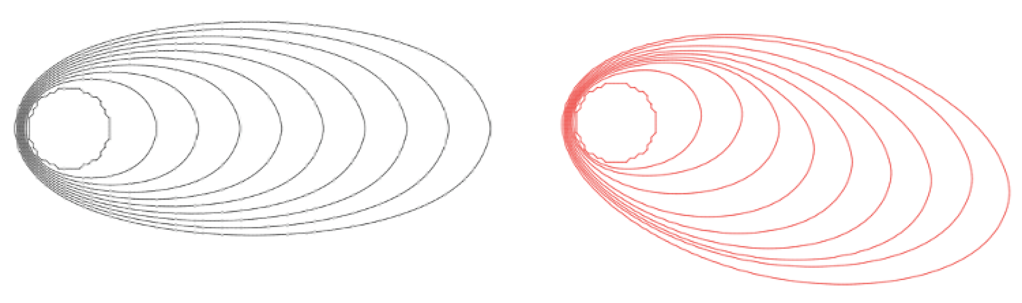
In order to integrate the newly introduced stochastic wind model into the spark solver and adjust the wind components stochastically, the stochastic wind models have been integrated into the level set solver. Subsequently, the spark solver gains access to and utilizes these models within the advection model. This facilitates the dynamic and stochastic modification of the advect-x and advect-y components, ensuring that the variability of the wind is adequately accounted for during the simulation. The script demonstrates how to pass the random walk wind model to the solver. Figure 11 displays a comparison between the deterministic fire spread model without the implemented stochastic wind models and the fire model with the implemented FOGM wind model, which updates both wind vector components at each time step. The natural variability of wind components throughout the fire simulation is clearly noticeable.
config = {
‘‘resolution’’: 1.0,
‘‘advectionScript’’: ’’’
advect_x = sqrt(dt)∗0.03∗randomNormal(0,1);
advect_y = sqrt(dt)∗0.03∗randomNormal(0,1);’’’
... #buildScript and initialisations if it is needed
}
solver = LevelSet()
solver.init(json.dumps(config), v, inputVariables = variables)
...
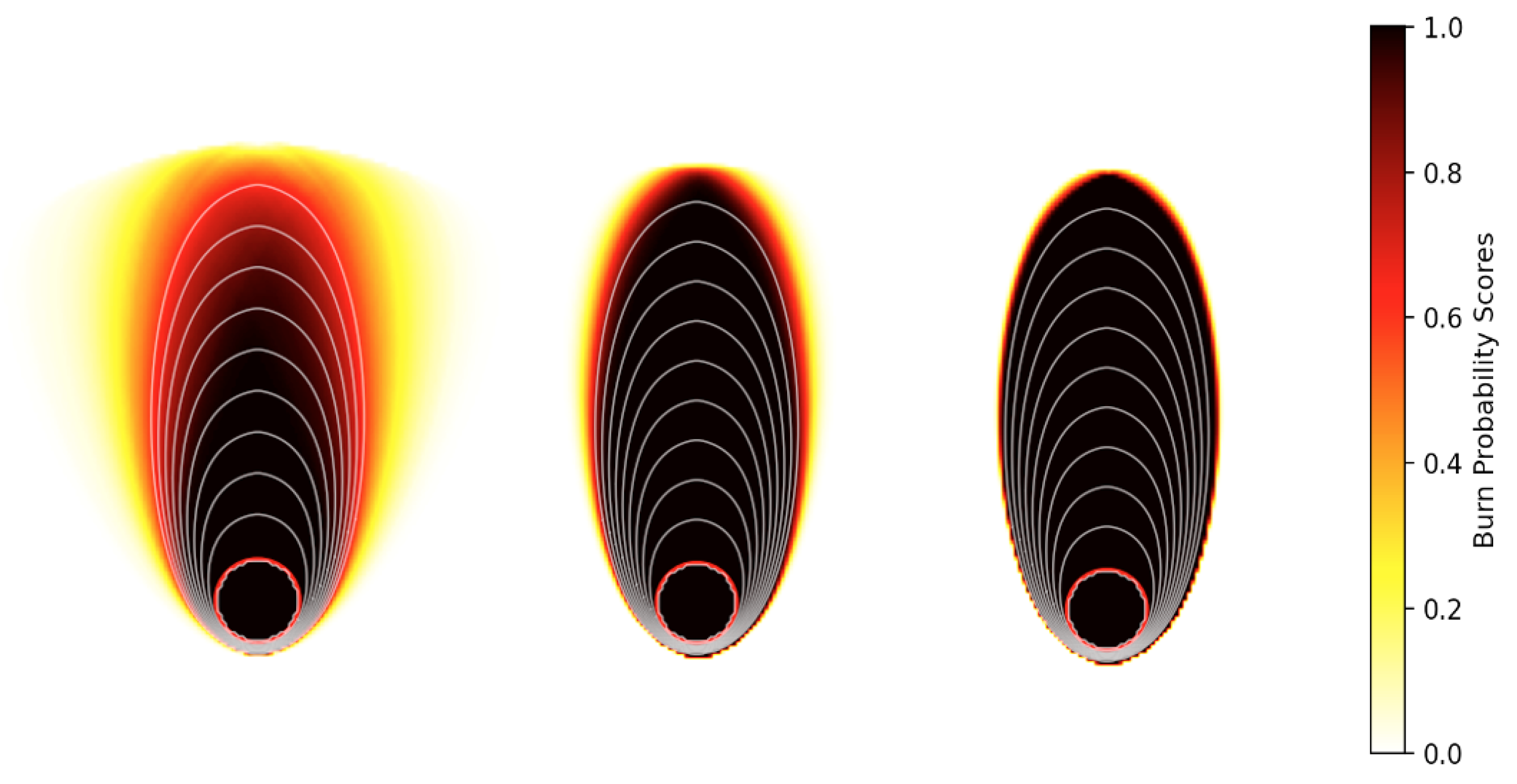
The stochastic nature of the wind models presented in this study gives variability in the results of the fire spread simulations, so every realization of the same simulation represents a different fire front. In order to visualize the different possibilities of stochastic wind models, each of the simulations was run 1000 times. The fire spread simulations are executed using various integrated wind models, including ensemble-deterministic, the fogm process, and the random walk process; the estimated statistics from the paw stations are utilized, as shown in Table 3. Besides applying probabilistic approaches to capture the intrinsic uncertainty in wildfire spread, probability maps [22] can be useful aids in visualizing the possible scenarios of burnt and unburnt regions. The fire spread simulations in spark, coupled with the different stochastic wind models, are visualized by burn probability maps displayed in Figure 12. Darker colors show the locations that have higher burn probability scores in comparison with the lighter colors, which are less likely to burn.
Figure 12 shows three different fire scenarios simulated by different probabilistic wind models, including a deterministic ensemble (with distributed inputs generated by a normal distribution, with estimated mean and variance from the observed data), the random walk process, and the fogm process. In general, the stochastic approaches present a smaller range of uncertainty related to the wind vector; the regions with darker colors and the higher burn probabilities are larger for boththe random walk and fogm processes when compared to the ensemble simulation on the left side of Figure 12. Additionally, the implemented fogm process in the fire simulation shows less uncertainty compared to the random walk simulation, as would be expected from previous observations.
5. Discussion
Incorporating time series derived from stochastic wind velocity simulations has the potential to extend the capability of bushfire modeling to capture the intrinsic stochastic variation of fire propagation. Both stochastic wind models considered here supported this capability, even though they exhibited slightly different results. The resulting fire simulations provide more useful and well-informed predictions compared to the deterministic ensemble simulations in terms of risk assessment. The time series of the ensemble of the random walk model follows the observed variability in the wind components over time with a broader band for the prediction compared to the time series of the ensemble fogm prediction. Although the distribution of every realization might not fit the observed values very well in Figure 6 and Figure 7, the average of the different realizations gives predictions that are very close to the wind observations in Figure 8 and Figure 9. The fat-tailed q-q plots for the random walk simulations confirm this observation. The random walk model is able to introduce uncertainty into the wind factor for fire spread simulation, with a narrower uncertainty band for the probability of burning compared to the deterministic ensemble model.
On the other hand, the individual realizations of the ensemble fogm model produce very similar wind predictions to the wind observations, which can be observed in the time series of the simulations, as well as the resultant thin tail q-q plots. Even though the individual realizations of the random walk model sometimes produce simulations less similar to the observed data than the fogm model, the average of all the ensemble members from both models shows similar outcomes that represent the observed data very well (shown in Figure 8 and Figure 9). Implementing the fogm wind model in spark exhibits an even narrower band of uncertainty in the burned probability map compared to the fire spread models for both the implemented random walk wind prediction and the deterministic ensemble.
The information conveyed from different burn probability maps has the potential to better inform the decision-making of fire management personnel, as they provide an estimate of the relative likelihood of different regions being burnt in a particular fire event. Implementing the deterministic and stochastic wind models with different associated levels of uncertainty provides insights into the different levels of risk that apply in various forecast scenarios. These insights can then assist expert fire behavior analysts in making predictions about likely fire progression and the associated decisions related to resource allocation or public evacuation. Future work will examine how to best capture the intrinsic variability of real wildfires, as the over-estimation of fire propagation can result in the needless allocation of resources or public evacuations, whereas the under-estimation of fire propagation can have far more dire consequences. Overall, it is important to employ models that more faithfully and accurately account for the processes that underpin the intrinsic variability of fire spreading and better capture the many uncertainties that make wildfire spread prediction such a challenging task.
The data used in this study were collected from a particular location characterized as flat grassland, which may not be representative of more general environments where fires may burn. The uniqueness of the data originating from multiple stations in close proximity to the same location is exceptionally rare. As such, the estimated process noises may not be applicable for other locations that do not match the particular wind characteristics considered here. Applying stochastic wind models as part of bushfire simulations in different locations—especially those in complex forested terrain—would require similar but separate analyses to determine the process noises and the validity of the stochastic wind models. This would be an essential requirement in extending the model across different geographical conditions. Nevertheless, the process noise levels estimated in this study can provide a good indication for realistic noise levels to be used when implementing stochastic processes to simulate wind data.
6. Conclusions
This study has demonstrated the use of stochastic wind modeling as a supplement to traditional fire propagation modeling, highlighting the importance of accounting for the intrinsic uncertainty of environmental processes in improving the accuracy and reliability of fire propagation models.
We compared the performance of two stochastic models—random walk and fogm processes—in predicting the temporal variation of wind vectors using a dataset of hourly wind observations from a meteorological station located in a wildfire-prone area in Australia. We found that the fogm model outperformed the random walk model in terms of capturing the temporal correlation of wind vectors and producing more accurate predictions of wind speed and direction. Furthermore, we used the predicted wind vectors as inputs to a wildfire spread model to investigate the sensitivity of wildfire behavior to the accuracy of the wind inputs. We found that even small changes and variability in the wind direction and speed can lead to significant differences in the predicted wildfire behavior.
In conclusion, this study underscores the significance of integrating stochastic wind modeling into fire propagation models, showcasing the pivotal role of accounting for inherent environmental uncertainties. By demonstrating the impact of accurate wind inputs on wildfire predictions, our findings highlight the critical need for precise and reliable wind data to improve the overall efficacy of fire spread models and enhance wildfire management strategies. This study could be significantly expanded and enriched by incorporating various datasets from diverse situations and regions. While our current analysis is based on a single dataset of wind data only over two months, we recognize that the inclusion of longer datasets from different geographical areas and scenarios would enhance the comprehensiveness of this research. Therefore, we acknowledge the potential for future research to explore the incorporation of additional datasets.
Author Contributions
Methodology, S.M., J.S., Z.J. and I.T.; validation, S.M.; formal analysis, S.M.; data curation, S.M.; writing—original draft preparation, S.M.; writing—review and editing, J.S., Z.J., I.T. and S.W.; visualization, S.M.; supervision, J.S., Z.J. and I.T.; funding acquisition, S.M. and J.S. All authors have read and agreed to the published version of the manuscript.
Funding
This research was funded by a University of New South Wales Canberra International Student Scholarship; the funder is UNSW Canberra.
Institutional Review Board Statement
Not applicable.
Informed Consent Statement
Informed consent was obtained from all subjects involved in the study.
Data Availability Statement
Restrictions apply to the availability of this data. The data were provided by Racheal Quill and can be accessed through the authors with Racheal Quill’s permission.
Acknowledgments
I extend my acknowledgment to Rachel Quill for her role in curating the wind data that were utilized in this study. Additionally, I am grateful to James Hilton for his invaluable support in executing the SPARK simulations. Lastly, I would like to express my deep appreciation for the invaluable support provided by the UNSW Bushfire Group, which was instrumental in the successful completion of this research endeavor.
Conflicts of Interest
The authors declare no conflict of interest.
References
- Molina-Terrén, D.M.; Xanthopoulos, G.; Diakakis, M.; Ribeiro, L.; Caballero, D.; Delogu, G.M.; Viegas, D.X.; Silva, C.A.; Cardil, A. Analysis of forest fire fatalities in southern Europe: Spain, Portugal, Greece and Sardinia (Italy). Int. J. Wildland Fire 2019, 28, 85–98. [Google Scholar] [CrossRef]
- Moore, P.F. Global wildland fire management research needs. Curr. For. Rep. 2019, 5, 210–225. [Google Scholar] [CrossRef]
- Zong, X.; Tian, X.; Yao, Q.; Brown, P.M. An analysis of fatalities from forest fires in China, 1951–2018. Int. J. Wildland Fire 2022, 31, 507–517. [Google Scholar] [CrossRef]
- Abram, N.J.; Henley, B.J.; Sen Gupta, A.; Lippmann, T., Jr.; Clarke, H.; Dowdy, A.J.; Sharples, J.J.; Nolan, R.H.; Zhang, T.; Wooster, M.J. Connections of climate change and variability to large and extreme forest fires in southeast Australia. Commun. Earth Environ. 2021, 2, 2662–4435. [Google Scholar] [CrossRef]
- Canadell, J.G.; Meyer, C.P.; Cook, G.D.; Dowdy, A.; Briggs, P.R.; Knauer, J.; Pepler, A.; Haverd, V. Multi-decadal increase of forest burned area in Australia is linked to climate change. Nat. Commun. 2021, 12, 6921. [Google Scholar] [CrossRef] [PubMed]
- Dupuy, J.L.; Fargeon, H.; Martin-StPaul, N.; Pimont, F.; Ruffault, J.; Guijarro, M.; Hernando, C.; Madrigal, J.; Fernandes, P. Climate change impact on future wildfire danger and activity in southern Europe: A review. Ann. For. Sci. 2020, 77, 35. [Google Scholar] [CrossRef]
- Filkov, A.I.; Ngo, T.; Matthews, S.; Telfer, S.; Penman, T.D. Impact of Australia’s catastrophic 2019/20 bushfire season on communities and environment. Retrospective analysis and current trends. J. Saf. Sci. Resil. 2020, 1, 44–56. [Google Scholar] [CrossRef]
- Binskin, M.; Bennett, A.; Macintosh, A. Royal Commission into National Natural Disaster Arrangements: Report; Commonwealth of Australia: Canberra, Australia, 2020.
- Johnston, F.H.; Borchers-Arriagada, N.; Morgan, G.G.; Jalaludin, B.; Palmer, A.J.; Williamson, G.J.; Bowman, D.M. Unprecedented health costs of smoke-related PM2.5 from the 2019–20 Australian megafires. Nat. Sustain. 2021, 4, 42–47. [Google Scholar] [CrossRef]
- Dickman, C.; McDonald, T. Some personal reflections on the present and future of Australia’s fauna in an increasingly fire-prone continent. Ecol. Manag. Restor. 2020, 21, 86–96. [Google Scholar] [CrossRef]
- Fons, W.L. Analysis of fire spread in light forest fuels. J. Agric. Res. 1946, 72, 93. [Google Scholar]
- Sullivan, A.L. Wildland surface fire spread modelling, 1990–2007. 1: Physical and quasi-physical models. Int. J. Wildland Fire 2009, 18, 349–368. [Google Scholar] [CrossRef]
- Cruz, M.G.; Gould, J.S.; Alexander, M.E.; Sullivan, A.L.; McCaw, W.L.; Matthews, S. Empirical-based models for predicting head-fire rate of spread in Australian fuel types. Aust. For. 2015, 78, 118–158. [Google Scholar] [CrossRef]
- Anderson, D.H.; Catchpole, E.A.; De Mestre, N.J.; Parkes, T. Modelling the spread of grass fires. ANZIAM J. 1982, 2, 451–466. [Google Scholar] [CrossRef]
- Finney, M.A.; Grenfell, I.C.; McHugh, C.W.; Seli, R.C.; Trethewey, D.; Stratton, R.D.; Brittain, S. A method for ensemble wildland fire simulation. Environ. Model. Assess. 2011, 16, 153–167. [Google Scholar] [CrossRef]
- McArthur, A.G. Fire Behaviour in Eucalypt Forests; Forestry and Timber Bureau: Canberra, Australia, 1967. [Google Scholar]
- Dabrowski, J.J.; Huston, C.; Hilton, J.; Mangeon, S.; Kuhnert, P. Towards data assimilation in level-set wildfire models using Bayesian filtering. arXiv 2022, arXiv:2206.08501. [Google Scholar]
- Mallet, V.; Keyes, D.E.; Fendell, F.E. Modeling wildland fire propagation with level set methods. Comput. Math. Appl. 2009, 57, 1089–1101. [Google Scholar] [CrossRef]
- Alexander Martin, E.; Cruz Miguel, G. Limitations on the accuracy of model predictions of wildland fire behaviour: A state-of-the-knowledge overview. For. Chron. 2013, 89, 3. [Google Scholar] [CrossRef]
- Quill, R.; Sharples, J.J.; Wagenbrenner, N.S.; Sidhu, L.A.; Forthofer, J.M. Modeling wind direction distributions using a diagnostic model in the context of probabilistic fire spread prediction. Front. Mech. Eng. 2019, 5, 5. [Google Scholar] [CrossRef]
- Wang, X.J.; Thompson, J.R.J.; Braun, W.J.; Woolford, D.G. Fitting a stochastic fire spread model to data. Adv. Stat. Climatol. Meteorol. Oceanogr. 2019, 5, 57–66. [Google Scholar] [CrossRef]
- French, I.A.; Duff, T.J.; Cechet, R.P.; Tolhurst, K.G.; Kepert, J.D.; Meyer, M. FireDST: A simulation system for short-term ensemble modelling of bushfire spread and exposure. In Advances in Forst Fire Research; Imprensa da Universidade de Coimbra: Coimbra, Portugal, 2014; pp. 1147–1158. [Google Scholar]
- Twomey, B.; Sturgess, A. Simulation Analysis-Based Risk Evaluation (SABRE) Fire: Operational Stochastic Fire Spread Decision Support Capability in the Queensland Fire and Emergency Services; Australasian Fire and Emergency Service Authority Council (AFAC): Brisbane, Australia, 2016.
- Thompson, M.; Calkin, D.; Scott, J.H.; Hand, M. Uncertainty and probability in wildfire management decision support: An example from the United States. In Natural Hazard Uncertainty Assessment: Modeling and Decision Support; John Wiley & Sons, Inc.: Hoboken, NJ, USA, 2017; pp. 31–41. [Google Scholar]
- Cruz, M.G. Monte Carlo-based ensemble method for prediction of grassland fire spread. Int. J. Wildland Fire 2010, 19, 521–530. [Google Scholar] [CrossRef]
- Hilton, J.E.; Miller, C.; Sullivan, A.L.; Rucinski, C. Effects of spatial and temporal variation in environmental conditions on simulation of wildfire spread. Environ. Model. Softw. 2015, 67, 118–127. [Google Scholar] [CrossRef]
- Bivona, S.; Bonanno, G.; Burlon, R.; Gurrera, D.; Leone, C. Stochastic models for wind speed forecasting. Energy Convers. Manag. 2011, 52, 1157–1165. [Google Scholar] [CrossRef]
- Loukatou, A.; Howell, S.; Johnson, P.; Duck, P. Stochastic wind speed modelling for estimation of expected wind power output. Appl. Energy 2018, 228, 1328–1340. [Google Scholar] [CrossRef]
- Box, G.E.; Jenkins, G.M.; Reinsel, G.C.; Ljung, G.M. Time Series Analysis: Forecasting and Control; John Wiley & Sons: Hoboken, NJ, USA, 1994. [Google Scholar]
- Arenas-López, J.P.; Badaoui, M. Stochastic modelling of wind speeds based on turbulence intensity. Renew. Energy 2020, 155, 10–22. [Google Scholar] [CrossRef]
- Turkoglu, K. Statistics Based Modeling of Wind Speed and Wind Direction in Real Time Optimal Guidance Strategies via Ornstein-Uhlenbeck Stochastic Processes. In Proceedings of the Fourth Aviation, Range, and Aerospace Meteorology Special Symposium, American Meteorological Society (AMS) 94th Annual Meeting, Atlanta, GA, USA, 2–6 February 2014. [Google Scholar]
- Zárate-Miñano, R.; Anghel, M.; Milano, F. Continuous wind speed models based on stochastic differential equations. Appl. Energy 2013, 104, 42–49. [Google Scholar] [CrossRef]
- Benth, F.E.; Di Persio, L.; Lavagnini, S. Stochastic modeling of wind derivatives in energy markets. Risks 2018, 6, 56. [Google Scholar] [CrossRef]
- Zazali, H.H.; Towers, I.N.; Sharples, J.J. Incorporating environmental uncertainty in fire spread modelling. In Proceedings of the 22th International Congress on Modelling and Simulation (MODSIM 2017), Tasmania, Australia, 3–8 December 2017; pp. 1194–2000. [Google Scholar]
- Hilton, J.; Hetherton, L.; Miller, C.; Sullivan, A.; Prakash, M. The Spark Framework; CSIRO Digital Productivity Flagship: Clayton, Australia, 2015. [Google Scholar]
- Quill, R. Statistical Characterisation of Wind Fields over Complex Terrain with Applications in Bushfire Modelling. Ph.D. Thesis, UNSW Canberra, Sydney, Australia, 2017. [Google Scholar]
- Sharples, J.J.; McRae, R.H.; Weber, R.O. Wind characteristics over complex terrain with implications for bushfire risk management. Environ. Model. Softw. 2010, 25, 1099–1120. [Google Scholar] [CrossRef]
- Martell, D.L. A Markov chain model of day to day changes in the Canadian forest fire weather index. Int. J. Wildland Fire 1999, 9, 265–273. [Google Scholar] [CrossRef]
- Ji, K.H. Transient Signal Detection Using GPS Position Time Series. Ph.D. Thesis, Massachusetts Institute of Technology, Cambridge, MA, USA, 2011. [Google Scholar]
- Ross, S.M. An Elementary Introduction to Mathematical Finance; Cambridge University Press: Cambridge, UK, 2011. [Google Scholar]
- Higham, D.J. An algorithmic introduction to numerical simulation of stochastic differential equations. SIAM Rev. 2001, 43, 525–546. [Google Scholar] [CrossRef]
- Roberts, S. A line element algorithm for curve flow problems in the plane. ANZIAM J. 1993, 35, 244–261. [Google Scholar] [CrossRef]
- Brown, R.G.; Hwang, P.Y.C. Introduction to Random Signals and Applied Kalman Filtering: With MATLAB Exercises and Solutions; John Wiley & Sons: Hoboken, NJ, USA, 1997. [Google Scholar]
- Bibbona, E.; Panfilo, G.; Tavella, P. The Ornstein–Uhlenbeck process as a model of a low pass filtered white noise. Metrologia 2008, 45, S117. [Google Scholar] [CrossRef]
- Finney, M.A. FARSITE: Fire Area Simulator-Model Development and Evaluation; US Department of Agriculture, Forest Service, Rocky Mountain Research Station: Ogden, UT, USA, 1998.
- Sethian, J.A. Level Set Methods and Fast Marching Methods, 2nd ed.; Cambridge University Press: Cambridge, UK, 1999; Volume 98. [Google Scholar]
Figure 1.
Hourly variation in wind speed () and direction during three days: 14–16 February 2014. The data shown are from station paw1.
Figure 1.
Hourly variation in wind speed () and direction during three days: 14–16 February 2014. The data shown are from station paw1.

Figure 2.
Time series of wind components x (top) and y (bottom) using random walk simulation with and for weather station paw1. The observed data are depicted by red stars, the prediction band of the 1000 realizations of the simulation by blue shaded bands, and the mean of simulation realizations by black dots. A prediction band signifies that around of predicted data fall within this band, and this is calculated approximately as , where represents the mean value of predicted wind every hour, and stands for the standard deviation of predicted values across hourly blocks.

Figure 3.
Time series of wind components x (top) and y (bottom) using fogm simulation with and for weather station paw1. The observed data are depicted by red stars, the prediction band of the 1000 realizations of simulation by blue shaded bands, and the mean of simulation realizations by black dots. Note the scale is different from Figure 2.

Figure 4.
rmse validation for 11 weather stations. The random walk process noises were estimated using the stations listed in the matrix rows, and these were implemented in the simulations for stations listed in the matrix columns.
Figure 4.
rmse validation for 11 weather stations. The random walk process noises were estimated using the stations listed in the matrix rows, and these were implemented in the simulations for stations listed in the matrix columns.

Figure 5.
rmse validation for 11 weather stations. The fogm process noises were estimated using the stations listed in the matrix rows, and these were implemented in the simulations for the stations listed in the matrix columns.
Figure 5.
rmse validation for 11 weather stations. The fogm process noises were estimated using the stations listed in the matrix rows, and these were implemented in the simulations for the stations listed in the matrix columns.

Figure 6.
q-q plots of the observed data and 1000 realizations of the simulated data: random walk process and observation. Different colors represent the randomly generated samples from each realization of the simulation.
Figure 6.
q-q plots of the observed data and 1000 realizations of the simulated data: random walk process and observation. Different colors represent the randomly generated samples from each realization of the simulation.

Figure 7.
q-q plots of the observed data and 1000 realizations of the simulated data; fogm the process and observation (scales for the fogm processes are different to make visible the smaller uncertainties compared to the random walk process). Different colors represent the randomly generated samples from each realization of the simulation.

Figure 8.
q-q plots of the observed data and the mean of 1000 realizations of the simulated data (dots in blue color): random walk and observation.
Figure 8.
q-q plots of the observed data and the mean of 1000 realizations of the simulated data (dots in blue color): random walk and observation.

Figure 9.
q-q plots of the observed data and the mean of 1000 realizations of the simulated data (dots in blue color): fogm process and observation.
Figure 9.
q-q plots of the observed data and the mean of 1000 realizations of the simulated data (dots in blue color): fogm process and observation.

Figure 10.
Dimensions of elliptical fire spread model.

Figure 11.
On the left: a deterministic fire spread model with a contour interval of 10 units of time and constant wind along the x-axis. On the right: a single realisation of the fire spread model with stochasticity implemented in Spark.
Figure 11.
On the left: a deterministic fire spread model with a contour interval of 10 units of time and constant wind along the x-axis. On the right: a single realisation of the fire spread model with stochasticity implemented in Spark.

Figure 12.
Burn probability maps of fire simulations in spark. Left: deterministic ensemble method, with 1000 realizations (the wind components are normally distributed, and the mean and standard deviations are given in Table 3). Middle: stochastic wind model using the random walk process model with calibrated process noises, , for the wind vector components. Right: stochastic wind model using the fogm process model with calibrated process noises, , for the wind vector components. Each simulation represents the propagation of a red circle with an ignition point at (1, 1) over 100 units of time, with a contour interval of 10 units of time.


Table 1.
Estimated process noises, and , for random walk and fogm processes.
| Stations | paw1 | paw2 | paw3 | paw4 | paw5 | paw6 | paw7 | paw8 | paw9 | paw10 | paw11 | |
|---|---|---|---|---|---|---|---|---|---|---|---|---|
| Process | ||||||||||||
| Random walk Process | 0.033 | 0.031 | 0.032 | 0.029 | 0.031 | 0.031 | 0.028 | 0.031 | 0.044 | 0.031 | 0.030 | |
| fogm Process | 0.071 | 0.067 | 0.069 | 0.063 | 0.068 | 0.065 | 0.061 | 0.071 | 0.093 | 0.067 | 0.065 | |
Table 2.
Estimated process noises, and , for random walk and fogm processes.
| Stations | paw1 | paw2 | paw3 | paw4 | paw5 | paw6 | paw7 | paw8 | paw9 | paw10 | paw11 | |
|---|---|---|---|---|---|---|---|---|---|---|---|---|
| Process | ||||||||||||
| Random walk Process | 0.031 | 0.029 | 0.031 | 0.029 | 0.032 | 0.029 | 0.035 | 0.031 | 0.043 | 0.031 | 0.029 | |
| fogm Process | 0.065 | 0.064 | 0.065 | 0.066 | 0.069 | 0.064 | 0.076 | 0.066 | 0.088 | 0.066 | 0.063 | |
Table 3.
The estimated statistics, including the mean and standard deviation for the wind data and the average noises for both processes across all the different paw weather stations.
Table 3.
The estimated statistics, including the mean and standard deviation for the wind data and the average noises for both processes across all the different paw weather stations.
| “paw”s Statistics | ||
|---|---|---|
| Mean ms | ≈0.5 | ≈0.2 |
| Standard deviation ms | ≈2 | ≈2 |
| “fogm” process noise ms | ≈ | ≈ |
| “Random walk” process noise m(s) | ≈ | ≈ |
Disclaimer/Publisher’s Note: The statements, opinions and data contained in all publications are solely those of the individual author(s) and contributor(s) and not of MDPI and/or the editor(s). MDPI and/or the editor(s) disclaim responsibility for any injury to people or property resulting from any ideas, methods, instructions or products referred to in the content. |
© 2023 by the authors. Licensee MDPI, Basel, Switzerland. This article is an open access article distributed under the terms and conditions of the Creative Commons Attribution (CC BY) license (https://creativecommons.org/licenses/by/4.0/).
Share and Cite
MDPI and ACS Style
Masoudian, S.; Sharples, J.; Jovanoski, Z.; Towers, I.; Watt, S. Incorporating Stochastic Wind Vectors in Wildfire Spread Prediction. Atmosphere 2023, 14, 1609. https://doi.org/10.3390/atmos14111609
AMA Style
Masoudian S, Sharples J, Jovanoski Z, Towers I, Watt S. Incorporating Stochastic Wind Vectors in Wildfire Spread Prediction. Atmosphere. 2023; 14(11):1609. https://doi.org/10.3390/atmos14111609
Chicago/Turabian StyleMasoudian, Sahar, Jason Sharples, Zlatko Jovanoski, Isaac Towers, and Simon Watt. 2023. "Incorporating Stochastic Wind Vectors in Wildfire Spread Prediction" Atmosphere 14, no. 11: 1609. https://doi.org/10.3390/atmos14111609
Note that from the first issue of 2016, this journal uses article numbers instead of page numbers. See further details here.