
Global Atmospheric δ13CH4 and CH4 Trends for 2000–2020 from the Atmospheric Transport Model TM5 Using CH4 from Carbon Tracker Europe–CH4 Inversions
 , , , , , , , , , , and
Abstract
:1. Introduction
2. Materials and Methods
2.1. CarbonTracker-Europe-CH
2.1.1. TM5
2.2. CH and CH Fluxes
2.3. Atmospheric Observations
2.3.1. CH Observations for Constraining CH Fluxes
2.3.2. CH Observations for Evaluation
2.4. Isotopic Signatures
2.5. Model Setup
2.5.1. Inversion Model—CH Only
2.5.2. TM5 Forward Model with CH
3. Results
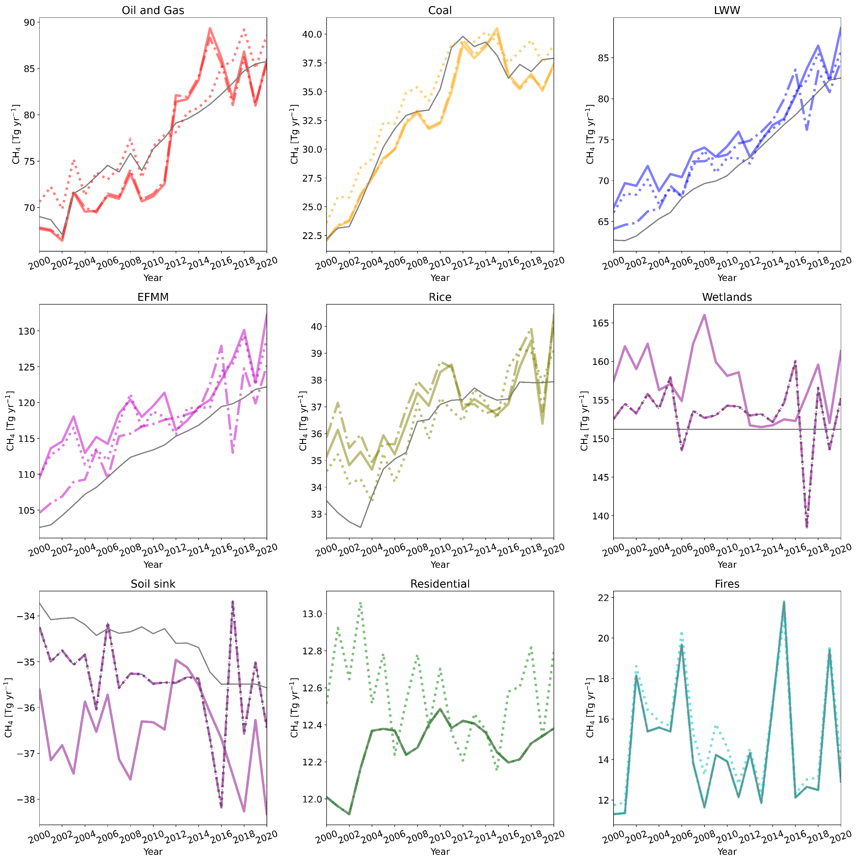
3.1. Estimated CH Fluxes
3.1.1. Estimated Emission Budgets
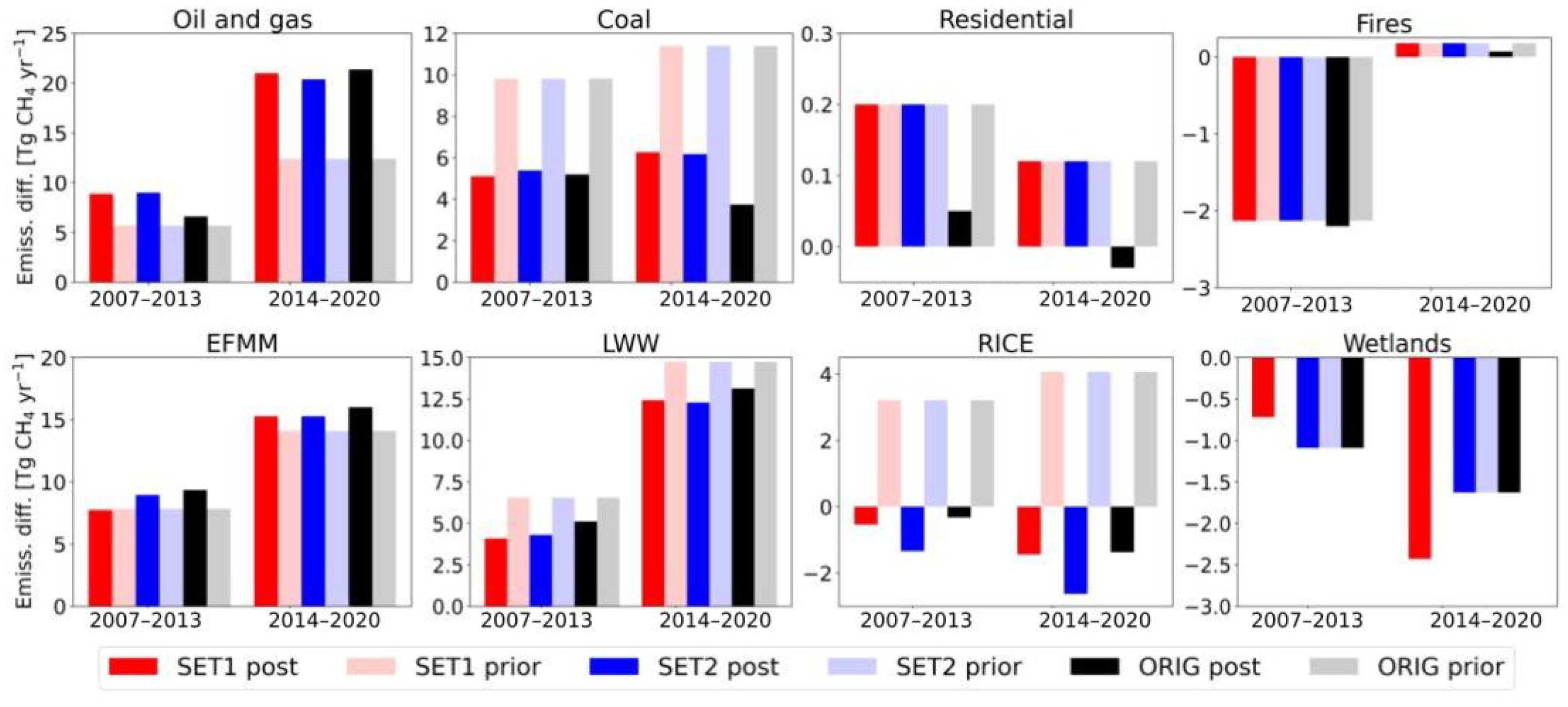
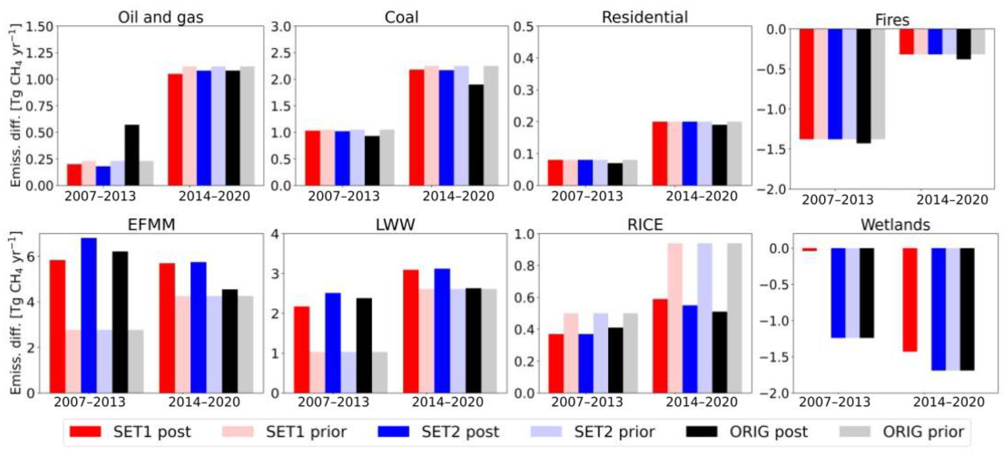
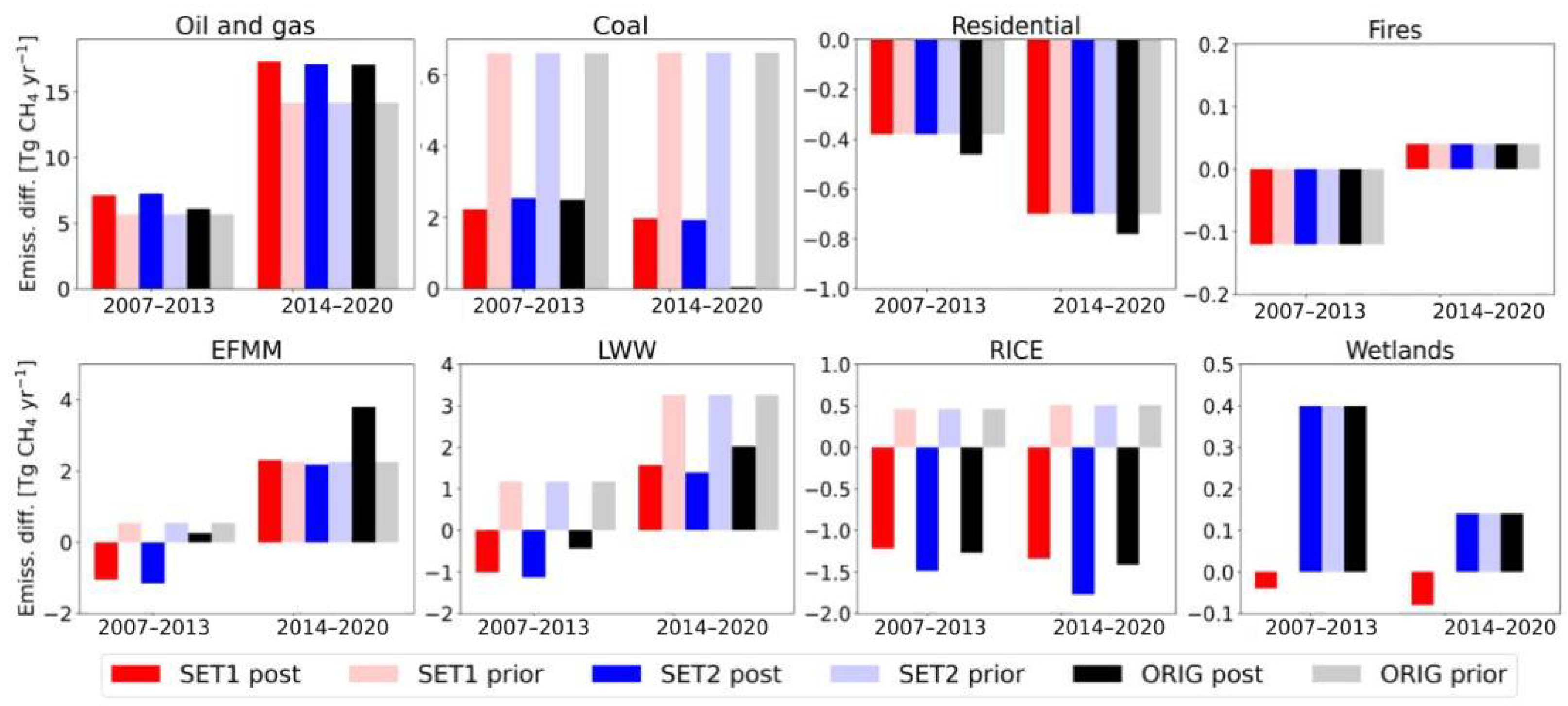
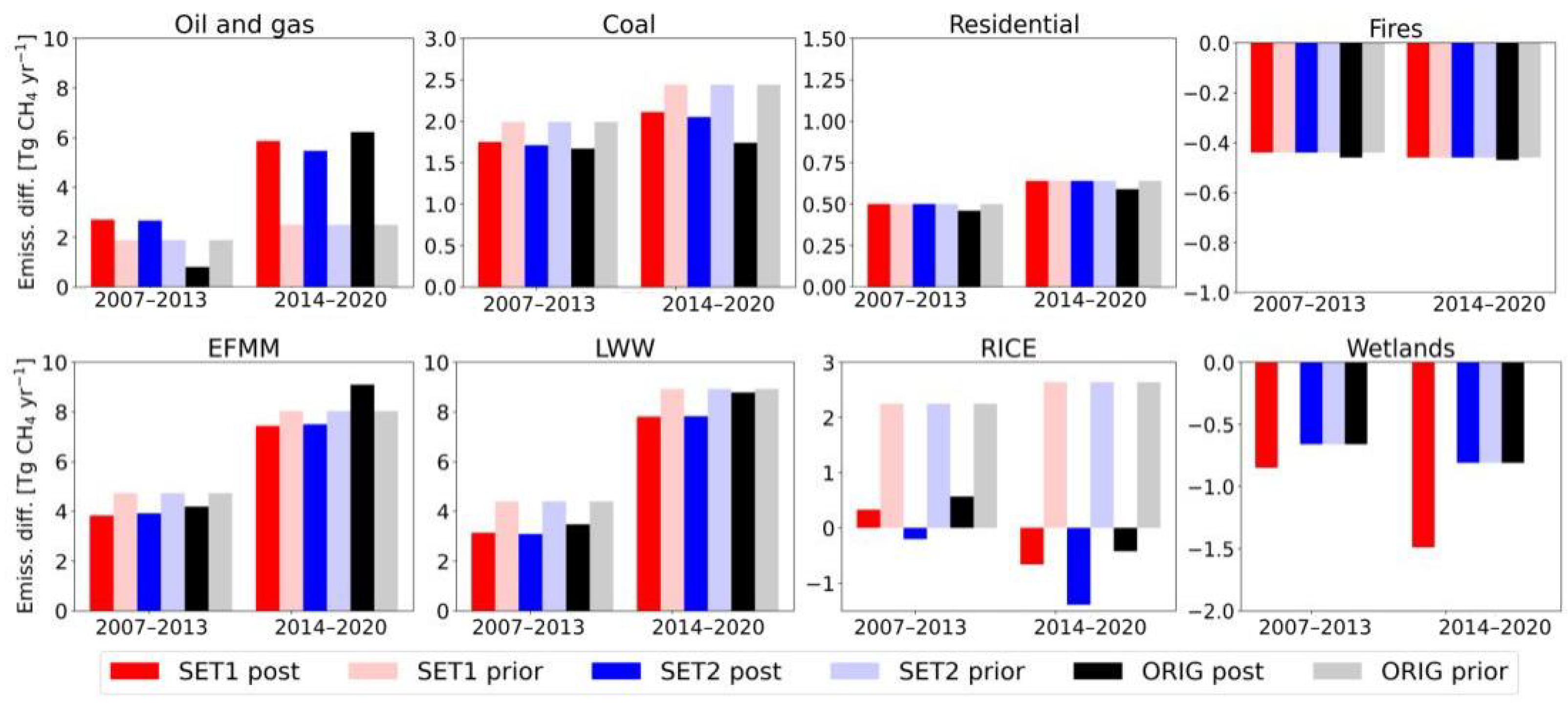
3.1.2. Emission Changes during 2000–2006, 2007–2013, and 2014–2020
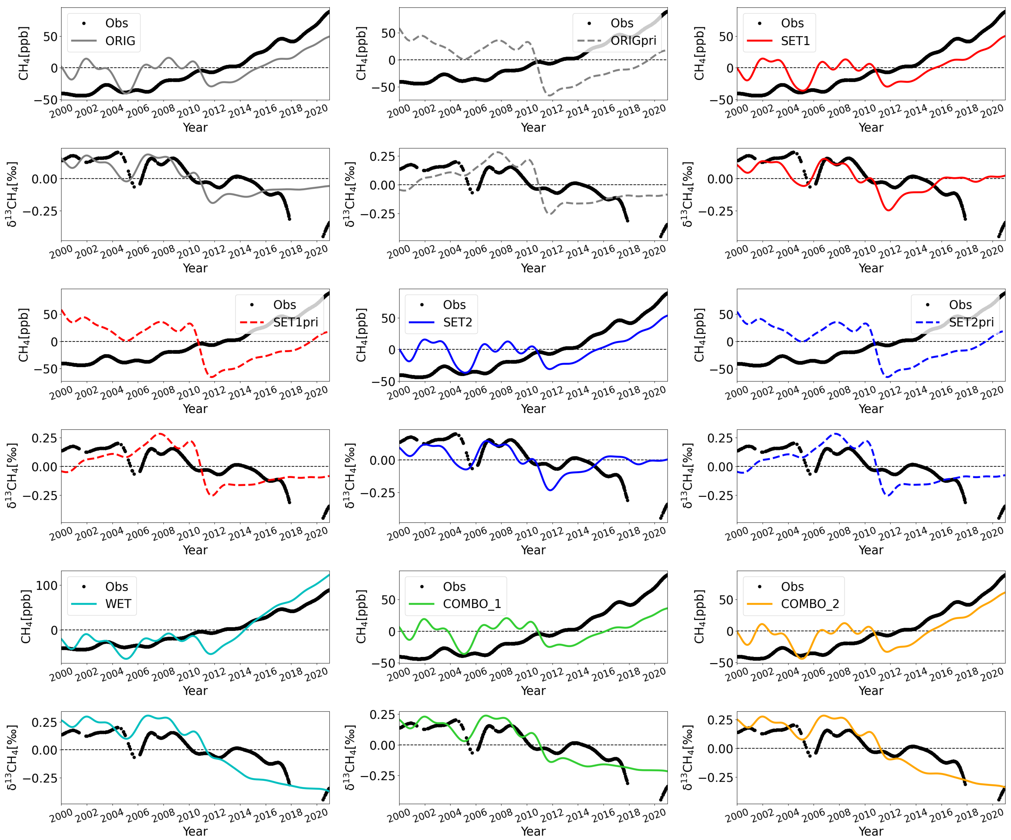
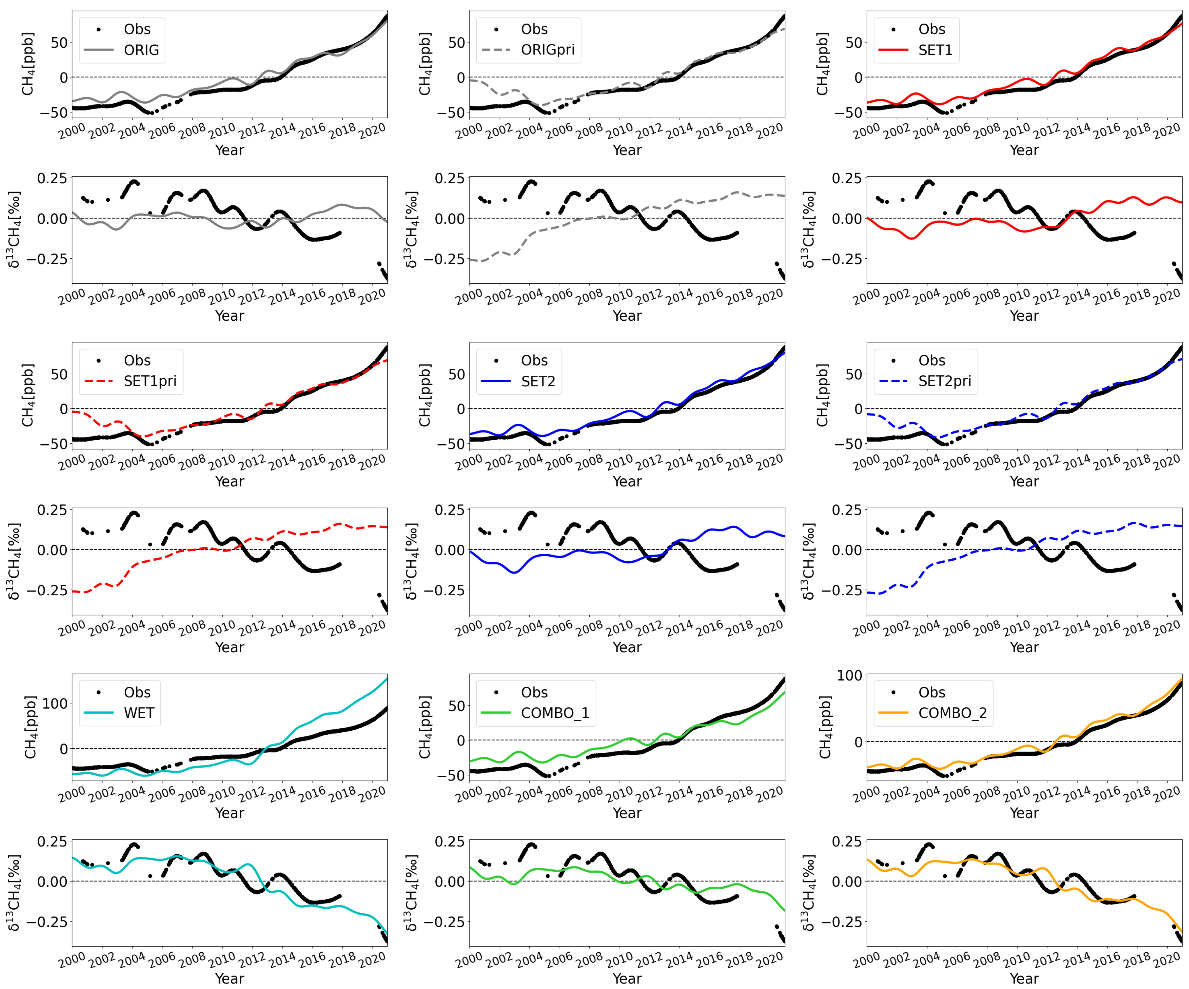
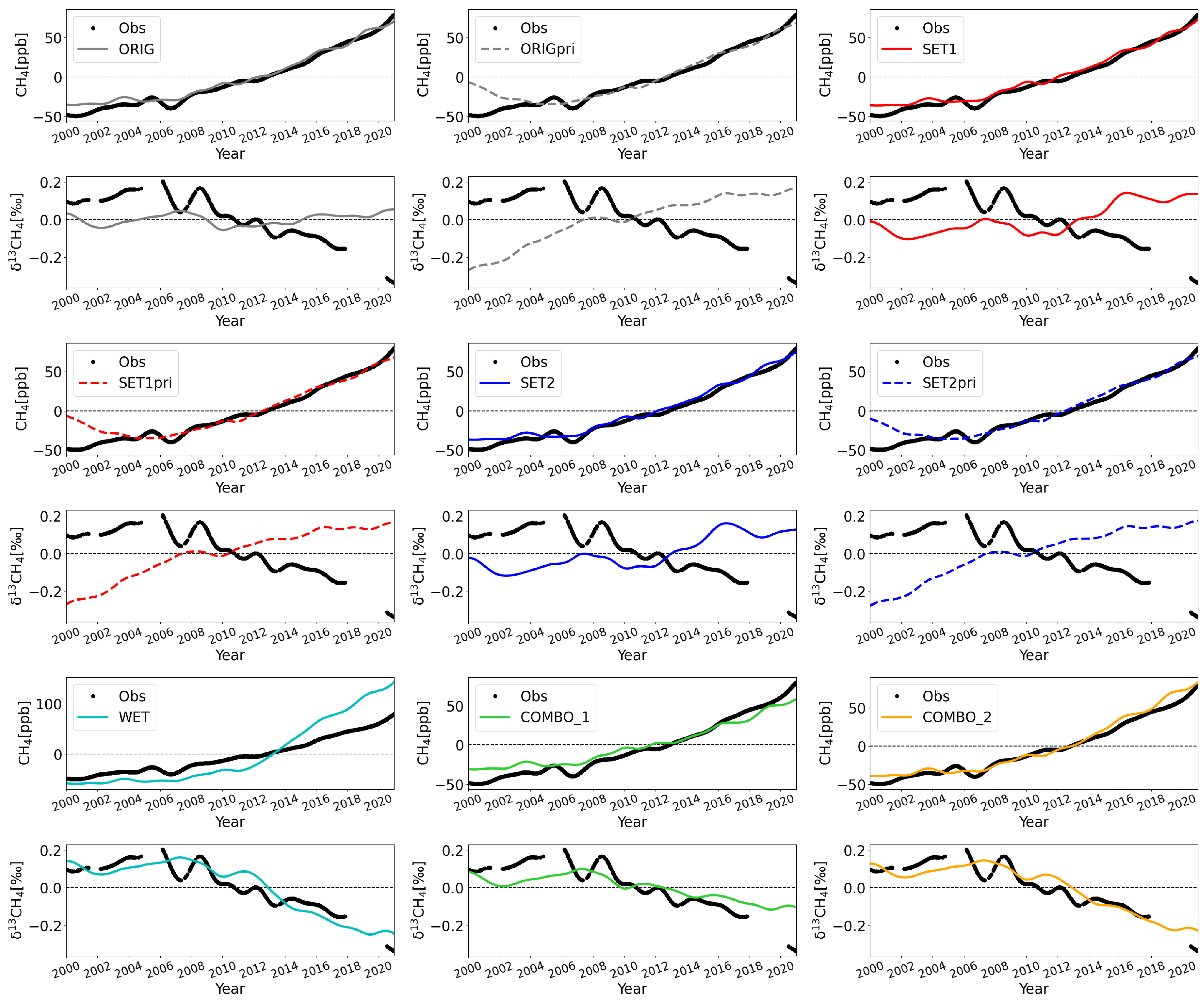
3.2. Estimated CH and CH Trends
4. Discussion
5. Conclusions
Supplementary Materials
Author Contributions
Funding
Institutional Review Board Statement
Informed Consent Statement
Data Availability Statement
Acknowledgments
Conflicts of Interest
Abbreviations
| CTE-CHCH | CarbonTracker-Europe-CH |
| EnKF | Ensemble Kalman Filter |
| ECMWF | European Centre for Medium-Range Weather Forecasts |
| KIE | Kinetic isotopic effect |
| EDGAR | Emissions Database for Global Atmospheric Research |
| LWW | Landfills and waste water treatment |
| EFMM | Enteric Fermentation and Manure Managemnt |
| GFED | Global Fire Emissions Database |
| IPCC | Intergovernmental Panel on Climate Change |
| NOAA/GML | National Oceanic and Atmospheric Administration Global Monitoring Laboratory |
| INSTAAR | Institute of Arctic and Alpine Research |
| BRW | Barrow |
| MHD | Mace Head |
| NWR | Niwot Ridge |
| SPO | South Pole |
References
- Saunois, M.; Stavert, A.R.; Poulter, B.; Bousquet, P.; Canadell, J.G.; Jackson, R.B.; Raymond, P.A.; Dlugokencky, E.J.; Houweling, S.; Patra, P.K.; et al. The Global Methane Budget 2000–2017. Earth Syst. Sci. Data 2020, 12, 1561–1623. [Google Scholar] [CrossRef]
- Bergamaschi, P.; Karstens, U.; Manning, A.J.; Saunois, M.; Tsuruta, A.; Berchet, A.; Vermeulen, A.T.; Arnold, T.; Janssens-Maenhout, G.; Hammer, S.; et al. Inverse modelling of European CH4 emissions during 2006–2012 using different inverse models and reassessed atmospheric observations. Atmos. Chem. Phys. 2018, 18, 901–920. [Google Scholar] [CrossRef] [Green Version]
- Tsuruta, A.; Aalto, T.; Backman, L.; Krol, M.C.; Peters, W.; Lienert, S.; Joos, F.; Miller, P.A.; Zhang, W.; Laurila, T.; et al. Methane budget estimates in Finland from the CarbonTracker Europe-CH4 data assimilation system. Tellus B Chem. Phys. Meteorol. 2019, 71, 1565030. [Google Scholar] [CrossRef] [Green Version]
- Dlugokencky, E.J.; Nisbet, E.G.; Fisher, R.; Lowry, D. Global atmospheric methane: Budget, changes and dangers. Philos. Trans. R. Soc. A Math. Phys. Eng. Sci. 2011, 369, 2058–2072. [Google Scholar] [CrossRef] [PubMed] [Green Version]
- Nisbet, E.G.; Dlugokencky, E.J.; Manning, M.R.; Lowry, D.; Fisher, R.E.; France, J.L.; Michel, S.E.; Miller, J.B.; White, J.W.C.; Vaughn, B.; et al. Rising atmospheric methane: 2007–2014 growth and isotopic shift. Glob. Biogeochem. Cycles 2016, 30, 1356–1370. [Google Scholar] [CrossRef] [Green Version]
- Sherwood, O.A.; Schwietzke, S.; Arling, V.A.; Etiope, G. Global Inventory of Gas Geochemistry Data from Fossil Fuel, Microbial and Burning Sources, version 2017. Earth Syst. Sci. Data 2017, 9, 639–656. [Google Scholar] [CrossRef] [Green Version]
- Schwietzke, S.; Sherwood, O.A.; Bruhwiler, L.M.P.; Miller, J.B.; Etiope, G.; Dlugokencky, E.J.; Michel, S.E.; Arling, V.A.; Vaughn, B.H.; White, J.W.C.; et al. Upward revision of global fossil fuel methane emissions based on isotope database. Nature 2016, 538, 88–91. [Google Scholar] [CrossRef]
- Ganesan, A.L.; Stell, A.C.; Gedney, N.; Comyn-Platt, E.; Hayman, G.; Rigby, M.; Poulter, B.; Hornibrook, E.R.C. Spatially Resolved Isotopic Source Signatures of Wetland Methane Emissions. Geophys. Res. Lett. 2018, 45, 3737–3745. [Google Scholar] [CrossRef]
- Feinberg, A.I.; Coulon, A.; Stenke, A.; Schwietzke, S.; Peter, T. Isotopic source signatures: Impact of regional variability on the δ13CH4 trend and spatial distribution. Atmos. Environ. 2018, 174, 99–111. [Google Scholar] [CrossRef]
- Etiope, G.; Ciotoli, G.; Schwietzke, S.; Schoell, M. Gridded maps of geological methane emissions and their isotopic signature. Earth Syst. Sci. Data 2019, 11, 1–22. [Google Scholar] [CrossRef] [Green Version]
- Brownlow, R.; Lowry, D.; Fisher, R.E.; France, J.L.; Lanoisellé, M.; White, B.; Wooster, M.J.; Zhang, T.; Nisbet, E.G. Isotopic Ratios of Tropical Methane Emissions by Atmospheric Measurement: Tropical Methane δ13 C Source Signatures. Glob. Biogeochem. Cycles 2017, 31, 1408–1419. [Google Scholar] [CrossRef] [Green Version]
- Houweling, S.; Krol, M.; Bergamaschi, P.; Frankenberg, C.; Dlugokencky, E.J.; Morino, I.; Notholt, J.; Sherlock, V.; Wunch, D.; Beck, V.; et al. A multi-year methane inversion using SCIAMACHY, accounting for systematic errors using TCCON measurements. Atmos. Chem. Phys. 2014, 14, 3991–4012. [Google Scholar] [CrossRef] [Green Version]
- Thompson, R.L.; Nisbet, E.G.; Pisso, I.; Stohl, A.; Blake, D.; Dlugokencky, E.J.; Helmig, D.; White, J.W.C. Variability in Atmospheric Methane from Fossil Fuel and Microbial Sources Over the Last Three Decades. Geophys. Res. Lett. 2018, 45, 11499–11508. [Google Scholar] [CrossRef] [Green Version]
- Monteil, G.; Houweling, S.; Dlugockenky, E.J.; Maenhout, G.; Vaughn, B.H.; White, J.W.C.; Rockmann, T. Interpreting methane variations in the past two decades using measurements of CH4 mixing ratio and isotopic composition. Atmos. Chem. Phys. 2011, 11, 9141–9153. [Google Scholar] [CrossRef] [Green Version]
- Lan, X.; Basu, S.; Schwietzke, S.; Bruhwiler, L.M.P.; Dlugokencky, E.J.; Michel, S.E.; Sherwood, O.A.; Tans, P.P.; Thoning, K.; Etiope, G.; et al. Improved Constraints on Global Methane Emissions and Sinks Using δ13C-CH4. Glob. Biogeochem. Cycles 2021, 35, e2021GB007000. [Google Scholar] [CrossRef]
- Saueressig, G.; Crowley, J.N.; Bergamaschi, P.; Brühl, C.; Brenninkmeijer, C.A.M.; Fischer, H. Carbon 13 and D kinetic isotope effects in the reactions of CH4 with O(1D) and OH: New laboratory measurements and their implications for the isotopic composition of stratospheric methane. J. Geophys. Res. Atmos. 2001, 106, 23127–23138. [Google Scholar] [CrossRef]
- Cantrell, C.A.; Shetter, R.E.; McDaniel, A.H.; Calvert, J.G.; Davidson, J.A.; Lowe, D.C.; Tyler, S.C.; Cicerone, R.J.; Greenberg, J.P. Carbon kinetic isotope effect in the oxidation of methane by the hydroxyl radical. J. Geophys. Res. Atmos. 1990, 95, 22455–22462. [Google Scholar] [CrossRef] [Green Version]
- Allan, W.; Struthers, H.; Lowe, D.C. Methane carbon isotope effects caused by atomic chlorine in the marine boundary layer: Global model results compared with Southern Hemisphere measurements. J. Geophys. Res. Atmos. 2007, 112, D04306. [Google Scholar] [CrossRef]
- Hossaini, R.; Chipperfield, M.P.; Saiz-Lopez, A.; Fernandez, R.; Monks, S.; Feng, W.; Brauer, P.; Glasow, R.v. A global model of tropospheric chlorine chemistry: Organic versus inorganic sources and impact on methane oxidation. J. Geophys. Res. Atmos. 2016, 121, 14271–14297. [Google Scholar] [CrossRef] [Green Version]
- Gromov, S.; Brenninkmeijer, C.A.M.; Jöckel, P. A very limited role of tropospheric chlorine as a sink of the greenhouse gas methane. Atmos. Chem. Phys. 2018, 18, 9831–9843. [Google Scholar] [CrossRef] [Green Version]
- Lassey, K.; Ragnauth, S. Balancing the global methane budget: Constraints imposed by isotopes and anthropogenic emission inventories. J. Integr. Environ. Sci. 2010, 7, 97–107. [Google Scholar] [CrossRef] [Green Version]
- Zhang, Y.; Jacob, D.J.; Lu, X.; Maasakkers, J.D.; Scarpelli, T.R.; Sheng, J.X.; Shen, L.; Qu, Z.; Sulprizio, M.P.; Chang, J.; et al. Attribution of the accelerating increase in atmospheric methane during 2010–2018 by inverse analysis of GOSAT observations. Atmos. Chem. Phys. 2021, 21, 3643–3666. [Google Scholar] [CrossRef]
- Milkov, A.V.; Schwietzke, S.; Allen, G.; Sherwood, O.A.; Etiope, G. Using global isotopic data to constrain the role of shale gas production in recent increases in atmospheric methane. Sci. Rep. 2020, 10, 4199. [Google Scholar] [CrossRef] [Green Version]
- Yin, Y.; Chevallier, F.; Ciais, P.; Bousquet, P.; Saunois, M.; Zheng, B.; Worden, J.; Bloom, A.A.; Parker, R.J.; Jacob, D.J.; et al. Accelerating methane growth rate from 2010 to 2017: Leading contributions from the tropics and East Asia. Atmos. Chem. Phys. 2021, 21, 12631–12647. [Google Scholar] [CrossRef]
- Schaefer, H.; Fletcher, S.E.M.; Veidt, C.; Lassey, K.R.; Brailsford, G.W.; Bromley, T.M.; Dlugokencky, E.J.; Michel, S.E.; Miller, J.B.; Levin, I.; et al. A 21st-century shift from fossil-fuel to biogenic methane emissions indicated by 13CH4. Science 2016, 352, 80–84. [Google Scholar] [CrossRef] [PubMed]
- Fujita, R.; Morimoto, S.; Maksyutov, S.; Kim, H.S.; Arshinov, M.; Brailsford, G.; Aoki, S.; Nakazawa, T. Global and Regional CH4 Emissions for 1995–2013 Derived From Atmospheric CH4, δ13C-CH4, and δD-CH4 Observations and a Chemical Transport Model. J. Geophys. Res. Atmos. 2020, 125, e2020JD032903. [Google Scholar] [CrossRef]
- Zhang, Z.; Poulter, B.; Knox, S.; Stavert, A.; McNicol, G.; Fluet-Chouinard, E.; Feinberg, A.; Zhao, Y.; Bousquet, P.; Canadell, J.G.; et al. Anthropogenic emission is the main contributor to the rise of atmospheric methane during 1993–2017. Natl. Sci. Rev. 2021, 9, nwab200. [Google Scholar] [CrossRef]
- Bousquet, P.; Ringeval, B.; Pison, I.; Dlugokencky, E.J.; Brunke, E.G.; Carouge, C.; Chevallier, F.; Fortems-Cheiney, A.; Frankenberg, C.; Hauglustaine, D.A.; et al. Source attribution of the changes in atmospheric methane for 2006–2008. Atmos. Chem. Phys. 2011, 11, 3689–3700. [Google Scholar] [CrossRef] [Green Version]
- Dlugokencky, E.J.; Bruhwiler, L.; White, J.W.C.; Emmons, L.K.; Novelli, P.C.; Montzka, S.A.; Masarie, K.A.; Lang, P.M.; Crotwell, A.M.; Miller, J.B.; et al. Observational constraints on recent increases in the atmospheric CH4 burden. Geophys. Res. Lett. 2009, 36, L18803. [Google Scholar] [CrossRef] [Green Version]
- Tsuruta, A.; Aalto, T.; Backman, L.; Hakkarainen, J.; Laan-Luijkx, I.T.v.d.; Krol, M.C.; Spahni, R.; Houweling, S.; Laine, M.; Dlugokencky, E.; et al. Global methane emission estimates for 2000–2012 from CarbonTracker Europe-CH4 v1.0. Geosci. Model Dev. 2017, 10, 1261–1289. [Google Scholar] [CrossRef] [Green Version]
- Bergamaschi, P.; Segers, A.; Brunner, D.; Haussaire, J.M.; Henne, S.; Ramonet, M.; Arnold, T.; Biermann, T.; Chen, H.; Conil, S.; et al. High-resolution inverse modelling of European CH4 emissions using the novel FLEXPART-COSMO TM5 4DVAR inverse modelling system. Atmos. Chem. Phys. 2022, 22, 13243–13268. [Google Scholar] [CrossRef]
- Peters, W.; Miller, J.B.; Whitaker, J.; Denning, A.S.; Hirsch, A.; Krol, M.C.; Zupanski, D.; Bruhwiler, L.; Tans, P.P. An ensemble data assimilation system to estimate CO2 surface fluxes from atmospheric trace gas observations. J. Geophys. Res. Atmos. 2005, 110, D24304. [Google Scholar] [CrossRef] [Green Version]
- Van der Laan-Luijkx, I.T.; van der Velde, I.R.; van der Veen, E.; Tsuruta, A.; Stanislawska, K.; Babenhauserheide, A.; Zhang, H.F.; Liu, Y.; He, W.; Chen, H.; et al. The CarbonTracker Data Assimilation Shell (CTDAS) v1.0: Implementation and global carbon balance 2001–2015. Geosci. Model Dev. 2017, 10, 2785–2800. [Google Scholar] [CrossRef] [Green Version]
- Krol, M.; Houweling, S.; Bregman, B.; Broek, M.v.d.; Segers, A.; Velthoven, P.v.; Peters, W.; Dentener, F.; Bergamaschi, P. The two-way nested global chemistry-transport zoom model TM5: Algorithm and applications. Atmos. Chem. Phys. 2005, 5, 417–432. [Google Scholar] [CrossRef] [Green Version]
- Tenkanen, M.; Tsuruta, A.; Rautiainen, K.; Kangasaho, V.; Ellul, R.; Aalto, T. Utilizing Earth Observations of Soil Freeze/Thaw Data and Atmospheric Concentrations to Estimate Cold Season Methane Emissions in the Northern High Latitudes. Remote Sens. 2021, 13, 5059. [Google Scholar] [CrossRef]
- Spivakovsky, C.M.; Logan, J.A.; Montzka, S.A.; Balkanski, Y.J.; Foreman-Fowler, M.; Jones, D.B.A.; Horowitz, L.W.; Fusco, A.C.; Brenninkmeijer, C.a.M.; Prather, M.J.; et al. Three-dimensional climatological distribution of tropospheric OH: Update and evaluation. J. Geophys. Res. Atmos. 2000, 105, 8931–8980. [Google Scholar] [CrossRef]
- Huijnen, V.; Williams, J.; van Weele, M.; van Noije, T.; Krol, M.; Dentener, F.; Segers, A.; Houweling, S.; Peters, W.; de Laat, J.; et al. The global chemistry transport model TM5: Description and evaluation of the tropospheric chemistry version 3.0. Geosci. Model Dev. 2010, 3, 445–473. [Google Scholar] [CrossRef] [Green Version]
- Jöckel, P.; Tost, H.; Pozzer, A.; Brühl, C.; Buchholz, J.; Ganzeveld, L.; Hoor, P.; Kerkweg, A.; Lawrence, M.n.G. The atmospheric chemistry general circulation model ECHAM5/MESSy1: Consistent simulation of ozone from the surface to the mesosphere. Atmos. Chem. Phys. 2006, 6, 5067–5104. [Google Scholar] [CrossRef] [Green Version]
- Zhao, Y.; Saunois, M.; Bousquet, P.; Lin, X.; Berchet, A.; Hegglin, M.I.; Canadell, J.G.; Jackson, R.B.; Hauglustaine, D.A.; Szopa, S.; et al. Inter-model comparison of global hydroxyl radical (OH) distributions and their impact on atmospheric methane over the 2000–2016 period. Atmos. Chem. Phys. 2019, 19, 13701–13723. [Google Scholar] [CrossRef] [Green Version]
- Turner, A.J.; Frankenberg, C.; Kort, E.A. Interpreting contemporary trends in atmospheric methane. Proc. Natl. Acad. Sci. USA 2019, 116, 2805–2813. [Google Scholar] [CrossRef] [Green Version]
- Rowlinson, M.J.; Rap, A.; Arnold, S.R.; Pope, R.J.; Chipperfield, M.P.; McNorton, J.; Forster, P.; Gordon, H.; Pringle, K.J.; Feng, W.; et al. Impact of El Niño–Southern Oscillation on the interannual variability of methane and tropospheric ozone. Atmos. Chem. Phys. 2019, 19, 8669–8686. [Google Scholar] [CrossRef] [Green Version]
- Crowley, J.N.; Saueressig, G.; Bergamaschi, P.; Fischer, H.; Harris, G.W. Carbon kinetic isotope effect in the reaction CH4+Cl: A relative rate study using FTIR spectroscopy. Chem. Phys. Lett. 1999, 303, 268–274. [Google Scholar] [CrossRef] [Green Version]
- Spahni, R.; Wania, R.; Neef, L.; van Weele, M.; Pison, I.; Bousquet, P.; Frankenberg, C.; Foster, P.N.; Joos, F.; Prentice, I.C.; et al. Constraining global methane emissions and uptake by ecosystems. Biogeosciences 2011, 8, 1643–1665. [Google Scholar] [CrossRef] [Green Version]
- Kangasaho, V.; Tsuruta, A.; Backman, L.; Mäkinen, P.; Houweling, S.; Segers, A.; Krol, M.; Dlugokencky, E.J.; Michel, S.; White, J.W.C.; et al. The Role of Emission Sources and Atmospheric Sink in the Seasonal Cycle of CH4 and δ;13-CH4: Analysis Based on the Atmospheric Chemistry Transport Model TM5. Atmosphere 2022, 13, 888. [Google Scholar] [CrossRef]
- Snover, A.K.; Quay, P.D. Hydrogen and carbon kinetic isotope effects during soil uptake of atmospheric methane. Glob. Biogeochem. Cycles 2000, 14, 25–39. [Google Scholar] [CrossRef]
- De Laeter, J.R.; Böhlke, J.K.; Bièvre, P.D.; Hidaka, H.; Peiser, H.S.; Rosman, K.J.R.; Taylor, P.D.P. Atomic weights of the elements. Review 2000 (IUPAC Technical Report). Pure Appl. Chem. 2003, 75, 683–800. [Google Scholar] [CrossRef]
- Janssens-Maenhout, G.; Crippa, M.; Guizzardi, D.; Muntean, M.; Schaaf, E.; Dentener, F.; Bergamaschi, P.; Pagliari, V.; Olivier, J.G.J.; Peters, J.A.H.W.; et al. EDGAR v4.3.2 Global Atlas of the three major greenhouse gas emissions for the period 1970–2012. Earth Syst. Sci. Data 2019, 11, 959–1002. [Google Scholar] [CrossRef] [Green Version]
- Crippa, M.; Solazzo, E.; Huang, G.; Guizzardi, D.; Koffi, E.; Muntean, M.; Schieberle, C.; Friedrich, R.; Janssens-Maenhout, G. High resolution temporal profiles in the Emissions Database for Global Atmospheric Research. Sci. Data 2020, 7, 121. [Google Scholar] [CrossRef] [Green Version]
- Giglio, L.; Randerson, J.T.; van der Werf, G.R. Analysis of daily, monthly, and annual burned area using the fourth-generation global fire emissions database (GFED4). J. Geophys. Res. Biogeosci. 2013, 118, 317–328. [Google Scholar] [CrossRef] [Green Version]
- Weber, T.; Wiseman, N.A.; Kock, A. Global ocean methane emissions dominated by shallow coastal waters. Nat. Commun. 2019, 10, 4584. [Google Scholar] [CrossRef] [Green Version]
- Contribution of Working Group I to the Sixth Assessment Report of the Intergovernmental Panel on Climate Change. In Climate Change 2021: The Physical Science Basis; Masson-Delmotte, V.; Zhai, P.; Pirani, A.; Connors, S.; Péan, C.; Berger, S.; Caud, N.; Chen, Y.; Goldfarb, L.; Gomis, M.; et al. (Eds.) Cambridge University Press: Cambridge, UK; New York, NY, USA, 2021. [Google Scholar] [CrossRef]
- Schuldt, K.N.; Aalto, T.; Andrews, A.; Aoki, S.; Apadula, F.; Arduini, J.; Baier, B.; Bartyzel, J.; Bergamaschi, P.; Biermann, T.; et al. Multi-Laboratory Compilation of Atmospheric Carbon Dioxide Data for the Period 1957–2022: Data Set; NOAA: Boulder, CO, USA, 2022. [Google Scholar] [CrossRef]
- Stable Isotopic Composition of Atmospheric Methane (13C) from the NOAA GML Carbon Cycle Cooperative Global Air Sampling Network, 1998–2021; Version: 2022-12-15, University of Colorado, Institute of Arctic and Alpine Research (INSTAAR) Data Set; NOAA: Boulder, CO, USA, 2021. [CrossRef]
- Guidelines for the Measurement of Methane and Nitrous Oxide and their Quality Assurance; WMO/TD-No. 1478, GAW Report No. 185; WMO: Geneva, Switzerland, 2009.
- Miller, J.B.; Mack, K.A.; Dissly, R.; White, J.W.C.; Dlugokencky, E.J.; Tans, P.P. Development of analytical methods and measurements of 13C/12C in atmospheric CH4 from the NOAA Climate Monitoring and Diagnostics Laboratory Global Air Sampling Network. J. Geophys. Res. Atmos. 2002, 107, ACH 11-1–ACH 11-15. [Google Scholar] [CrossRef]
- Bruhwiler, L.; Dlugokencky, E.; Masarie, K.; Ishizawa, M.; Andrews, A.; Miller, J.; Sweeney, C.; Tans, P.; Worthy, D. CarbonTracker-CH4: An assimilation system for estimating emissions of atmospheric methane. Atmos. Chem. Phys. 2014, 14, 8269–8293. [Google Scholar] [CrossRef] [Green Version]
- Thoning, K.W.; Tans, P.P.; Komhyr, W.D. Atmospheric carbon dioxide at Mauna Loa Observatory: 2. Analysis of the NOAA GMCC data, 1974–1985. J. Geophys. Res. Atmos. 1989, 94, 8549–8565. [Google Scholar] [CrossRef]
- Still, C.J.; Berry, J.A.; Collatz, G.J.; DeFries, R.S. Global distribution of C3 and C4 vegetation: Carbon cycle implications. Glob. Biogeochem. Cycles 2003, 17, 6-1–6-14. [Google Scholar] [CrossRef]
- Sherwood, O.; Schwietzke, S.; Arling, V.; Etiope, G. Global Inventory of Fossil and Non-fossilMethane δ13C Source Signature Measurements for Improved Atmospheric Modeling. Available online: https://gml.noaa.gov/ccgg/arc/index.php?id=134 (accessed on 1 April 2023).
- Bakkaloglu, S.; Lowry, D.; Fisher, R.E.; Menoud, M.; Lanoisellé, M.; Chen, H.; Röckmann, T.; Nisbet, E.G. Stable isotopic signatures of methane from waste sources through atmospheric measurements. Atmos. Environ. 2022, 276, 119021. [Google Scholar] [CrossRef]
- Stavert, A.R.; Saunois, M.; Canadell, J.G.; Poulter, B.; Jackson, R.B.; Regnier, P.; Lauerwald, R.; Raymond, P.A.; Allen, G.H.; Patra, P.K.; et al. Regional trends and drivers of the global methane budget. Glob. Chang. Biol. 2022, 28, 182–200. [Google Scholar] [CrossRef]
- Basu, S.; Lan, X.; Dlugokencky, E.; Michel, S.; Schwietzke, S.; Miller, J.B.; Bruhwiler, L.; Oh, Y.; Tans, P.P.; Apadula, F.; et al. Estimating emissions of methane consistent with atmospheric measurements of methane and δ13C of methane. Atmos. Chem. Phys. 2022, 22, 15351–15377. [Google Scholar] [CrossRef]
- Fisher, R.E.; France, J.L.; Lowry, D.; Lanoisellé, M.; Brownlow, R.; Pyle, J.A.; Cain, M.; Warwick, N.; Skiba, U.M.; Drewer, J.; et al. Measurement of the 13C isotopic signature of methane emissions from northern European wetlands. Glob. Biogeochem. Cycles 2017, 31, 605–623. [Google Scholar] [CrossRef] [Green Version]
- Sriskantharajah, S.; Fisher, R.E.; Lowry, D.; Aalto, T.; Hatakka, J.; Aurela, M.; Laurila, T.; Lohila, A.; Kuitunen, E.; Nisbet, E.G. Stable carbon isotope signatures of methane from a Finnish subarctic wetland. Tellus B Chem. Phys. Meteorol. 2012, 64, 18818. [Google Scholar] [CrossRef]
- Tyler, S.C.; Brailsford, G.W.; Yagi, K.; Minami, K.; Cicerone, R.J. Seasonal variations in methane flux and δl3CH4 values for rice paddies in Japan and their implications. Glob. Biogeochem. Cycles 1994, 8, 1–12. [Google Scholar] [CrossRef] [Green Version]
- Bergamaschi, P. Seasonal variations of stable hydrogen and carbon isotope ratios in methane from a Chinese rice paddy. J. Geophys. Res. Atmos. 1997, 102, 25383–25393. [Google Scholar] [CrossRef]
- Zhang, G.; Ma, J.; Yang, Y.; Yu, H.; Shi, Y.; Xu, H. Variations of Stable Carbon Isotopes of CH4 Emission from Three Typical Rice Fields in China. Pedosphere 2017, 27, 52–64. [Google Scholar] [CrossRef]
- Marik, T.; Fischer, H.; Conen, F.; Smith, K. Seasonal variations in stable carbon and hydrogen isotope ratios in methane from rice fields. Glob. Biogeochem. Cycles 2002, 16, 41-1–41-11. [Google Scholar] [CrossRef]
- Zazzeri, G.; Lowry, D.; Fisher, R.E.; France, J.L.; Lanoisellé, M.; Kelly, B.F.J.; Necki, J.M.; Iverach, C.P.; Ginty, E.; Zimnoch, M.; et al. Carbon isotopic signature of coal-derived methane emissions to the atmosphere: From coalification to alteration. Atmos. Chem. Phys. 2016, 16, 13669–13680. [Google Scholar] [CrossRef] [Green Version]
- Liu, Y.; Liang, F.; Shang, F.; Wang, Y.; Zhang, Q.; Shen, Z.; Su, C. Carbon isotope fractionation during shale gas release: Experimental results and molecular modeling of mechanisms. Gas Sci. Eng. 2023, 113, 204962. [Google Scholar] [CrossRef]
- Chang, J.; Peng, S.; Ciais, P.; Saunois, M.; Dangal, S.R.S.; Herrero, M.; Havlík, P.; Tian, H.; Bousquet, P. Revisiting enteric methane emissions from domestic ruminants and their δ 13 C CH4 source signature. Nat. Commun. 2019, 10, 3420. [Google Scholar] [CrossRef] [Green Version]
- Oh, Y.; Zhuang, Q.; Welp, L.R.; Liu, L.; Lan, X.; Basu, S.; Dlugokencky, E.J.; Bruhwiler, L.; Miller, J.B.; Michel, S.E.; et al. Improved global wetland carbon isotopic signatures support post-2006 microbial methane emission increase. Commun. Earth Environ. 2022, 3, 159. [Google Scholar] [CrossRef]
- Takriti, M.; Ward, S.E.; Wynn, P.M.; McNamara, N.P. Isotopic characterisation and mobile detection of methane emissions in a heterogeneous UK landscape. Atmos. Environ. 2023, 305, 119774. [Google Scholar] [CrossRef]


| Station | Station Code | Country | Latitude | Longitude | Elevation [m a.s.l.] | Intake Height [m a. g.] |
|---|---|---|---|---|---|---|
| Barrow | BRW | Alaska, USA | 71.32° N | 156.61° W | 11.00 | 5–16.5 |
| Mace Head | MHD | Ireland | 53.33° N | 9.9° W | 5.00 | 21 |
| Niwot Ridge | NWR | Colorado, USA | 40.05° N | 105.59° W | 3526 | 3 |
| South Pole | SPO | Antarctica | 89.98° S | 24.8° W | 2821.3 | 3–11.3 |
| Emission Source | Signature Value (‰) | Signature Value (‰) |
|---|---|---|
| (Used in This Study) | [14] | |
| Enteric Fermentation and Manure Management (EFMM) | [−67.9,−54.5] 1, −66.8 2 | −62 |
| Landfills and Waste Water Treatment (LWW) | −55.6 2 | −55 |
| Rice (RICE) | −62.1 2 | −63 |
| Coal | [−64.1, −36.1] 1, −40 2 | −35 |
| Oil and Gas | [−56.6, −29.1] 1, −40 2 | −40 |
| Residential | −40 2 | −38 |
| Wetlands | [−74.9, −50] 3, −61.3 2 | −59 |
| Fires | [−25, −12] 1, −22.2 | −21.8 |
| Ocean | −47 2 | −59 |
| Termites | −65.2 2 | −57 |
| Geological | [−68, −24.3] , −40 2 | −40 |
| Simulation | Optimised (categ1) | Optimised (categ2) | Not Optimised (categ3) |
|---|---|---|---|
| ORIG | coal | wetlands | geological |
| oil and gas | soil sink | termites | |
| agriculture * | ocean | ||
| residential | |||
| fires | |||
| SET1 | coal | agriculture * | residential |
| oil and gas | soil sink | fires | |
| wetlands | geological | ||
| termites | |||
| ocean | |||
| SET2 | coal | agriculture * | residential |
| oil and gas | fires | ||
| geological | |||
| termites | |||
| ocean | |||
| wetlands | |||
| soil sink |
| Simulation | Emissions | Modifications |
|---|---|---|
| ORIG | ORIG posteriors | |
| ORIGpri | ORIG priors | |
| SET1 | SET1 posteriors | |
| SET1pri | SET1 priors | |
| SET2 | SET2 posteriors | |
| SET2pri | SET2 priors | |
| WET | ORIG posteriors | After 2012: Wetland emissions +29% |
| COMBO_1 | ORIG posteriors | After 2012: Oil and gas, coal and residential −9% |
| EFMM, LWW and Rice +2% | ||
| COMBO_2 | ORIG posteriors | After 2012: Oil and gas, coal and residential −9% |
| EFMM, LWW and Rice +8% |
Disclaimer/Publisher’s Note: The statements, opinions and data contained in all publications are solely those of the individual author(s) and contributor(s) and not of MDPI and/or the editor(s). MDPI and/or the editor(s) disclaim responsibility for any injury to people or property resulting from any ideas, methods, instructions or products referred to in the content. |
© 2023 by the authors. Licensee MDPI, Basel, Switzerland. This article is an open access article distributed under the terms and conditions of the Creative Commons Attribution (CC BY) license (https://creativecommons.org/licenses/by/4.0/).
Share and Cite
Mannisenaho, V.; Tsuruta, A.; Backman, L.; Houweling, S.; Segers, A.; Krol, M.; Saunois, M.; Poulter, B.; Zhang, Z.; Lan, X.; et al. Global Atmospheric δ13CH4 and CH4 Trends for 2000–2020 from the Atmospheric Transport Model TM5 Using CH4 from Carbon Tracker Europe–CH4 Inversions. Atmosphere 2023, 14, 1121. https://doi.org/10.3390/atmos14071121
Mannisenaho V, Tsuruta A, Backman L, Houweling S, Segers A, Krol M, Saunois M, Poulter B, Zhang Z, Lan X, et al. Global Atmospheric δ13CH4 and CH4 Trends for 2000–2020 from the Atmospheric Transport Model TM5 Using CH4 from Carbon Tracker Europe–CH4 Inversions. Atmosphere. 2023; 14(7):1121. https://doi.org/10.3390/atmos14071121
Chicago/Turabian StyleMannisenaho, Vilma, Aki Tsuruta, Leif Backman, Sander Houweling, Arjo Segers, Maarten Krol, Marielle Saunois, Benjamin Poulter, Zhen Zhang, Xin Lan, and et al. 2023. "Global Atmospheric δ13CH4 and CH4 Trends for 2000–2020 from the Atmospheric Transport Model TM5 Using CH4 from Carbon Tracker Europe–CH4 Inversions" Atmosphere 14, no. 7: 1121. https://doi.org/10.3390/atmos14071121