
Classification and Prediction of Nitrogen Dioxide in a Portuguese Air Quality Critical Zone


1
Faculty of Economics, University of Porto, Rua Dr. Roberto Frias N/A, 4200-464 Porto, Portugal
2
Faculty of Engineering, University of Porto, Rua Dr. Roberto Frias N/A, 4200-464 Porto, Portugal
*
Author to whom correspondence should be addressed.
Atmosphere 2022, 13(10), 1672; https://doi.org/10.3390/atmos13101672
Submission received: 10 September 2022
/
Revised: 25 September 2022
/
Accepted: 2 October 2022
/
Published: 13 October 2022
(This article belongs to the Special Issue Air Quality in Spain and the Iberian Peninsula)
Abstract
:This study presents classification and prediction exercises to evaluate the future behavior of nitrogen dioxide in a critical air quality zone located in Portugal using a dataset, the time span of which covers the period between 1 September 2021 and 23 July 2022. Three main results substantiate the importance of this research. First, the classification analysis corroborates the idea of a neutrality principle of road traffic on the target since the respective coefficient is significant, but quantitatively close to zero. This result, which may be the first sign of a paradigm shift regarding the adoption of electric vehicles in addition to reflect the success of previously implemented measures in the city of Lisbon, is reinforced by evidence that the carbon monoxide emitted mostly by diesel vehicles exhibits a significant, negative and permanent effect on satisfying the hourly limit value associated with the target. Second, robustness checks confirm that the period between 8 h and 16 h is particularly remarkable for influencing the target. Finally, the predictive exercise demonstrates that the internationally patented Variable Split Convolutional Attention model has the best predictive performance among several deep learning neural network alternatives. Results indicate that the concentration of nitrogen dioxide is expected to be volatile and only a redundant downward trend is likely to be observed. Therefore, in terms of policy recommendations, additional measures to avoid exceeding the legal nitrogen dioxide ceiling at the local level should be focused on reducing carbon monoxide emissions, rather than just being concerned about halting the intensity of road traffic.
1. Introduction
Air pollution remains the most serious environmental threat in the European Union (EU). According to estimates by the European Environment Agency (EEA), around 400,000 annual premature deaths can be attributed to air pollution in EU Member States, which must guarantee good air quality standards for their citizens. European Green Deal (EGD) and Zero Pollution Action Plan (ZPAP) highlight the importance of reducing air pollution through the implementation of air quality standards enshrined in EU legislation to effectively protect human health and preserve the natural environment. The EU legislation on air quality—Directive 2008/50/EC—leaves to EU Member States the choice of measures to be adopted in order to comply with the limit values set.
1.1. Context
Regarding nitrogen dioxide (NO), which is the target selected for this study, estimates indicate almost 50,000 premature deaths per year in the EU. This air pollutant negatively affects the human health by promoting severe diseases such as asthma and reduced lung function. Air pollution caused by NO is mainly triggered by economic and human activities such as industry. This source of concern is particularly remarkable in the Iberian Peninsula since this European region is characterized by a strong persistence of both types of activities, being the situation more problematic in urban areas.
1.2. Motivation
If the limit values set by EU legislation are exceeded, EU Member States must adopt air quality plans to ensure the application of appropriate measures to reduce as much as possible the period of exceedance. In May 2019, the European Commission (EC) sent Portugal a first letter of formal notice on air quality, followed by a reasoned opinion in February 2020. Since the EC considered that the effort of Portuguese authorities was unsatisfactory and insufficient given the persistence of poor air quality caused by high levels of NO, it decided to bring a legal action against Portugal at the Court of Justice of the EU in 12 November 2021. This fact constitutes the motivation behind the elaboration of this study. In a nutshell, Portugal has recorded continuous exceedances of the annual limit value for NO in three air quality zones:
- 1.
- North Metropolitan Area of Lisbon (MAL) or, similarly, Lisboa Norte in Portuguese;
- 2.
- Coastal Porto or, similarly, Porto Litoral in Portuguese; and
- 3.
- Between Douro and Minho or, equivalently, Entre Douro e Minho in Portuguese.
1.3. Goals and Research Questions
The goal of this study is to develop classification and prediction exercises to evaluate whether Portugal is likely to satisfy the ceiling associated with NO. In order to perform this empirical assessment, we use public metadata from the city of Lisbon. While the target, also known as (a.k.a.) output or dependent variable, corresponds to hourly measurements of NO concentration levels in the atmosphere, input variables (a.k.a. indicators, explanatory variables, regressors or covariates) include
- Other air pollutants, namely:
- 1.
- Particle matter with a diameter of less than 2.5 m (PM);
- 2.
- Particle matter with a diameter of less than 10 m (PM);
- 3.
- Carbon monoxide (CO); and
- 4.
- Ozone (O).
- Information about meteorological conditions, namely:
- 1.
- Hourly measurements of the atmospheric pressure (AP);
- 2.
- Hourly measurements of the relative humidity (RH);
- 3.
- Hourly measurements of the temperature (T);
- 4.
- Hourly measurements of the precipitation (P);
- 5.
- Hourly measurements of the wind intensity (WI);
- 6.
- Hourly measurements of the wind direction (WD); and
- 7.
- Hourly measurements of the ultraviolet index (UVI).
- Information about noise, measured by the equivalent continuous sound level (ECSL); and
- Information about road traffic, measured by the total hourly traffic volume (THTV).
The technical analysis consists of two steps: first, we develop a discrete choice model to perform a classification analysis; thereafter, we build a novel deep learning neural network (DLNN) model designated by Variable Split Convolutional Attention (VSCA) to perform a predictive analysis. Its innovative and unique character is ratified by the World International Patent Organization (WIPO)’s recent concession of an international patent on December 2021 [1]. While the first step is concerned with the interpretation of coefficients and marginal effects on the target by quantifying how a unit change in a given explanatory variable affects the likelihood of satisfying the NO’s legal ceiling, the second step assesses the performance and generalization power of the VSCA model on forecasting the evolution of NO concentration levels in the atmosphere. With that being said, it is consistent to claim that this study provides answers to two research questions:
- 1.
- Which impact in terms of sign and magnitude does each explanatory variable have on the selected target?
- 2.
- Can the internationally patented VSCA model adequately predict the evolution of NO2 in a Portuguese air quality critical zone?
1.4. Literature and Research Hypotheses
Surprisingly, only a limited number of studies has been concerned with the assessment of NO concentration levels in Portugal. Exceptions include [2,3,4,5].
Ref. [2] analyze daily records of hospital admissions due to cardiorespiratory diseases and levels of PM, NO, O, CO, sulfur dioxide (SO) and nitrogen monoxide (NO) between 1999 and 2004 to evaluate the relationship between air pollution and morbidity in Lisbon through generalized additive Poisson regression models, while controlling for temperature, humidity and seasonality. Authors find significant a positive association between CO and NO markers, as well as between CO and cardiocirculatory diseases in all age groups. Ref. [3] study specific measures to reduce NO emissions considering 2010 as the target-year and using The Air Pollution Model (TAPM). Two scenarios were defined and simulated: the benchmark case considers current NO emissions, while the reduction scenario considers re-estimated NO emissions after the implementation of several measures. Results not only demonstrate a decrease of 4–5 g/m in the annual NO levels, but also ensure compliance with the NO annual limit values in 3—out of 5—air quality stations. Ref. [4] assess atmospheric factors responsible for poor air quality, relationships between air pollution and meteorological variables or atmospheric synoptic patterns between 2002 and 2010. Their study finds a link between the interannual variability of daily air quality and interannual variability of circulation weather types (CWTs). In particular, anticyclonic and north CWTs do not prevail during pollution episodes dominated by easterly CWTs. In general, a higher concentration of NO, PM and O occurs with synoptic circulation characterized by an eastern component and advection of dry air masses. Results on the link between CWTs and air quality for Lisbon and Porto urban areas also suggest that air quality regimes tend to be similar for northern and southern regions, with the exception of spring and autumn PM. Ref. [5] inspect the spatial distribution and trends of NO, NO and O concentrations in Portugal between 1995 and 2010 to claim that NO concentrations have a significant decreasing trend in most urban stations, but a decreasing trend in NO is only observed in stations with less influence from emissions of primary NO.
Some studies also evaluate the relationship between NO concentration levels and health-related outcomes. Ref. [6] assess the health risk of polycyclic aromatic hydrocarbons in air to conclude that the estimated values of lifetime lung cancer risks considerably exceeded the regulatory guideline level. Their results also confirm that historical monuments act as passive repositories for air pollutants present in the atmosphere. By focusing on Estarreja, a region belonging to the center of Portugal where a large chemical complex is installed, Ref. [7] measure the individual daily exposure of two different groups to PM and NO. Results indicate that both groups display a high level of exposure variability and, in general, no significant differences are found between the group composed by workers of the chemical complex and the group of general population working in that region. Ref. [8] analyze main causes of death due to diseases of the circulatory and digestive system, respiratory tract and malignant tumors caused by levels of environmental exposure to PM, PM, O, NO and SO based on data collected in 46 Portuguese municipalities between 2010 and 2015 considering both general linear and backward regression models. Results indicate a downward tendency for the air concentration of PM, NO and O, with different patterns in urban, suburban and rural regions. Mortality from main causes has remained constant, except for diseases of the respiratory tract, which increased and sustains a higher preponderance in rural areas. Additionally, it is estimated that 15 deaths per 10,000 inhabitants could have been avoided with a 10 g/m reduction of the atmospheric level of PM and NO. Ref. [9] evaluate the temporal evolution of air quality in Setúbal between 2003 and 2012 by evaluating seasonal trends of PM, PM, O, NO, NO and NO measured in nine monitoring stations. They conclude that the air quality has improved, with a decreasing trend of air pollutant concentration except for O. Nevertheless, the authors emphasize that PM, O and nitrogen oxides do not necessarily comply with requirements imposed by European legislation and reveal that main sources of PM levels are traffic, industry and wood burning. In a study focused on assessing the impact of schools’ indoor air quality on the health condition of school-age children, Ref. [10] identify ventilation issues and indoor pollutant levels that exceed recommended limits. Some of these, even at low exposure levels, are associated with the development of respiratory symptoms. Nevertheless, environment attributes around schools have a statistically significant effect on respiratory improvements. Ref. [11] compare mean levels of air pollutants in 2020 with those measured between 2014 and 2019 to show a significant improvement in air quality, namely regarding PM and NO, which can be attributed to the restriction of anthropogenic activities promoted by the recent pandemic lockdown. Differently, the authors confirm that O levels exhibit the opposite trend. Ref. [12] compare PM, PM, NO, SO and O before, during, and after the lockdown period in Portugal, while considering 2019 as a control year. All 68 Portuguese stations belonging to urban, suburban and rural zones were considered for this purpose. The authors confirm that NO was the most reduced pollutant in 2020, which coincided with the reduction of road traffic. Considering the period 2010–2017, Ref. [13] assesses trends in atmospheric levels of PM, O, NO and SO, and in mortality rates for diabetes, malignant neoplasms and diseases of the respiratory, digestive and circulatory systems, and explores links between exposure to air pollutants and mortality using statistics methods. The authors conclude that, despite an initial downward trend in PM10 and a peak in O levels, fairly constant air pollution levels were observed in Portugal. Moreover, increases in age-adjusted mortality rates were significant for all diseases except diabetes. They also reveal that lower atmospheric levels of pollutants were observed in rural areas when compared to urban areas, except for O. Results also indicate an increase of 0.30% in the mortality rate for diseases of the respiratory, digestive and circulatory systems, and malignant neoplasms combined is expected to hold for a 10 g/m increase in atmospheric levels of PM.
Lastly, from a statistical point of view, emphasis should be given to the study developed by [14], which characterizes the spatial and temporal dynamics of NO concentration levels in Portugal. The dataset is characterized by a high resolution in the temporal dimension and the respective data incorporates multiple recurring patterns in time, according to the authors, due to social habits, anthropogenic activities and meteorological conditions. Their two-stage modelling approach is combined with a bootstrap procedure to assess uncertainty in parameters estimates, produce reliable confidence regions for the space–time dynamics of the target and a satisfactory model in terms of goodness of fit, interpretability, parsimony, forecasting capability and computational costs. After considering the abovementioned literature and the set of objectives that this study pretends to satisfy, six research hypotheses are formulated:
Hypothesis 1 (H1).
Either nonsignificant or neutral effects characterize the relationship between NO and meteorological input variables.
Hypothesis 2 (H2).
O has a negative impact on the selected target.
Hypothesis 3 (H3).
CO has a negative impact on the selected target.
Hypothesis 4 (H4).
CO is more likely to influence the selected target in the period between 8 h and 16 h.
Hypothesis 5 (H5).
A neutrality principle characterizes the relationship between road traffic and NO.
Hypothesis 6 (H6).
NO is expected to exhibit a decreasing trend in the near future.
While H1–H3 ensure a comparison of our results with those observed in previous studies, H4–H6 allow us to improve the state-of-the-art. In particular:
- H4 guarantees that the classification analysis is categorized according to different peak traffic hours and/or time periods;
- H5 tests whether the use of electric vehicles, which are absent of CO emissions, plays a role on influencing NO concentration levels in the atmosphere; and
- H6 ensures a credible prediction of NO in one of the Portuguese cities with the highest level of air pollution caused by this specific pollutant.
1.5. Summary of Results
Main findings can be summarized as follows. First, the classification analysis corroborates the idea of a neutral effect of road traffic on the target since the respective coefficient is significant, but quantitatively close to zero. Since the time span of analysis covers the period between 1 September 2021 and 23 July 2022, this result may be the first sign of a paradigm shift observable in the city of Lisbon regarding the adoption of electric vehicles, in addition to reflect the success of previously implemented measures (e.g., ban the circulation of vehicles registered before the year 2000). This finding is reinforced by the fact that CO has a significant, negative and permanent effect on the target, thereby reflecting that a higher concentration of NO in the atmosphere is more likely to hold with increasing level of CO emissions. Second, robustness checks confirm that:
- 8–16 h is the period where compliance with the NO’s hourly ceiling is most compromised for a given increase in the level of CO emissions;
- Several regularization procedures confirm that the set of input variables used in the benchmark analysis has explanatory power on the target;
- The input-oriented model aimed at minimizing NO emissions, which is solved through several variants of stochastic frontier analysis, confirms the influence and significance of input variables on the target;
- The two-step continual learning approach also validates benchmark findings from a qualitative point of view; and
- Considering multiple scenarios, a variance importance analysis shows that CO unambiguously has the highest relevance on explaining NO concentration levels.
Third, the predictive exercise demonstrates that the internationally patented VSCA model has the best predictive performance among several DLNN alternatives. Results indicate that:
- 1.
- The level of NO concentrations in the atmosphere is expected to be volatile; and
- 2.
- This air pollutant does not have a downward trend in test and/or validation sets.
Therefore, in terms of policy recommendations, one can conclude that additional measures focused on reducing CO emissions in the period 8 h–16 h should be implemented at the local level to avoid surpassing NO’s limit values in the near future. This is not a contradiction, but rather the manifestation that desirable political actions to maximize social welfare should consider environmental conditions faced by local communities.
2. Materials and Methods
2.1. Overview of Atmospheric Pollution Caused by Nitrogen Dioxide
2.1.1. Description
The exposure to high concentrations of NO can be translated into a serious damage to the human health. When oxidized in the atmosphere, it can even produce nitric acid, which is a component that increases the acidity of rain and causes a degradation in the nature and materials due to its corrosive nature. This is, however, an occurrence with little significance in Portugal. The legislation stipulates air quality objectives for the protection of human health. The indicator used is the annual average of NO, which is an aggregated value of the hourly concentration of this air pollutant measured at each station, for comparison with the respective threshold value. The analysis of air quality at each zone is carried out by considering the worst value obtained in the set of stations belonging to each territorial unit. The typology of a measuring station with respect to the environment (i.e., urban, suburban or rural) and influence (i.e., traffic, industrial or background) of its location allows us to identify the nature of emission sources and the magnitude of measured levels. Lastly, it should be highlighted that trend analyses carried out by the Portuguese Environment Agency (APA) rely on the aggregation of average hourly values, depend on the type of station and allow a better elucidation of measures to be adopted to satisfy limit values throughout the national territory. All stations with a measurement efficiency greater than 75% are used, and in the case of stations covered by some indicative evaluation strategy, measurements with efficiency greater than 14% are considered.
2.1.2. Targets
Main objectives established in Portugal are summarized as follows:
- Ensure compliance with objectives established at the EU level in terms of air quality, which aim to avoid and prevent harmful effects of air pollutants on human health and the environment;
- Assess the air quality throughout the national territory, with a special focus on urban centers; and
- Portuguese legislation materialized by Decree-Law No. 102/2010 of 2010 establishes the obligation to preserve air quality in cases where it is good and improve it in other cases; moreover, it imposes two ceilings on NO—hourly limit value (HLV) and annual limit value (ALV)—that cannot be exceed:
- 1.
- HLV (i.e., a limit value for the average hourly concentration of 200 g/m of NO, which must not be exceeded more than 18 times per calendar year); and
- 2.
- ALV (i.e., a limit value for the average annual concentration of NO of 40 g/m).
This study focuses on analyzing the first type of target.
2.1.3. Evolution
Europe. Regarding NO concentration levels in the EU-28, 2000–2017 is a period marked by a reduction of the mean annual concentration of NO in a magnitude of 25% in suburban stations, 28% at road traffic stations, and 34% at both industrial and rural stations. In 2018, the greatest contribution to NO emissions was the transport sector (47%, with 39% of the road transport and 8% of the non-road transport) followed by the energy supply (15%), agriculture (15%) and industry (15%) sectors [15].
Portugal.Figure 1 provides the concentration level of NO in the biennium 2019–2020 for different Portuguese regions. The year 2020 was atypical due to the pandemic effect on air quality, resulting from several periods of confinement that significantly influenced economic activities and mobility in the national territory. In particular, measures imposed during the state of alert and the state of emergency resulted in a strong reduction in emissions of atmospheric pollutants and led to a significant improvement of air quality, especially in large urban areas. This reduction was predominantly felt in the NO, including in Lisbon, Porto and Braga, where the ALV of 40 g/m has been surpassed in previous years. For the first time, there is no exceedance of this ceiling in large agglomerations, with a decrease in levels measured in the North MAL, from 55 g/m in 2019 to 40 g/m in 2020, in Coastal Porto, from 48 g/m in 2019 to 40.5 g/m in 2020 and in Between Douro and Minho, from 57 g/m in 2019 to 32 g/m in 2020. The significant decrease in the average annual concentration in Between Douro and Minho is explained by the fact that the station that determines the exceedance of the AVL was not used in the 2020 assessment due to malfunctions of the equipment. It can also be observed that, in the remaining local administrative units (LAUs), there is a generalized decrease in the magnitude of measured levels. An exception stands out in Coimbra, where there is a slight increase in NO concentration levels compared to 2019, from 15 g /m to 22 g/m. This situation may result from the use, in the 2019 assessment, of the urban background station instead of the usual road traffic station, which was not operational that year due to equipment failure [16].
Figure 2 presents the annual average value of NO concentration levels by type of station in Portugal during the period 2005–2021. It can be observed a reduction of NO concentration levels between 2009 and 2014, but then a slight increase after 2015 [11]. Nevertheless, Figure 2 allows us to identify a trend of decrease, more accentuated after 2017, in road traffic stations where the most significant exposure of the population to this pollutant occurs and a less expressive decrease in background (i.e., urban and suburban) stations from 2018 afterwards. For the remaining typologies, the magnitude of NO concentration levels has been maintained stable over time, with a series break observed in 2020 because of the lockdown, which influenced the normal functioning of the economy and resulted in the improvement of air quality. With respect to the HLV of 200 g/m not being exceeded more than 18 times a year, Ref. [16] confirms that this air quality objective was fully met in all areas of the national territory during the biennium 2019–2020. This fact collapses and, in some sense, it seems to be inconsistent with the legal action taken by the EC against Portugal in 12 November 2021.
2.2. Data
This study uses public metadata related to the monitoring of:
- 1.
- Air quality;
- 2.
- Noise;
- 3.
- Road traffic; and
- 4.
- Meteorological conditions
In the city of Lisbon, which can be freely accessed online at https://dados.cm-lisboa.pt/dataset/monitorizacao-de-parametros-ambientais-da-cidade-de-lisboa (accessed on 25 July 2022). Currently, this LAU maps the municipality in real or close time, at the level of these indicators, in a sensing-as-a-service mode. This innovation, provided by the MEO/Monitar/QART consortium, consists of an installed network that includes 80 stations, each equipped with different sensors, located mostly on public lighting poles. The selection of locations for the installation of sensors aims to monitor the diversity of spaces with different environmental characteristics and represent the entire county with a homogeneous distribution. As a basis, the following criteria were considered:
- A grid with a spacing of 2 × 2 km;
- Inclusion of requirements related to the Sharing Cities project;
- Incorporation of geographical boundaries of each parish and Reduced Emission Zones (REZs);
- Areas with a homogeneous climate response, land use and occupation rate; and
- The road network proximity to sources of pollution.
In general, available values correspond to hourly average data obtained from an arithmetic mean of 4 segments, where each segment contains 15 min of resolution. Exceptions are road traffic values, which result from summing the number of vehicles per hour. This mapping complements the monitoring carried out by the official network of fixed stations under management of the Lisbon and Tagus Valley Regional Coordination and Development Commission (CCDR-LVT) and the Portuguese Institute of the Sea and Atmosphere (IPMA), whose monitored values in real time are displayed in UTC time in autumn-winter periods and UTC + 1 in spring-summer periods, without decimal places, except for indicators T, RH, P, UVI, WI and WD. The present analysis deals with a multivariate time series (MTS) dataset, whose time span covers the period between 1 September 2021 and 23 July 2022. Descriptive statistics of the set of input variables and target are presented in Table 1.
2.3. Preliminary Statistical Tests and Hypotheses Testing
Prior to classification and prediction exercises, several statistical tests are reported in Table 2, Table 3 and Table 4 to obtain a greater sensitivity on data and justify technical options taken to perform subsequent tasks in the most appropriate way from a scientific point of view.
These include the inspection of:
- 1.
- Multicollinearity;
- 2.
- Normality, skewness and kurtosis;
- 3.
- Homoscedasticity;
- 4.
- Autocorrelation or, similarly, serial correlation;
- 5.
- Stationary;
- 6.
- Specification; and
- 7.
- Hypotheses testing.
2.3.1. Multicollinearity
Results show that the mean variable inflation factor (VIF) corresponds to 51.89, which is above the critical value of 5 usually considered for evaluation. Hence, data suffer from multicollinearity in case of nothing being done. However, all VIF values related to each input variable are below the critical threshold with the exception of those representing PM and PM. These input variables exhibit a positive and strong correlation——and, consequently, both must be excluded from classification and prediction exercises to avoid multicollinearity concerns.
2.3.2. Normality, Skewness and Kurtosis
Results indicate for all normality tests. As such, the null hypothesis claiming the presence of normality in errors’ distribution is rejected for a critical p-value of 5%. Similar conclusion holds true for skewness tests. Nevertheless, Cameron–Trivedi’s decomposition to test the zero kurtosis hypothesis has observed p-value of 0.255, which suggests non-worrying differences compared to the representative kurtosis of a normal distribution at the 5% critical significance level. Overall, these results legitimize to reject the null hypothesis that input variables and target are homogeneously distributed at different time-steps, thereby justifying the execution of several feature engineering actions when moving towards the prediction exercise. In particular, Refs. [17,18] highlight the need to normalize data in cases where either inputs have different units of measure or error terms do not follow a normal distribution. Moreover, outliers can affect the learning ability of DLNN models, particularly if data are concentrated in a very small portion of the input range. Since explanatory variables subject to this type of bias may not have a significant impact on the learning and final predictions of DLNN models, Ref. [19] proposes a solution based on feature engineering to mitigate this technical concern. In a nutshell, it consists of applying a bilateral truncation to the MTS problem based on frequency analysis and histogram re-scaling. As such, in this study, DLNN models initially use normalized data for training and testing. After these tasks being executed, data are de-normalized using the inverse function to ensure a more realistic comparison between actual and predictive values of the target under scrutiny.
2.3.3. Homoscedasticity
Both tests reject the null hypothesis of var, with , . Although heteroscedasticity is more common in cross-sectional samples due to the heterogeneity between individuals, it is also observed in MTS problems due to the presence of temporal differences between different observations. Given the detection of heteroscedasticity, its correction is mandatory when running a multiple linear regression model using the Ordinary Least Squares (OLS) method because coefficients remain centric and consistent, but no longer have minimal variance in the class of linear and centric estimators. White’s procedure, while not solving the problem of heteroscedasticity, restores the validity of statistical inference in large samples such as the one considered in this study [20].
2.3.4. Autocorrelation
Autocorrelation (a.k.a. serial correlation) is more common in time series because observations of the same target in successive periods are often influenced by factors that exhibit some persistence over time. Moreover, autocorrelation can also be induced by data manipulation via certain procedures (e.g., deseasonalization). While the Durbin–Watson test checks whether follows a first-order autoregressive process AR(1), the Breusch–Godfrey test generalizes this assessment to check for the presence of a p-order autoregressive process AR(p). Results in both tests reject the null hypothesis claiming the absence of autocorrelation and suggest the presence of positive autocorrelation (i.e., past NO concentration levels positively influence current values). Given the presence of autocorrelation, regression coefficients are centric and consistent, but they no longer have minimum variance in the class of linear and centric estimators. Furthermore, statistical inference conducted in the usual way is not valid because is no longer the correct formula. In fact, this holds true regardless whether the variance and covariance matrix representative of disturbance terms is known or not. The main drawback of using OLS under these conditions is the loss of validity of the statistical inference, which implies the need to obtain another estimator of that restores the validity of the statistical inference.
Knowing that in the presence of autocorrelation, several estimation methods are useful to achieve this end [21]:
- OLS combined with the Newey–West estimator, after [22] proposing a estimator that is consistent in the presence of heteroscedasticity and/or autocorrelation generated by stationary processes and that asymptotically enables the statistical inference conducted from the OLS results; this estimator is based on a function of estimated residuals obtained by OLS and, unlike White’s procedure, takes into account not only sample variances, but also sample covariances;
- First-order generalized least squares (GLS) method, either in GLS (AR(1)) or EGLS (AR(1)) form, respectively depending on whether is known or not; hence, the GLS estimation is equivalent to the OLS estimation of the original model after this being transformed by the first-order generalized difference method;
- Two-step Cochrane–Orcutt method [23] and subsequent extensions where, in first place, the original model is estimated by OLS to obtain the residuals to estimate the equation , to obtain and then, in second place, use this estimate to construct a set of new input variables from which results a transformed model by first differences; and
- Nonlinear least squares (NLS) method, where the minimization condition cannot be obtained analytically, being necessary to resort to a search algorithm that is developed in several iterations, starting with predefined initial values. The search process ends when a certain convergence criterion defined in advance is satisfied.
2.3.5. Stationary
Several stationary tests were executed in addition to Augmented Dickey–Fuller (ADF) tests reported in Table 3, whose results confirm that the dependent variable does not exhibit unit roots being, thus, unnecessary to integrate the target by taking first- or higher-order differences.
2.3.6. Specification
In terms of specification of the regression model, the observed p-value of the Ramsey test is 0.000, thereby implying that the null hypothesis of a correct specification is strongly rejected for a critical significant level of 5%. This result suggests that the specification can be improved by means of including other input variables (e.g., dummy variables with additive and multiplicative effects related to weekly cyclicality) capable of providing additional explanatory power on the target. However, if this action is not performed, then one must introduce some technique that eliminates the need to include these extra covariates. In this study, roll padding is introduced to overcome this source of concern. This mandatory action is justified by the fact that this method is able to capture the cyclicality of data without the need to include dummy variables representing this statistical property. Therefore, taking into account the result highlighted by the Ramsey test according to which additional input variables must be included, the comparison of a restricted model—absent from weekly cycles—with an unrestricted model—which includes weekly cyclicality—allows us to statistically confirm and formally validate the need to include roll padding and, in affirmative case, avoid the need to include additional input variables representative of weekly cyclicality.
2.3.7. Hypotheses Tests
Based on Table 1 and Table 2, the OLS regression model applied to the MTS problem under analysis is formally described as follows:
where corresponds to the coefficient or weight associated with the independent term, whereas corresponds to the coefficient associated with each input variable j, with . The disturbance term is assumed to be independently and identically distributed with zero mean and constant variance if the hypothesis of homoscedasticity is satisfied, which is not the case as confirmed by White and Breusch–Pagan tests. This regression model must be subject to hypotheses testing for single and joint significance of the set of explanatory variables, whose results are displayed in Table 4. It can be concluded that ECSL, AP, RH, T, P, WI and UVI individually and jointly lack statistical significance for a critical p-value of 5% being, thus, excluded. As such, the restrictive model to be used in the classification exercise is given by
where, as explained in Section 2.4.1, the target consists of a dummy variable, whose development is based on observation values of the latent variable .
2.4. Classification Analysis
2.4.1. Benchmark Model
Generically, considering that a certain observation i falls into one of the m possible categories or alternatives that characterize a given target , a multinomial density is formally defined as follows:
where the probability that the observation i belongs to the alternative j corresponds to
so that the usual multiple linear regression equation in convenient notation is given by:
with corresponding to a vector of components 1, , , …, and is a vector of coefficients or weights associated with the independent terms and regressors. In any discrete choice model, the functional form of should be selected and each lies between 0 and 1 such that their sum over j corresponds to 1
The only exception occurs with the linear probability model (LPM) because the respective binomial distribution implies such that . As such, a problem with the LPM is that predicted probabilities may not be limited to even though their sum over j corresponds to 1. Other weaknesses include obtaining constant marginal effects, the fact that the normality hypothesis is not acceptable and the fact that the homoscedasticity hypothesis is not sustainable. Consequently, the LPM is not used with binary outcome data. Instead, a more satisfactory approach to models containing a dichotomous target is to assume that the dependent variable y is the observable manifestation of an unobservable event (a.k.a. latent variable). Therefore, the benchmark analysis of this case study in particular specifies a rule for determining the binary target as a function of the latent variable , which is defined as follows:
such that each measurement only belongs to one of the two possible categories:
- 1 = HLV is satisfied since the observation i stands below the HLV (alternative); or
- 0 = HLV is surpassed and, thus, not satisfied (base category),
which allows the identification of the probability of the HLV being satisfied and quantifying the magnitude of the marginal effect that each regressor has on the target. Obviously, after considering the battery of preliminary statistical tests, the binary regression model can be formally written as follows
where is the disturbance term. In the class of models characterized by the relations (1) and (2), it follows that:
and, by complementarity, also:
Then, being a random variable with a distribution function , yields that
The two most common choices for the functional form of are those corresponding to the logistic distribution (reduced normal distribution) representative of the logit (probit) model, respectively. In the probit model, it is postulated that is the normal distribution function
whose associated probability density function is given by:
In the logit model, the choice of falls onto:
which is the distribution function of a logistic variable with zero mean and variance . The probability density function of the logistic distribution is given by:
It is easy to verify that the equality,
is unequivocally verified. In both cases, predicted probabilities are limited to .
From a theoretical point of view, Ref. [24] confirms that the choice between logit and probit depends on the type of characteristics sustained by the dependent variable. Ref. [25] details that, if the dependent variable is directly observed and measured in reality, then a logit model is expected to be the optimal choice to estimate the probability that a given observation falls into a certain category. Despite these normative considerations, this study follows objective criteria to determine the optimal model, which is the one that exhibits the lowest Akaike information criterion (AIC) and Bayesian Information criterion (BIC) and the highest log-pseudolikelihood.
Estimated coefficients assume the base category as reference point, so that their interpretation is given as follows: compared to the HLV violation scenario, a unit increase in a given explanatory variable makes compliance with the HLV associated with the level of NO concentration in the atmosphere more (less) likely if the respective coefficient takes a positive (negative) sign, respectively.
In turn, the marginal effect of a given regressor on the probability of belonging to the alternative j results from observing
such that
where designates the density function corresponding to the distribution function . In (4), the first member is a column vector of partial derivatives of which the generic component is, assuming that is a linear function of
The sum of marginal effects associated with each category is equal to zero and their interpretation is straightforward: a unit increase in a given explanatory variable either increases or decreases the probability of belonging to alternative j by the magnitude expressed in percentage terms. Additionally, two facts deserve emphasis in (5):
- 1.
- Marginal effects vary across distinct observations given that different explanatory variables influence the probability density function ; and
- 2.
- Marginal effects can vary for a given observation since the magnitude of the effect may be different from one value of to another.
As such, in addition to estimated coefficients, this study reports both marginal effects at the mean and average marginal effects.
2.4.2. Technical Extensions
Several formal extensions are proposed to test whether benchmark findings remain qualitatively robust, namely:
- 1.
- Application of a supervised machine learning (ML) model combined with several regularization methods to the set of inputs used in the classification exercise;
- 2.
- Use of a two-step continual learning (CL) approach;
- 3.
- Execution of a variable importance analysis (VIA);
- 4.
- Evaluation of the ordered multinomial discrete choice model (OM-DCM) by increasing the number of categories that define the target; and
- 5.
- Development of a stochastic frontier analysis (SFA);
Standard regularization. To dissuade concerns related to the omitted variable bias, this robustness check consists of a four-step procedure:
- 1.
- Initially, a supervised ML model—logistic LASSO—is exogenously chosen;
- 2.
- The objective function of this supervised ML model accommodates a penalty component that must be optimized. To achieve this purpose, a certain penalized regression technique (a.k.a. regularization method or tuning process) is applied to the initial set of covariates in order to find the general degree of penalization (a.k.a. penalty level) that optimizes the objective function, which is represented by . After identifying the optimal value of this parameter, one can find which input variables have a statistically significant impact on the target and, for each of these, the weight or coefficient on the target which, similarly to what was verified in the initial exercise, can only be interpreted in terms of sign. In this extension, three regularization techniques are combined with the logistic LASSO model:
- k-fold cross-validation, whose purpose is to assess the out-of-sample classification performance;
- AIC, BIC and Extended Bayesian information criterion (EBIC), by finding the penalty level that corresponds to the lowest value taken by each of these information criteria; and
- Rigorous penalization, which corresponds to a penalty level formally given by , where c is a slack parameter with default value of 1.1, is the standard normal cumulative distribution function (CDF) and is the significance level, whose default value is . According to [26], this approach requires standardized predictors and the penalty level is motivated by self-normalized moderate deviation theory to overrule the noise associated with the data-generating process.
- 3.
- After identifying covariates with explanatory power on the target, coefficients are estimated; and
- 4.
- Although not mandatory because classification metrics (e.g., cross-entropy loss) can be reported, we convert the classification problem into a regression problem in order to run the Wilcoxon signed-rank test and provide the following metrics: RMSE, MAE, Mean Absolute Percentage Error (MAPE) and Theil’s U statistic. The later is a relative accuracy measure that compares the predicted outcomes with results of forecasting with minimal historical data.
Two-step continual learning approach. In alternative to the previous regularization techniques, this study considers a two-step CL model proposed in [27]. In the context of ML, the idea behind CL is to refine the treatment of covariates based on a bias-variance trade-off argument given that CL consists of a two-step procedure where:
- 1.
- In a first step, random forest (RF) is applied to the set of covariates holding a strong relative importance on explaining the dependent variable in order to mitigate the risk of overfitting; and
- 2.
- In a second step, a probit model estimated by the maximum likelihood method is applied to predicted target values obtained in the first step to mitigate the risk of underfitting.
Overall, this approach is justified by the fact that it dissuades concerns related to endogeneity, spurious correlation and reverse causation.
Variable importance analysis. Following [28], VIA is applied to gain additional robustness over the regularization approaches previously considered for variable selection. This way, the analysis provides a tool to assess the importance of input variables when dealing with complex interactions, making the framework more interpretable and computationally more efficient. VIA is performed under four different circumstances:
- Applied to the entire set of input variables;
- Only applied to meteorological data;
- Only applied to ai pollutants; and
- Only applied to statistically significant covariates.
Ordered multinomial discrete choice model. Thenceforth, we decide to increase the number of categories representing the dependent variable, which is now expressed as:
The intermediate category can be interpreted as a class containing observations characterized by a strong sensitivity towards the HLV of NO. From a theoretical point of view, multinomial logit models are used for discrete outcome modeling by operating under a logistic distribution being, thus, preferred for large samples. Probit models operate differently for a dependent variable defined by more than two categories, particularly when these obey to a ranking. In MTS problems, Ref. [29] find evidence that the logit specification provides a better fit in the presence of independent variables that exhibit extreme levels. Conversely, model fit with random effects in moderate size datasets is improved by selecting a probit specification. Notwithstanding, in similar vein to the benchmark exercise, this extension uses statistical criteria to decide between using logit and probit multinomial models. However, only the ordered form is considered in this extension given that, ceteris paribus, any municipality unequivocally prefers to observe a low level of NO concentrations in the atmosphere.
Stochastic frontier analysis. Lastly, the benchmark exercise is complemented by the inclusion of an input-oriented SFA based on the ground that a policymaker pretends to minimize the latent output variable NO (i.e., concentration level of NO in the atmosphere) given the set of input variables.
2.4.3. Normative Improvements through Sample Segmentation
The initial assessment is also improved by developing three normative extensions based on a segmentation according to:
- 1.
- Peak traffic hours (8 h–16 h, 16 h–24 h and 24 h–8 h);
- 2.
- Seasons (summer, spring, autumn and winter); and
- 3.
- The weekend–weekdays dichotomy.
2.5. Prediction Analysis
Framework
Feature engineering. DLNN models are trained, tested and validated by considering a 50-25-25 partition. This rule ensures a prediction of NO concentration levels for 81 days ahead in the test and/or validation set. As required in MTS problems, shuffling is neglected [30]. Figure 3 clarifies that the set of DLNN models used in this study define a time resolution of inputs (outputs) in hours (days), respectively. In particular, 168 time-step hours correspond to the resolution used for input variables, while the output to be predicted corresponds to the average of the next 24 time-step hours. As such, the predictive exercise considers historical data corresponding to one week in order to predict the average level of NO concentrations in the atmosphere during 24 h, representative of the first day of the following week. In addition to the subset of covariates previously identified as being statistically significant through the application of Wald tests in Section 2.3 (i.e., O, CO, THTV and WD), three additional regressors are included in the set of input variables adopted for the prediction exercise:
- 1.
- AP because the respective Wald test indicates that this covariate is statistically significant for a critical p-value of 10% when NO residuals follow a logistic distribution, which corresponds to the inclusion of a softmax layer in DLNN frameworks;
- 2.
- The target lagged in time by one period, , based on the presence of autocorrelation identified by Durbin–Watson, Breusch–Godfrey and autoregressive conditional heteroscedasticity (ARCH) tests; and
- 3.
- ECSL, which is not individually significant according to the Wald test, so that the DLNN models used in the prediction exercise are expected to assign a null weight to this input variable; hence, its inclusion is justified by the need to identify the consistency between the statistical robustness associated with the pre-processing phase and the set of different DLNN models used in the forecast analysis.
Thus, as shown in Figure 3, a total of 7 input variables are used in the prediction exercise.
Benchmark models. To evaluate and compare the performance of the proposed DL innovative model, we consider the following benchmark models:
- WaveNet defined by [31], where the application of a grid search to find its optimal depth shows that this is given by . A relevant aspect from this model is the use of causal convolutions, which ensures that the order of data modeling is not violated. Hence, the prediction generated by the WaveNet at time-step cannot depend on future time-steps. Another key characteristic is the use of dilated convolutions to gradually increase the receptive field. A dilated convolution is a convolution where the kernel K is applied over one area larger than its length k by skipping input values with a certain step. It is equivalent to a convolution with a larger filter derived from the original filter by dilating it with zeros. Hence, when using a dilation rate for any , the causal padding has size given by . Finally, as recognized by [32], the residual block is the heart of a WaveNet, being constituted by two convolutional layers, one using the sigmoid activation function and another using the tanh activation function, which are multiplied by each other. Then, inside the block, the result is pass through into another convolution with and . This technique is referred to as the projection operation or channel pooling layer. Both residual and parametrized skip connections are used throughout the network to accelerate convergence and enable training of much deeper models. This block is executed a given number of times in the depth of the network, with depth}. The dilatation increases exponentially according to the formula .
- Temporal Convolutional Network (TCN) defined by [33], where the application of a grid search allows us to conclude that one should optimally consider , with and a global kernel size given by . The TCN is characterized by three main characteristics:
- -
- Convolutions in the architecture are causal, which means that there is no information moving from future to past since causal convolutions imply that an output at time t is convolved only with elements from time t and earlier (i.e., sequence modeling) from the previous layer;
- -
- The architecture can take an input sequence of any length and map it to an output sequence of the same length similarly to RNNs; hence, similar to the WaveNet model, causal padding of length is added to keep subsequent layers with the same length as previous ones; and
- -
- It is possible to build a long and effective history size using deep neural networks augmented with residual blocks and dilated convolutions.
- Standard Long Short-Term Memory (LSTM) of [34], where the application of a grid search reveals as optimal strategy the inclusion of a first LSTM layer with 64 neurons, input shape of , active return sequences and ReLu activation function, followed by a second LSTM layer with 32 neurons and without active return sequences; these layers are followed by three dense layers, where the last one for the output is defined with tanh activation function; the remaining optimal technical options include 100 epochs with a batch size of 64 and applying the Adam optimizer. Conceptually, the LSTM has three basic requirements:
- -
- The system should store information for arbitrary durations;
- -
- The system should be resistant to noise (i.e., fluctuations of random or irrelevant inputs to predict the correct output); and
- -
- Parameters should be trainable in a reasonable time.
The LSTM adds a cell state c to the standard RNN that runs straight down the entire recursive chain with only some minor linear interactions to control the information that needs to be remembered. These control structures are called gates. Activations are stored in the internal state of an LSTM unit (i.e., recursive neuron), which holds long-term temporal contextual information. A common architecture consist of a memory cell c and its update input gate i, output gate o and forget gate f. Gates have in and out connections. Weights of connections, which need to be learned during training, are used to orient the operation of each gate. - LSTM of [34] complemented by the standard attention mechanism of [35]. A standard attention mechanism is a residual block that multiplies the output with its own input and then reconnects to the main pipeline with a weighted scaled sequence. Scaling parameters are called attention weights and the result is called context weights for each value i of the input sequence. As such, c is the context vector of sequence size n. The computation of results from applying a softmax activation function to the input sequence on layer l, thereby meaning that input values of the sequence compete with each other to receive attention. Knowing that the sum of all values obtained from the softmax activation corresponds to 100%, attention weights in the attention vector have values within .
- Bi-Dimensional Convolutional Long Short-Term Memory (ConvLSTM2D) defined by [36] considering 7 segments, where each segment represents 1 day, each day consists of 24 time-step hours and each time-step corresponds to 1 h. The ConvLSTM2D is a recurrent layer similar to the LSTM, but internal matrix multiplications are exchanged with convolution operations. Since we are dealing with a MTS problem, the concept of sequence segment is introduced to make inputs compatible with ConvLSTM2D layers, which have to deal with segments of temporal sequences. Data flow through the ConvLSTM2D cells by keeping a 3D input dimension composed by Segments × TimeSteps × Variables rather than merely applying a 2D input dimension composed by TimeSteps × Variables as observed in the standard LSTM.
Details on the standard attention mechanism. Attention is a mechanism to be combined with LSTM layers to ensure the focus on certain parts of the input sequence, thereby enabling a higher quality of learning [35]. Attention was originally introduced for machine translation tasks, but it was rapidly spread into many other application fields. As highlighted in Figure 4, the basic attention mechanism can be seen as a residual block that multiplies the output with its own input and then reconnects to the main pipeline with a weighted scaled sequence. Scaling parameters are called attention weights and the result is called context weights for each value i of the input sequence. As such, c is the context vector of sequence size n. Formally
The computation of results from applying a softmax activation function to the input sequence on layer l
which means that input values of the sequence compete with each other to receive attention. Knowing that the sum of all values obtained from the softmax activation is 1, attention weights in the attention vector have values within . Since we are dealing with a MTS problem, Figure 4 shows the incorporation of attention mechanism in a 2D dense layer (i.e., the standard attention mechanism). This layer is subject to a permutation to ensure that the attention mechanism is applied to the time-steps dimension of each sequence and not to the dimension representative of input variables. It is important to highlight that, when the attention mechanism is applied after the LSTM layer, it must return internal generated sequences, which are equal to the number of recursive cells (NRC). This parameter is used inside the attention block to know how many sequences must be processed.
Details on the bi-dimensional convolutional long short-term memory. Ref. [36] propose the ConvLSTM2D layer to predict future rainfall intensity based on sequences of meteorological images. By using this layer in a DLNN model, they were able to outperform state-of-the-art algorithms. The ConvLSTM2D is a recurrent layer similar to the LSTM, but internal matrix multiplications are exchanged with convolution operations. As highlighted in Figure 5, the concept of sequence segment is introduced to make inputs compatible with ConvLSTM2D layers, which in turn deal with segments of temporal sequences in light of the MTS problem under scrutiny.
Data flow through the ConvLSTM2D cells by keeping a 3D input dimension composed of Segments × TimeSteps × Variables rather than just the typical 2D input dimension consisting of TimeSteps × Variables as in the standard LSTM. The ConvLSTM2D model can be useful for the prediction of NO concentration levels because this MTS problem can have certain individual patterns for each day of the week that can be grouped and contained into a 2D input dimension. For this DLNN model in particular, 7 segments were used, where each segment represents 1 day, each day consists of 24 time-steps and each time-step corresponds to 1 h.
Proposed innovative deep learning neural network model. Two improvements are added on top of the ConvLSTM2D model:
- 1.
- Inclusion of convolutional layers inside the attention block to ensure that input variables are split to assess the individual influence of each input variable on the target [1]; and
- 2.
- Incorporation of roll padding, which is a new padding method that allows us to dissuade the specification problem identified by the Ramsey test.
The first technical refinement consists of introducing convolutional layers inside the attention block. Attention mechanisms can be useful to obtain a pattern of attention in contiguous time-steps, particularly in the context of MTS problems. Two types of convolutional layers can be introduced inside any attention block:
- One dimensional (1D) convolutional (i.e., Conv1D) layers; and
- Two dimensional (2D) convolutional (i.e., Conv2D) layers.
The implementation of Conv1D layers inside the attention block requires that, after the multivariate sequence being split by variable, a path should be created for each univariate sequence processed with 1D convolutional layers. It is also important to observe that, inside the attention block, each path must return a 1D vector with size TimeSteps, using only one convolution kernel. Additionally, this single channel 1D convolution output must use the softmax activation. The result of each path is concatenated leading to the formation of a feature map of size TimeSteps × Variables with attention weights for each input variable.
Nevertheless, as observed in Figure 6, the novelty in the proposed architecture consists of introducing Conv2D layers inside the attention block for the ConvLSTM2D model, which deals with 3D maps holding a Segments × TimeSteps × Variables format. After the segmented multivariate sequence being split by variable, a 2D input dimension is formed since the new map is characterized by a Segments × TimeSteps format, which is then processed by 2D convolutional layers. This means that a 2D kernel is not only able to capture patterns in contiguous time-steps, but it also has the ability to identify patterns for the same time-step in previous and next segments (e.g., when a segment represents days and time-steps correspond to hours, a 2D kernel captures patterns that associate different hours of the day i as well as patterns that associate the same hour j in adjacent days to the day i). Note that the 2D output map for each variable is the result of a softmax activation function. Individual values for each explanatory variable in the resulting 2D map compete against each other and their sum is equal to 1 with a scaling factor ranging between . As described in Equation (7), the resulting after all convolutions being concatenated is a compatible 3D map to scale inputs h of the attention block to obtain c.
Figure 6 also reveals that roll padding can be used to complement the Conv2D attention mechanism, particularly in MTS problems that exhibit cyclical properties. Since the analysis deals with segments of 7 days, roll padding can be used in the component representing segments to ensure that the first day of a given week is correlated with the last day of the previous week once assuming that data exhibit a weekly cyclicality. To confirm that this fact holds true in the MTS problem under scrutiny, one needs to compare the unconstrained model given by:
against the restricted model that corresponds to:
by means of performing a likelihood ratio (LR) test to check for the joint significance of the null hypothesis , where corresponds to a dummy variable that represents the first week of each month, corresponds to a dummy variable that represents the second week of each month, corresponds to a dummy variable that represents the third week of each month and corresponds to a dummy variable that represents the fourth week of each month. Note that both models should not include the regression coefficient related to the independent term to ensure that the statistical test confronting both models is focused on capturing significant differences strictly caused by weekly cyclicality. Note that it is mandatory emphasizing that the statistical test must be developed without including the independent term since this action, which consists of creating a regression model with centered explanatory variables, is the correct way to empirically infer the quality adjustment of any regression model because centering a model allows to remove the unobserved–heterogeneous–characteristics affecting the data, so that all regression coefficients remain equal to the original model with the exception of the independent term’s coefficient, which disappears from the orginal model’s specification. If the observed p-value is below the critical significance level of 5%, then the null hypothesis representative of the absence of weekly cyclicality can be rejected. If this statistical property is verified, then we are obliged to introduce dummy variables representing weekly cyclicality or, alternatively, not introduce them through the inclusion of roll padding. Estimated coefficients of the restricted model in (10) are given by:
with = 0.9745, while estimated coefficients of the unrestricted model in (9) that includes additive effects representative of weekly cyclicality correspond to
with = 0.9746, standard errors within parentheses and observed t-statistics within brackets.
The LR test result is , thereby implying that the null hypothesis contemplating the absence of weekly cyclicality is rejected. Similar conclusion emerges from the Wald test applied to assess the joint significance of all additive effects, given that for the case with uncontrolled heteroscedasticity and for the case with inclusion of robust standard errors by considering the White’s procedure to control for heteroscedasticity.
Individual significance test results also indicate that each dummy variable is relevant to explain the target given that in addition to obtain , and for the case with uncontrolled heteroscedasticity and, for the case with inclusion of robust standard errors to control for heteroscedasticity, yields , , and .
Consequently, knowing that roll padding is a process capable of capturing the 7-days window cyclicity observed in the data, the incorporation of dummy variables D1, D2, D3 and D4 in the set of input variables becomes a redundant action.
For illustrative purposes, Figure 7 describes the ConvLSTM2D architecture with the Conv2D attention mechanism and roll padding, which defines the internationally patented VSCA model.
2.6. Conceptual Framework and Methodological Pipeline
In order to systematize main ideas related to the empirical analysis and robustness checks, Figure 8 presents the conceptual framework—including research hypotheses—and the methodological pipeline adopted in this study.
3. Results
3.1. Classification
3.1.1. Performance, Model Selection, Interpretation of Coefficients and Marginal Effects
Probit and logit exhibit high sensitivity but also low specificity, which suggests that both discrete choice models predominantly fail to predict observations that do not comply with the legal hourly ceiling imposed onto NO concentration levels.
However, as a large part of the sample is composed of observations that satisfy the HLV associated with the target, both models end up showing a good classification capacity, manifested by high accuracy values. Knowing that probit is considered the best binary model since it exhibits the highest log-likelihood and the lowest AIC and BIC, (6) in Table 5 displays key results for clarifying the benefit of this classification analysis. In addition to verifying that all coefficients are significant, the following interpretation can be inferred:
- Negative sign of O and CO indicates that satisfying the HLV of NO is less likely with additional level of O and CO emissions;
- Positive sign of WD reveals that satisfying the HLV of NO is more likely when the wind direction changes from north to east; and
- Even more interestingly, the null value taken by the representative coefficient of THTV suggests that higher road traffic does not influence the fulfilment of NO’s legal hourly ceiling. Consequently, this result allows us to conclude that THTV has a neutral character on satisfying the HLV associated with the target.
Moreover, both types of marginal effects are significant and quantitatively indicate that:
- In average terms, in the set of 7824 observations of the sample, it is estimated that an additional g/m of CO emitted to the atmosphere decreases the probability of satisfying the HLV of NO by 19.1 percentage points (p.p.); however, at the mean observation level, the probability of satisfying the HLV of NO only decreases 2.3 p.p.;
- In average terms, in the set of 7824 observations of the sample, it is estimated that an additional g/m of ozone concentrated in the air decreases the probability of satisfying the HLV of NO by 0.04 p.p. while, at the mean observation level, this probability drops 0.01 p.p.;
- At the level of wind direction, the exact value of the average marginal effect is 0.0000575 which suggests that, for each change in wind direction from north to east in the magnitude of 100 degrees, the probability of satisfying the HLV concentration of NO increases by 0.58 p.p.; at the average observation level, the increase is only 0.07 p.p. given the value 7.02 × 10 taken by the respective marginal effect; and
- With regard to road traffic, the exact value of the average marginal effect is 4.12 × 10, which suggests that, for every 10,000 additional vehicles circulating per hour in the city of Lisbon, the probability of satisfying the HLV of NO concentration decreases by 4.12 p.p.; at the mean observation level, the reduction is only 0.05 p.p. given the value 5.03 × 10 taken by the respective marginal effect.
Considering the set of research hypotheses formulated in Section 1 and relying on the outcomes of this initial classification exercise, it can be stated that:
- H1 and H3 are verified and thus unequivocally validated; notwithstanding, despite the magnitude being low, results indicate that a change in wind direction can influence the probability of satisfying NO’s legal hourly ceiling;
- H2 is only partially verified because, although O negatively influences the probability of compliance with the HLV associated with the target, the magnitude of the effect is redundant; and
- H5 is also ratified such that, during the period between 1 September 2021 and 23 July 2022, results suggest that the relationship between THTV and NO is characterized by the approximation to what, in the absence of a better terminology, can be considered a principle of neutrality.
3.1.2. Standard Regularization Techniques Combined with Logistic LASSO
Table 6 shows results of the logistic LASSO model combined with three different regularization techniques: k-fold cross-validation, rigorous penalization and information criteria (i.e., AIC, BIC and EBIC). This extensions allows us to formulate three main conclusions:
- 1.
- Depending on the penalization technique adopted to reduce input dimensionality, it can be concluded that only AP and WI are included on top of the input variables used in the initial exercise;
- 2.
- Results show that the sign exhibited by the estimated coefficients is coherent across different regularization techniques.; and
- 3.
- More importantly, the sign of each coefficient does not change relative to the benchmark scenario, which qualitatively reinforces the initial findings.
3.1.3. Continual Learning
While the first step of the CL approach allows us to obtain predicted probabilities of the dependent variable by means of applying RF to the set of input variables, the second step uses these values as dependent variable of a binary probit/logit estimation. Estimated coefficients displayed in Table 7 exhibit the same sign to those sustained in the initial classification exercise, thereby confirming the qualitative robustness of benchmark results.
3.1.4. Variable Importance Analysis
VIA is also performed, whose outcomes in Figure 9a–d demonstrate that:
- Regardless of the scenario, CO has the highest relative importance on the target;
- WD has the strongest relative importance on NO if considering only weather conditions; and
- VIA outcomes are clearly consistent with those yielding in the benchmark analysis.
3.1.5. Ordered Multinomial Discrete Choice Model
Coefficients of the logit and probit ordered model differ by a scale factor. Therefore, similarly to the binary DCM, only their sign can be subject to interpretation. Results displayed in Table 8 indicate that the ordered logit model is the optimal choice for assessing coefficients and marginal effects since it exhibits the highest log-likelihood and the lowest information criteria, with AIC of 4040.452 and BIC of 4082.242. All estimated coefficients are statistically significant and their interpretation is straightforward: the reduction of NO is improved—from the worst category with concentration levels above or equal to 250 g/m to the intermediate category with concentration levels between 150 and 249 g/m and the best category with concentration levels below 150 g/m—with decreasing (increasing) CO and O (WD and THTV) values, respectively. Therefore, a first conclusion is that the results of binary and multinomial DCMs are consistent. Moreover, intercept parameters of the OM-DCM are significantly different from each other, which validates the more refined segmentation of the target. Results also show that marginal effects at the mean and average marginal effects from the logit estimation resemble to those of the probit model. A key characteristic of marginal effects is that their sum across categories is necessarily zero.
Consequently, when a certain target is divided in more than two classes, one can identify which category is more volatile to changes in a given regressor. Focusing on the average marginal effect of CO on the target, it can be concluded that:
- With the probit model, one unit increase in CO is associated with being 88.65 p.p. less likely to fall in the category of low NO concentration levels, 87.26 p.p. more likely to stand in the intermediate category of NO concentration levels—where the HLV either may or may not be surpassed—and 1.39 p.p. more likely to be part of the category that largely exceeds the HLV of NO; and
- With the logit model, one unit increase in CO is associated with being 92.28 p.p. less likely to fall in the category of low NO concentration levels, 90.86 p.p. more likely to stand in the intermediate category of NO concentration levels and 1.43 p.p. more likely to be part of the category that largely exceeds the HLV of NO, which implies that the logit estimation sharpens even more the chance of falling into the low or intermediate categories of NO.
Now, focusing on the marginal effect at the mean, it can be observed that:
- With the probit model, one unit increase in CO is associated with being 84.88 p.p. less likely to fall in the category of low NO concentration levels and 84.88 p.p. more likely to stand in the intermediate category of NO concentration levels, while it has a null influence on the likelihood of belonging to the category that largely exceeds the HLV of NO; and
- With the logit model, one unit increase in CO is associated with being 75.99 p.p. less likely to fall in the category of low NO concentration levels and 75.98 p.p. more likely to stand in the intermediate category of NO concentration levels, while it has a null influence on the likelihood of belonging to the category that largely exceeds the HLV of NO; therefore, in opposition to what happens with the average marginal effects, the logit model smooths interchangeability between the low and intermediate category of NO in relation to the probit model.
Furthermore, the remaining covariates sustain marginal effects on NO concentration levels that are close to zero being, thus, characterized by a much more stable influence on the target compared to CO. This conclusion reinforces the stylized fact that CO is the most important determinant of volatility in NO concentration levels and, based on the strong interchangeability of marginal effects between the low and intermediate category of NO, also the main driver of NO legal ceiling violations.
3.1.6. Stochastic Frontier Analysis
Knowing that estimated coefficients of input-oriented SFA models correspond to direct effects, results in Table 9 reinforce the significant and positive impact of CO on the target.
Overall, it can be concluded that SFA results are consistent with those obtained by DCMs and respective ML extensions in the classification analysis.
3.1.7. Normative Improvements through Sample Segmentation
Figure 10a begins by clarifying that only CO sustains a marginal effect on the target quantitatively different from the null value. Figure 10b then reveals the evolution of the marginal effect for all admissible values of CO, thus allowing the conclusion that the probability of satisfying NO’s HLV is inversely proportional to the level of CO emissions.
Peak traffic hours. Considering the effect of CO emissions on the target keeping the remaining input variables fixed at their mean value, Figure 11 confirms that the lowest (highest) probability of satisfying the HLV of NO for all admissible values of CO stands in the period between 8 h–16 h (24 h–8 h), respectively. Therefore, H4 is empirically validated.
Seasons. Considering the effect of CO emissions on the target keeping the remaining input variables fixed at their mean value and knowing that the dichotomous dependent variable did not change category during spring and summer, Figure 12 confirms that the probability of satisfying the HLV of NO for all admissible values of CO is higher in autumn compared to winter.
Weekend versus weekdays. Considering the effect of CO emissions on the target keeping the remaining input variables fixed at their mean value, Figure 13 confirms that the probability of satisfying the HLV of NO for all admissible values of CO is lower in the weekend compared to weekdays. However, unlike the other types of segmentation, the difference is not very pronounced, which suggests the need to apply transversal policy measures instead of differentiating ones depending on whether we are dealing with weekdays or the weekend.
3.2. Prediction
3.2.1. Performance Evaluation
Forecasting error metrics. Prediction results are confirmed by relying on standard forecasting error metrics—mean squared error (MSE ), root-mean-square error (RMSE) and mean absolute error (MAE)—whose formulas are respectively given by:
and
with . Table 10 presents main results, whose assessment and interpretation can be summarized as follows. First, there is evidence that both WaveNet and TCN have higher forecasting errors relative to LSTM models, which implies that these DLNN models exhibit a weaker performance. Second, LSTM models incorporating attention mechanisms have lower forecasting errors compared to LSTM models absent of attention mechanisms. This result holds true, regardless of the type of attention mechanism introduced. Third, forecasting errors are lower for the ConvLSTM2D model with Conv2D attention mechanism and roll padding, which confirms that VSCA is best model in terms of predictive performance for the case study under analysis. Fourth, the benefit associated with the Conv2D attention mechanism is particularly recognized in the ConvLSTM2D model because forecasting errors decrease substantially relative to the magnitude of reduction observed for LSTM models where standard attention and Conv1D attention mechanisms are included.
Graphical visualization of the target applying the best prediction model. To provide a greater sensitivity on the model holding the best predictive performance, Figure 14 shows a confrontation between predicted and actual output values in the validation set. One can conclude that, in light of the case study under scrutiny, the technical competence provided by the combination of a new padding method—which avoids the need to introduce additive effects representative of cyclicity with weekly periodicity in the regression model—with a special Conv 2D attention mechanism—which ensures that the attention mechanism that establishes the connection between the set of inputs and target performs this operation individually and independently for each input variable—ensures a superior predictive ability of the VSCA model compared to alternative DLNN options currently available for the analysis of MTS problems.
Moreover, the VSCA model offers two additional advantages that should be disclosed:
- 1.
- Adaptability and flexibility to other contexts (e.g., forecasting the evolution of inflation rate in the context of supply-side shocks); and
- 2.
- Establishes the rationale for a credible and effective connection between the field of Advanced Econometrics and Artificial Intelligence (AI) by providing a statistical ground for the inclusion of technical components such as the roll padding rather than falling into the fallacy associated with a pseudo-interpretation of weights observed in some AI studies.
3.2.2. Robustness Checks
In Section 3.2.1, different DLNN models are compared to confirm a new stylized fact: a superior generalization power sustained by the VSCA model. Differently, the research goal here is not to evaluate whether forecast errors vary according to different technical modifications, but rather to understand whether changes in the value taken by different parameters modify the qualitative nature of NO concentration levels in the atmosphere which, at the validation set level, exhibits two main characteristics:
- 1.
- A strong volatility; and
- 2.
- A negligible downward trend.
To fulfill this purpose, we use the standard LSTM model considered in the initial prediction exercise, whose parameters have been optimized through a grid search. These include a first LSTM layer that contains 64 neurons and ReLu activation function combined with a second LSTM layer that contains 32 neurons. These layers are followed by three dense layers, where the last one for the output is defined with tanh activation function. Moreover, it is considered 100 epochs with a batch size of 64 and the Adam optimizer is applied to the learning process. Then, in order to identify whether the qualitative nature of NO concentration levels in the atmosphere remains unchanged, test and validation sets are nested to generalize for 163 days and, without de-normalizing predicted and actual values taken by the dependent variable, the following alternative options are applied:
- Change in the number of recursive neurons composing the first LSTM layer from 64 to as observed in Figure 15a–d;
- Modification of the number of dense layers from 3 to as observed in Figure 16a–c;
- Change the batch size from 64 to as observed in Figure 17a–e;
- Change in the number of epochs from 100 to as observed in Figure 18a–d;
- Inclusion of dropout in the different layers, with as observed in Figure 19a–d;
- Modification of the activation function used in the dense layer for the output from Tanh to as observed in Figure 20a–c; and
- Change Adam to alternative set of optimizers as observed in Figure 21a–g, while bearing in mind that:
- -
- Adam is a stochastic gradient descent method that is based on the adaptive estimation of first (i.e., mean) and second order (i.e., variance and covariance) moments;
- -
- RMSPROP maintains a discounted moving average of the square of the gradients, dividing the gradient by the root of the mean;
- -
- Adadelta is a stochastic gradient descent method that relies on the adaptive learning rate per dimension to solve the disadvantage of continuous drop in the learning rate throughout training;
- -
- Adagrad is an optimizer with a parameterized learning rate, adapting to the frequency for which a parameter is updated during training (i.e., the more updates a parameter receives, the smaller the parameterizations);
- -
- SGD is a stochastic gradient descent method using the Nesterov momentum when the learning rate decreases;
- -
- Nadam is an optimizer derived from Adam including Nesterov momentum and with a correlation with the RMSPROP optimizer; and
- -
- FTRL is a method that uses a unique global base learning rate and can behave such as Adagrad with learning rate power or as a descending gradient with learning rate power close to zero.
It should be emphasized that the best checkpoint model option is used in the callback, whose function is to save the best model based on the validation error value at each interaction, if this is reduced. The early stop option was also implemented to prevent overfitting with a patience of 25 based on the validation error value. As the model is trained, if there is no improvement in the patience distance, it stops and restores those that are considered best weights for the model.
As clarified in Figure 15a and Figure 21g, main characteristics exhibited by NO in the initial exercise remain qualitatively equivalent in the panoply of robustness checks, which reinforces the consistent character of NO concentration levels in the atmosphere with respect to volatility and stability over time. Indeed, a Wald test applied to each experiment allows us to confirm that the null hypothesis representing the absence of a linear trend cannot be rejected for a critical p-value of 5%. Then, considering the set of research hypotheses formulated in Section 1 and relying on the set of outcomes emerging from this forecasting exercise, it can be stated that H6 cannot be corroborated. Since NO is unlikely to exhibit a decreasing trend in the near future, a discussion contemplating recommendations and actuation measures should be now provided.
4. Discussion
4.1. Classification
4.1.1. Main Contributions and Identification of Potential Market Failures
The classification analysis provides two main contributions:
- 1.
- It demonstrates that CO is a determinant of NO’s HLV disruption and identifies a negative relationship between CO and satisfaction of NO’s HLV; and
- 2.
- It shows evidence of a neutrality principle between NO and mobility measured by the THTV.
Both conclusions provide a new window of opportunity to constitute, enhance and flourish a valuable source of knowledge externalities. This is because, although the first result is in line with that reported in previous studies, the second result expands the content of evidence reported in the literature, which is only characterized by the homogeneous view claiming that mobility has a negative impact on air quality, ultimately leading to de-growth. However, agents circulate to satisfy their own needs, so that mobility can be interpreted as a socially desirable action. Hence, the second result opens space for observing either a negative, neutral or positive influence of THTV on NO.
Conceptually, the role of environmental funds, as a central instrument for financing climate action and environmental policy, is to promote support for projects:
- In mitigated fields, including projects to promote electric mobility;
- In the decarbonization of cities and industry; and
- In adaptation and cooperation on climate change, environmental education, water resources, circular economy, nature conservation and biodiversity.
Therefore, the potential market failure that this study seems to have identified is that, due to the lack of statistical significance in dimensions such as ambient noise and some meteorological input variables, it may exist an underutilization of environmental funds and their improper use towards drivers with redundant influence on the target. Furthermore, this problem can be exacerbated by the integration of other funds (e.g., Energy Efficiency Fund, Permanent Forest Fund, Fund for Systemic Sustainability of the Energy Sector and Innovation Support Fund). With a merger of funds, rather than introducing a greater focus on supporting transition projects, allocative inefficiency could gallop and, with it, a detrimental impact on social welfare.
In this regard, it should be noted that one result of this study indicates that ECSL does not have explanatory power on the target. Nevertheless, this dimension can promote allocative inefficiency of environmental funds given that it is unlikely to be marginalized and based on the argument that ambient noise requires a public policy intervention to minimize other associated impacts. With the review of Portuguese National Air Strategy (ENAR) completed in the first quarter of 2021, the effort to develop and implement the Portuguese Air Quality Improvement Plan (PMQAr) has continued. The approval of this diploma created conditions for stronger requirements with respect to licensing activities and their articulation with the surrounding territory, thus guaranteeing the well-being of local communities and contributing to the improvement of air quality. With regard to ambient noise, the biennium 2022–2023 will meet the approval of a National Strategy for Environmental Noise (ENRA). This aims to define a model for integrating the noise control policy into sectoral, environmental, territorial, economic and social development actions. A good articulation of this strategy with intermunicipal scale noise reduction plans is essential for improving the people’s quality of life. Likewise, ENRA is intensifying the effort to provide all major transport infrastructures with strategic noise maps and action plans, complying with European legislation. The role of public entities in monitoring and inspecting the behavior and practices of stakeholders is relevant to ensure national environmental goals with a view to guaranteeing resource management in accordance with the law in order to avoid market distortions.
4.1.2. Contemporaneous Governance Framework
Currently, national public programs tend to identify as the first strategic challenge the need to face climate change, while ensuring a just transition. Since environmental actions define a transversal domain, the concentration of competences for the mitigation of emissions, the energy transition, the adaptation of the territory and the dilution of the carbon footprint are fundamental for a renewed ambition in the urgent response that this challenge entails. Portugal was the first country in Europe to assume, in 2016, the objective of carbon neutrality in 2050 and to achieve this goal with the release of a Roadmap for Carbon Neutrality in 2050 (RNC 2050), innovating in the European landscape and abroad. The Portuguese Central Government follows an integrated approach that:
- Recognizes the fundamental role of forests, biodiversity and ecosystem services in building a territory more cohesive and resilient to the effect of climate change; and
- Recognizes the need to protect and enhance the coast, promoting a sustainable economy, combating desertification and helping to face demographic challenges.
In this context, and based on the compilation of results provided by this study, political action requires to focus on two main pillars:
- 1.
- Decarbonization: through the energy transition, sustainable mobility, circular economy and enhancement of natural capital, territory and forests, promoting initiatives such as sustainable financing, green taxation and environmental education. Among several dimensions of this challenge, the energy transition is the one that will contribute most to the reduction of CO emissions in upcoming years. This should rely on the decarbonization of energy systems, with special emphasis on the end of electricity production from coal, focus on energy efficiency, promotion of energy from renewable sources, placing the citizen at the center of energy policies, ensuring a level playing field and a cohesive transition;
- 2.
- Circular economy, mobility and transport: it is essential to implement a circular economy model that contributes to an efficient management of resources, which allows the exploration of new economic opportunities and promotes efficient waste management. It is also necessary a renewed and competitive public transport network, as well as a sustainable–electric and active–mobility.
4.1.3. Theoretical Recommendations: Main Priorities
Decarbonization must be carried out at two levels: civil society and energy sector.
Decarbonize society. Results show that CO emissions are the main cause of non-compliance with the ceiling on NO. The National Energy and Climate Plan for 2030 (PNEC 2030) constitutes the benchmark for economic and social recovery aligned with the objective of carbon neutrality, but also reinforcing the need to generate employment and social welfare gains. In this sense, climate actions must respond to the double challenge of decarbonizing the economy and promoting a territory more and better adapted to structural change, creating more resilient forests, investing in public transport, fostering the transition energy and dissuading energy poverty. Also noteworthy are measures of environmental taxation, which is a crucial step for the decarbonization to be achieved. Therefore, the elimination of tax exemptions on petroleum and energy products used in the production of electricity from more polluting fuels should be continued. Moreover, the scope of this measure may be extended to other niches, such as industry and services overly dependent on non-renewable energy sources.
Decarbonize energy. In the context of achieving carbon neutrality by 2050, Portugal commits to the EU to reach a target of 47% of energy from renewable sources in gross final energy consumption by 2030, with the first years of this decade being essential for the success of the strategy contained in PNEC 2030. The challenge of reducing greenhouse gas emissions is recognized, betting on an economy based on renewable endogenous resources and continuing with efficient models of circular economy, which value the territory, its endogenous resources and promote territorial cohesion, while inducing greater competitiveness, job creation and innovation. Decarbonization and the energy transition must be seen as mobilizing purposes for the entire Portuguese society. In this sense, both elements define an opportunity to:
- Increase investment and employment through the development of new industries and services;
- Reinforce research and development (R&D) and higher education systems;
- Foster economic growth through a substitution model of imports; and
- Benefit consumers, who will have lower costs when compared to costs they would have in the case of maintaining fossil dependence.
The energy sector is expected to be the one that will make the greatest contribution, assuming a relevant role in the energy transition. Portugal’s Horizon 2030 strategy, which aims to double the installed capacity based on renewable energy sources and reach a 80% level of renewables’ inclusion in electricity production before 2030, is based on a combination of different policies, measures and technological options, with priority given to:
- Energy efficiency;
- Reinforcement of the diversification of renewable energy sources;
- Increase in electrification;
- Modernization of network infrastructures;
- Development of interconnections, reconfiguration and digitization of the market;
- Encouraging scientific research and innovation;
- Promoting low carbon processes, products and services; and
- Ensuring a more active and informed consumer participation.
Circular economy, mobility and transport. This study also finds evidence that road traffic has a statistically significant effect on the target, but quantitatively close to zero. It is then important to ensure that the likelihood of satisfying the HLV of NO is improved with the implementation of measures and actions focused on road traffic. In general, the transport and mobility sector is a fundamental pillar for economic development and territorial cohesion. The public health situation caused by the COVID-19 pandemic had a strong economic impact on the country and highlighted the importance of a modern, efficient and safe public transport system that should be properly integrated with other modes of transport, namely with pedestrian and alternative active models such as cycling. The public transport system has been central to the economy, ensuring the mobility of goods, services and people. Hence, accelerating investments in the transport and mobility sector should be seen as key to promote economic recovery and long-term sustainable growth. These investments are direct job generators and their implementation makes it possible to improve the level of connectivity and accessibility to the main economic poles, thus promoting the ability to bring people closer to employment opportunities and bring companies closer to more qualified workers. It is therefore important to promote investments in the reinforcement of public transport networks in medium-sized cities and metropolitan areas (i.e., Lisbon and Porto), while keeping in mind the commitment to electric and shared mobility. This public investment should rely on robust projects with:
- Effective impact on the quality of transport services;
- Expectation of ensuring a strong contribution to the pursuit of public policies for a decarbonization of the transport sector; and
- The goal of boosting the sector’s energy transition to renewable sources in order to promote the reduction of greenhouse gas emissions and the incorporation of renewable energy in the transport sector.
Alongside mitigation and adaptation, the system of production and consumption will necessarily have to change. According to the United Nations, 50% of greenhouse gas emissions are associated with the extraction and processing of basic materials. Thus, persisting in a linear economy—which extracts, transforms, sells and throws away—entails a heavy climate burden, in addition to intensifying the risks derived from the scarcity of water, arable land and materials. Almost three years after the approval of the Portuguese Action Plan for the Circular Economy (PAEC), the guidelines contained therein have been implemented through action at three levels: national, sectoral and regional. Its continuity is important, as well as the elaboration of a new PAEC in line with what is being carried out at the European level. For a national economy to be circular, it is not enough to act on waste, that is, only in downstream markets. It is also necessary, on the one hand, to modify people’s behavior with environmental education initiatives that ensure less consumption of scarce resources and greater recycling to enable the reuse of transformed materials and, on the other hand, develop initiatives to reduce dependence on raw materials through eco-design and impose a different conceptualization of production processes in upstream markets of the value chain.
4.1.4. Practical Recommendations: Main Measures
Some measures under the two identified pillars of action are now detailed.
Decarbonization. Achieving carbon neutrality involves a concerted effort and an alignment of policies, incentives and means of financing. It is, over the next decade, that the greatest decarbonization effort must be achieved, involving the contribution of all economic activity sectors and quadrants of society. The allocation of a significant volume of funds to climate action should not only overcome the economic and social crisis, but also ensure that objectives to which Portugal has committed are achieved. It is therefore important to instill the necessary dynamics for a full implementation of the National Energy and Climate Plan 2030 (PNEC 2030), in order to bring Portugal in line with the established emission reduction objectives −55% decrease in greenhouse gas emissions by 2030 compared to 2005. As such, PNEC 2030 implements RNC 2050 in the period up to 2030 and constitutes the key plan for decarbonization through the establishment of:
- Sectoral emission reduction targets;
- Targets for the incorporation of energy from renewable sources; and
- Targets for the reduction of energy consumption.
This constitutes a transversal exercise that involves all areas of government action, while requiring the creation of a new dynamic focused on decarbonization, continuous monitoring of the progress and evaluation of the contribution of each sectoral policy to climate action. In this context, it is instrumental:
- An assessment of legislative impacts on climate action, where the transformation should involve different levels of the public administration, from parishes to the national territory as a whole;
- Promote the quality of regional roadmaps for carbon neutrality that translate the ambition set at the national level, which is expected to have a repercussion at the local level with the promotion of carbon neutral city pacts (e.g., gastronomy routes like Pestico);
- Promote the creation of sustainable network communities in articulation with municipalities to boost sustainability efforts (e.g., eco-neighborhood, national network of circular cities, network of municipalities for carbon neutrality);
- Promote initiatives to mobilize actors of the private sector for decarbonization and develop sectoral roadmaps for the decarbonization of different industries;
- Develop a territorial plan for a fair transition focusing on territories potentially most affected by the change to a carbon neutral economy;
- Monitoring by creating a platform that aggregates information and constitutes a decision support tool;
- Promote sustainable financing through the elaboration of a national strategy, which should include the identification of incentives and the creation of conditions to establish a Portuguese green bank;
- Definition of environmental criteria as a requirement for the allocation and articulation between different public funds in order to orient the public funding to investments that foster a resilient, circular and carbon neutral society; and
- Adopt a fiscal policy in line with energy transition and decarbonization goals, introducing more fiscal incentives and promoting more sustainable behavior.
Circular economy, mobility and transport. In this domain, investments and actions must be primarily based on the following measures:
- Development of plans to expand a sustainable network of collective transport systems in the Metropolitan Area of Porto (MAP), MAL and medium-sized cities;
- Continuous investment in the decarbonization of mobility, both in collective and individual transport modes (e.g., in terms of collective electric mobility, new programs should be launched to support the renewal of public transport fleets through the acquisition of clean vehicles; in terms of individual electric mobility, incentive programs should be reinforced for the acquisition of 100% electric light vehicles);
- Promote active mobility, while focusing on improving the quality of life in cities and the attractiveness of urban spaces;
- Increase the autonomy and capacity building process of sectoral transport authorities to ensure an increasingly efficient and more effective management of the country’s transport networks;
- Promote innovative and intelligent solutions for the mobility of goods and people, which requires to invest in new assets, improve interventions that promote intermodality with alternative transport modes (e.g., cycling) and increase the accessibility and connectivity between different regions of the country;
- Regarding the promotion of urban public transport, it is important to maintain the Public Transport Fare Reduction Support Program (PART) and the Program to Support the Densification and Reinforcement of the Public Transport Offer (PROTransP);
- The National Strategy for Active Cyclable Mobility (ENMAC), the National Strategy for Active Pedestrian Mobility (ENMAP) and the Portugal Cyclable 2030 Program should extend active mobility solutions for cities (e.g., construct new cycling routes and totally support the private acquisition of eco-friendly bicycles; implement solutions to sharpen the complementarity between private transportation use and public transport network);
- To promote greener cities, it is essential to conceptualize alternative solutions for urban spaces (e.g., new logistic applications to support decarbonization; increase the efficiency of mobility; optimize deliveries generated by e-commerce); and
- Increase training actions of the staff belonging to sectoral transport authorities and stakeholders in general.
4.2. Prediction
The need to establish a protocol to ensure the persistence of best research practices implies the formulation of recommendations at two distinct levels:
- 1.
- For the period before building DLNN models; and
- 2.
- For the period corresponding to the implementation of DLNN models together with the period after the development of DLNN models.
4.2.1. Recommendations before Building Deep Learning Neural Networks
In this spectrum, recommendations are summarized as follows:
- Either collect data from a reliable source [42] or guarantee the intellectual property right over them in the case of holding data collected by own means in order to be fairly compensated for such a work;
- Perform exploratory data analysis [43], which requires preliminary statistical tests considered valuable to explain weaknesses and strengths of the data;
- Differently from [47], sharing projects beforehand with other experts is not recommended because the market for ideas is scarce and classical industrial economics theory already identified 40 years ago the persistence of a negative relationship between horizontal differentiation and competitiveness [48]; instead, either find a credible research partner or work with someone who has notability in the scientific field where you are looking to acquire spillover effects;
- Survey the existing literature to confirm the reading of past studies and respect for the effort developed by peers in previous research [49], which means not incurring the fallacy of citing only those who have international reputation, but any researcher who produces valuable content regardless of the respective provenance or professional position;
- Think on new methodologies to combine knowledge from the field of Advanced Econometrics and AI; and
- In a market environment characterized by information asymmetry between editors, authors and readers, and where some authors are also editors and, consequently, any attempt to criticize a work coming from this side of the market, even in a healthy way, tends to be fruitless, it is mandatory to own international patents to protect the innovative character of methods developed by credible authors. This not only deters bad reviews of scientific work, but also fosters a good reputation within the scientific community. It also defines a clear and objective way of distinguishing, in the microeconomics terminology used by [50], lemons (i.e., low-quality research) from peaches (i.e., high-quality research) in a market environment characterized by asymmetry of information.
4.2.2. Recommendations during and after Building Deep Learning Neural Networks
Based on the detailed contribution of [49], a set of recommendations is also given for the phase related to the model development and post-implementation process. It should be emphasized the need to:
4.3. Limitations and Future Research
Despite the effort to provide a valid contribution, this study is not exempted from limitations. It should be noted that the interpretation of values taken by some environmental parameters (e.g., abnormal levels of PM, PM and CO), may require the correlation with other factors not monitored within the scope of this study, namely unfavorable weather episodes (e.g., floods, heat waves, frost fall, seismic activity), the migration of dust from the Sahara desert or the occurrence of big forest fires.
Although the methodology employed in this study is sophisticated, it ignores the underlying chemistry that characterizes NO in the atmosphere. Critically, NO concentrations are driven by ozone and photochemistry (i.e., through oxidation in photochemically active atmospheres) [58]. The changing balance between NO and NO is also a crucial aspect in Europe, where NO has typically declined more rapidly than NO, especially driven by changes in the emission of primary NO that have shifted considerably over time with modifications in engine design and European emission standards [59]. Since the chemical relationship between NO and NO seems to be relevant for a greater detail about determinants of the HLV of NO, but the Portuguese municipality under analysis only provides open metadata on NO, the failure to consider these specificities should be considered as a limitation of this study.
In addition to classification and prediction exercises, future work should consider a causality analysis of treatments observed in 2022. Treatment evaluation is the estimation of average effects of a given program on the target. Therefore, it requires to compare outcomes between treated and control observations before and after the treatment occur. This type of analysis is particularly relevant because, on 11 May 2022, the Lisbon City Council approved a reduction in maximum speed limits in the amount of 10 km/h. The legal measure, which corresponds to the treatment, foresees the elimination of car traffic on Avenida da Liberdade on Sundays and holidays, so that it is expected to have a statistically significant effect on the target considered in this study.
5. Conclusions
This study presents classification and prediction exercises to assess the future evolution of NO in a critical air quality zone located in Portugal using a dataset, whose time span covers the period between 1 September 2021 and 23 July 2022. Among several results, at least three deserve to be emphasized.
First, the classification analysis corroborates the idea of a neutrality principle of road traffic on the target since the respective coefficient is significant, but quantitatively close to zero. This result, which may be the first sign of a paradigm shift regarding the adoption of electric vehicles in addition to reflect the success of previously implemented measures in the city of Lisbon, is reinforced by evidence that CO emitted mostly by diesel vehicles exhibits a significant, negative and permanent effect on satisfying the HLV associated with the target.
Second, robustness checks confirm that the lowest probability of satisfying the HLV of NO stands in the period between 8 h and 16 h. Moreover, the probability of surpassing the HLV of NO for a marginal increase in CO while keeping the remaining covariates at their mean value is less pronounced once confronting autumn (weekdays) against winter (weekends), respectively.
Finally, the predictive exercise demonstrates that the internationally patented VSCA model has the best predictive performance against several DLNN alternatives. Results indicate that the concentration of NO is expected to be volatile, but without any positive or negative trend. In terms of policy recommendations, additional measures to avoid exceeding the legal ceiling of NO at the local level should be focused on reducing CO emissions rather than overemphasizing the need to erode traditional forms of mobility.
6. Patents
International patents reported in this manuscript include WO2021255516: MULTI-CONVOLUTIONAL TWO-DIMENSIONAL ATTENTION UNIT FOR ANALYSIS OF A MULTIVARIABLE TIME SERIES THREE-DIMENSIONAL INPUT DATA. It is online available at https://patentscope.wipo.int/search/en/detail.jsf?docId=WO2021255516 (accessed on 15 August 2022).
Author Contributions
Conceptualization, V.M.R. and R.G.; methodology, V.M.R. and R.G.; software, V.M.R. and R.G.; validation, V.M.R. and R.G.; formal analysis, V.M.R. and R.G.; investigation, V.M.R. and R.G.; resources, V.M.R. and R.G.; data curation, V.M.R. and R.G.; writing—original draft preparation, V.M.R. and R.G.; writing—review and editing, V.M.R. and R.G.; visualization, V.M.R. and R.G.; supervision, V.M.R. and R.G.; project administration, V.M.R.; funding acquisition, V.M.R. and R.G. All authors have read and agreed to the published version of the manuscript.
Funding
This research was funded by the following FCT projects: STRIDE NORTE-01-0145-FEDER-000033, DigEcoBus NORTE-01-0145-FEDER-028540 and DSAIPA-CS-0086-2020.
Institutional Review Board Statement
Not applicable.
Informed Consent Statement
Not applicable.
Data Availability Statement
Data used in this study is public and available at https://dados.cm-lisboa.pt/dataset/monitorizacao-de-parametros-ambientais-da-cidade-de-lisboa (accessed on 25 July 2022).
Acknowledgments
The authors appreciate comments from two reviewers and Editor-in-Charge. In particular, we are grateful to one anonymous reviewer for helping us to qualitatively improve the normative content of Section 4.3. We also dedicate this study to the memory of Fernando Lobo Pereira, advisor of Rui Gonçalves, who died suddenly in June 2022. His absence of social prejudices, great intellect, dedication, guidance and ability to motivate will never be forgotten.
Conflicts of Interest
The authors declare no conflict of interest.
References
- WIPO. Multi-Convolutional Two-Dimensional Attention Unit for Analysis of a Multivariable Time Series Three-Dimensional Input Data. Patent WO/2021/255516, 23 December 2021. [Google Scholar]
- Alves, C.A.; Scotto, M.G.; Freitas, M.d.C. Air pollution and emergency admissions for cardiorespiratory diseases in Lisbon (Portugal). Química Nova 2010, 33, 337–344. [Google Scholar] [CrossRef] [Green Version]
- Borrego, C.; Monteiro, A.; Sá, E.; Carvalho, A.; Coelho, D.; Dias, D.; Miranda, A. Reducing NO2 pollution over urban areas: Air quality modelling as a fundamental management tool. Water Air Soil Pollut. 2012, 223, 5307–5320. [Google Scholar] [CrossRef]
- Russo, A.; Trigo, R.M.; Martins, H.; Mendes, M.T. NO2, PM10 and O3 urban concentrations and its association with circulation weather types in Portugal. Atmos. Environ. 2014, 89, 768–785. [Google Scholar] [CrossRef]
- Fernández-Guisuraga, J.M.; Castro, A.; Alves, C.; Calvo, A.; Alonso-Blanco, E.; Blanco-Alegre, C.; Rocha, A.; Fraile, R. Nitrogen oxides and ozone in Portugal: Trends and ozone estimation in an urban and a rural site. Environ. Sci. Pollut. Res. 2016, 23, 17171–17182. [Google Scholar] [CrossRef] [PubMed]
- Slezakova, K.; Castro, D.; Begonha, A.; Delerue-Matos, C.; da Conceição Alvim-Ferraz, M.; Morais, S.; do Carmo Pereira, M. Air pollution from traffic emissions in Oporto, Portugal: Health and environmental implications. Microchem. J. 2011, 99, 51–59. [Google Scholar] [CrossRef] [Green Version]
- Valente, J.; Pimentel, C.; Tavares, R.; Ferreira, J.; Borrego, C.; Carreiro-Martins, P.; Caires, I.; Neuparth, N.; Lopes, M. Individual exposure to air pollutants in a Portuguese urban industrialized area. J. Toxicol. Environ. Health Part A 2014, 77, 888–899. [Google Scholar] [CrossRef]
- Bernardo, A.; Gonçalves, L.L.; Zagalo, C.; Brito, J. Relationships between air pollutants and mortality in Portugal–an environmental health assessment. Ann. Med. 2019, 51, 69. [Google Scholar] [CrossRef] [Green Version]
- Silva, A.V.; Oliveira, C.M.; Canha, N.; Miranda, A.I.; Almeida, S.M. Long-term assessment of air quality and identification of aerosol sources at Setúbal, Portugal. Int. J. Environ. Res. Public Health 2020, 17, 5447. [Google Scholar] [CrossRef]
- Gabriel, M.F.; Paciencia, I.; Felgueiras, F.; Rufo, J.C.; Mendes, F.C.; Farraia, M.; Mourão, Z.; Moreira, A.; de Oliveira Fernandes, E. Environmental quality in primary schools and related health effects in children. An overview of assessments conducted in the Northern Portugal. Energy Build. 2021, 250, 111305. [Google Scholar] [CrossRef]
- Gamelas, C.; Abecasis, L.; Canha, N.; Almeida, S.M. The Impact of COVID-19 Confinement Measures on the Air Quality in an Urban-Industrial Area of Portugal. Atmosphere 2021, 12, 1097. [Google Scholar] [CrossRef]
- Slezakova, K.; Pereira, M.C. 2020 COVID-19 lockdown and the impacts on air quality with emphasis on urban, suburban and rural zones. Sci. Rep. 2021, 11, 21336. [Google Scholar] [CrossRef] [PubMed]
- Brito, J.; Bernardo, A.; Zagalo, C.; Gonçalves, L.L. Quantitative analysis of air pollution and mortality in Portugal: Current trends and links following proposed biological pathways. Sci. Total Environ. 2021, 755, 142473. [Google Scholar] [PubMed]
- Monteiro, A.; Menezes, R.; Silva, M.E. Modelling spatio-temporal data with multiple seasonalities: The NO2 Portuguese case. Spat. Stat. 2017, 22, 371–387. [Google Scholar] [CrossRef] [Green Version]
- Colette, A.; Rouïl, L. Air Quality Trends in Europe: 2000–2017. In Assessment for Surface SO2, NO2, Ozone, PM10 PM2; European Environment Agency, European Topic Centre on Air pollution, transport, noise and industrial pollution: Kjeller, Norway, 2020; Volume 5. [Google Scholar]
- APA. Ficha Temática ar e Ruído: Poluição Atmosférica por Dióxido de Azoto; Agência Portuguesa do Ambiente: Lisbon, Portugal, 2021. [Google Scholar]
- Hancock, A.A.; Bush, E.N.; Stanisic, D.; Kyncl, J.J.; Lin, C.T. Data normalization before statistical analysis: Keeping the horse before the cart. Trends Pharmacol. Sci. 1988, 9, 29–32. [Google Scholar] [CrossRef]
- Hamilton, J.D.; Waggoner, D.F.; Zha, T. Normalization in econometrics. Econom. Rev. 2007, 26, 221–252. [Google Scholar] [CrossRef] [Green Version]
- Deboeck, G.J. Trading on the Edge: Neural, Genetic, and Fuzzy Systems for Chaotic Financial Markets; John Wiley & Sons: Hoboken, NJ, USA, 1994; Volume 39. [Google Scholar]
- White, H. A heteroskedasticity-consistent covariance matrix estimator and a direct test for heteroskedasticity. Econom. J. Econom. Soc. 1980, 40, 817–838. [Google Scholar] [CrossRef]
- Gujarati, D.N.; Porter, D.C. Basic Econometrics; McGrew Hill Book Co.: Singapore, 2003. [Google Scholar]
- Newey, W.K.; West, K.D. Hypothesis testing with efficient method of moments estimation. Int. Econ. Rev. 1987, 28, 777–787. [Google Scholar] [CrossRef]
- Cochrane, D.; Orcutt, G.H. Application of least squares regression to relationships containing auto-correlated error terms. J. Am. Stat. Assoc. 1949, 44, 32–61. [Google Scholar]
- McFadden, D. Frontiers in Econometrics, Chapter Conditional Logit Analysis of Qualitative Choice Behavior; Academic Press: New York, NY, USA, 1974. [Google Scholar]
- McFadden, D.; Tye, W.B.; Train, K. An Application of Diagnostic Tests for the Independence from Irrelevant Alternatives Property of the Multinomial Logit Model; Institute of Transportation Studies, University of California Berkeley: Berkeley, CA, USA, 1977. [Google Scholar]
- Belloni, A.; Chernozhukov, V.; Wei, Y. Post-selection inference for generalized linear models with many controls. J. Bus. Econ. Stat. 2016, 34, 606–619. [Google Scholar] [CrossRef] [Green Version]
- Ribeiro, V.M.; Bao, L. Professionalization of online gaming? theoretical and empirical analysis for a monopoly-holding platform. J. Theor. Appl. Electron. Commer. Res. 2021, 16, 682–708. [Google Scholar] [CrossRef]
- James, G.; Witten, D.; Hastie, T.; Tibshirani, R. An Introduction to Statistical Learning; Springer: Berlin/Heidelberg, Germany, 2013; Volume 112. [Google Scholar]
- Hahn, E.D.; Soyer, R. Probit and logit models: Differences in the multivariate realm. J. R. Stat. Soc. Ser. B 2005, 67, 1–12. [Google Scholar]
- Gonçalves, R.; Ribeiro, V.M.; Pereira, F.L.; Rocha, A.P. Deep learning in exchange markets. Inf. Econ. Policy 2019, 47, 38–51. [Google Scholar] [CrossRef]
- van den Oord, A.; Dieleman, S.; Zen, H.; Simonyan, K.; Vinyals, O.; Graves, A.; Kalchbrenner, N.; Senior, A.; Kavukcuoglu, K. WaveNet: A Generative Model for Raw Audio. arXiv 2016, arXiv:1609.03499. [Google Scholar]
- He, K.; Zhang, X.; Ren, S.; Sun, J. Deep Residual Learning for Image Recognition. arXiv 2015, arXiv:1512.03385. [Google Scholar]
- Bai, S.; Kolter, J.Z.; Koltun, V. An empirical evaluation of generic convolutional and recurrent networks for sequence modeling. arXiv 2018, arXiv:1803.01271. [Google Scholar]
- Hochreiter, S.; Schmidhuber, J. Long short-term memory. Neural Comp. 1997, 9, 1735–1780. [Google Scholar] [CrossRef] [PubMed]
- Vaswani, A.; Shazeer, N.; Parmar, N.; Uszkoreit, J.; Jones, L.; Gomez, A.N.; Kaiser, L.; Polosukhin, I. Attention Is All You Need. arXiv 2017, arXiv:1706.03762. [Google Scholar]
- Shi, X.; Chen, Z.; Wang, H.; Yeung, D.Y.; Wong, W.K.; Woo, W.C. Convolutional LSTM Network: A Machine Learning Approach for Precipitation Nowcasting. arXiv 2015, arXiv:1506.04214. [Google Scholar]
- Greene, W. Fixed and random effects in stochastic frontier models. J. Product. Anal. 2005, 23, 7–32. [Google Scholar] [CrossRef] [Green Version]
- Battese, G.E.; Coelli, T.J. A model for technical inefficiency effects in a stochastic frontier production function for panel data. Empir. Econ. 1995, 20, 325–332. [Google Scholar] [CrossRef] [Green Version]
- Lee, Y.H.; Schmidt, P. A production frontier model with flexible temporal variation in technical efficiency. Meas. Product. Effic. Tech. Appl. 1993, 237, 255. [Google Scholar]
- Battese, G.E.; Coelli, T.J. Frontier production functions, technical efficiency and panel data: With application to paddy farmers in India. J. Product. Anal. 1992, 3, 153–169. [Google Scholar] [CrossRef]
- Cornwell, C.; Schmidt, P.; Sickles, R.C. Production frontiers with cross-sectional and time-series variation in efficiency levels. J. Econom. 1990, 46, 185–200. [Google Scholar] [CrossRef]
- Paullada, A.; Raji, I.D.; Bender, E.M.; Denton, E.; Hanna, A. Data and its (dis) contents: A survey of dataset development and use in machine learning research. Patterns 2021, 2, 100336. [Google Scholar] [CrossRef]
- Cox, V. Exploratory data analysis. In Translating Statistics to Make Decisions; Springer: Berlin/Heidelberg, Germany, 2017; pp. 47–74. [Google Scholar]
- Wong, S.C.; Gatt, A.; Stamatescu, V.; McDonnell, M.D. Understanding data augmentation for classification: When to warp? In Proceedings of the 2016 International Conference on Digital Image Computing: Techniques and Applications (DICTA), Gold Coast, QLD, Australia, 30 November–2 December 2016; pp. 1–6. [Google Scholar]
- Haixiang, G.; Yijing, L.; Shang, J.; Mingyun, G.; Yuanyue, H.; Bing, G. Learning from class-imbalanced data: Review of methods and applications. Expert Syst. Appl. 2017, 73, 220–239. [Google Scholar] [CrossRef]
- Shorten, C.; Khoshgoftaar, T.M. A survey on image data augmentation for deep learning. J. Big Data 2019, 6, 1–48. [Google Scholar] [CrossRef]
- Rudin, C. Stop explaining black box machine learning models for high stakes decisions and use interpretable models instead. Nat. Mach. Intell. 2019, 1, 206–215. [Google Scholar] [CrossRef] [Green Version]
- d’Aspremont, C.; Gabszewicz, J.J.; Thisse, J.F. On Hotelling’s “Stability in competition”. Econom. J. Econom. Soc. 1979, 47, 1145–1150. [Google Scholar] [CrossRef]
- Lones, M.A. How to avoid machine learning pitfalls: A guide for academic researchers. arXiv 2021, arXiv:2108.02497. [Google Scholar]
- Akerlof, G.A. The market for “lemons”: Quality uncertainty and the market mechanism. In Uncertainty in Economics; Elsevier: Amsterdam, The Netherlands, 1978; pp. 235–251. [Google Scholar]
- Carrasco, J.; García, S.; Rueda, M.; Das, S.; Herrera, F. Recent trends in the use of statistical tests for comparing swarm and evolutionary computing algorithms: Practical guidelines and a critical review. Swarm Evol. Comput. 2020, 54, 100665. [Google Scholar] [CrossRef] [Green Version]
- Yang, L.; Shami, A. On hyperparameter optimization of machine learning algorithms: Theory and practice. Neurocomputing 2020, 415, 295–316. [Google Scholar] [CrossRef]
- He, X.; Zhao, K.; Chu, X. AutoML: A survey of the state-of-the-art. Knowl.-Based Syst. 2021, 212, 106622. [Google Scholar] [CrossRef]
- Cawley, G.C.; Talbot, N.L. On over-fitting in model selection and subsequent selection bias in performance evaluation. J. Mach. Learn. Res. 2010, 11, 2079–2107. [Google Scholar]
- Cai, J.; Luo, J.; Wang, S.; Yang, S. Feature selection in machine learning: A new perspective. Neurocomputing 2018, 300, 70–79. [Google Scholar] [CrossRef]
- Dong, X.; Yu, Z.; Cao, W.; Shi, Y.; Ma, Q. A survey on ensemble learning. Front. Comput. Sci. 2020, 14, 241–258. [Google Scholar] [CrossRef]
- Betensky, R.A. The p-value requires context, not a threshold. Am. Stat. 2019, 73, 115–117. [Google Scholar] [CrossRef] [Green Version]
- Bower, J.; Broughton, G.; Stedman, J.; Williams, M. A winter NO2 smog episode in the UK. Atmos. Environ. 1994, 28, 461–475. [Google Scholar] [CrossRef]
- Carslaw, D.C.; Murrells, T.P.; Andersson, J.; Keenan, M. Have vehicle emissions of primary NO2 peaked? Faraday Discuss. 2016, 189, 439–454. [Google Scholar] [CrossRef]
Figure 1.
Evolution of NO in different Portuguese regions (2019–2020). Source: authors’ creation based on data available from [16].
Figure 1.
Evolution of NO in different Portuguese regions (2019–2020). Source: authors’ creation based on data available from [16].

Figure 2.
Trend analysis of NO by type of station in Portugal (2005–2020). Source: authors’ creation based on data available from [16].
Figure 2.
Trend analysis of NO by type of station in Portugal (2005–2020). Source: authors’ creation based on data available from [16].

Figure 3.
Sample format used for the set of DLNN models used in this study.

Figure 4.
Example of standard attention mechanism before and after the LSTM layer.

Figure 5.
Example of input segmentation for the ConvLSTM2D model.

Figure 6.
Attention using 2D convolutional layer before and after the ConvLSTM2D.

Figure 7.
Variable Split Convolutional Attention model applied to the prediction exercise.

Figure 8.
Conceptual framework, research hypotheses and methodological pipeline.

Figure 9.
Variable importance analysis applied to four different scenarios. (a) All input variables. (b) Only weather inputs. (c) Only significant air pollutants. (d) Only significant covariates from the benchmark.
Figure 9.
Variable importance analysis applied to four different scenarios. (a) All input variables. (b) Only weather inputs. (c) Only significant air pollutants. (d) Only significant covariates from the benchmark.

Figure 10.
Average marginal effects without segmentation. (a) Impact of all significant inputs. (b) Impact for all admissible values of CO.
Figure 10.
Average marginal effects without segmentation. (a) Impact of all significant inputs. (b) Impact for all admissible values of CO.

Figure 11.
Impact of CO with segmentation by peak traffic hour.

Figure 12.
Impact of CO with segmentation by season.

Figure 13.
Impact of CO with segmentation between weekdays and the weekend.

Figure 14.
Predicted and actual de-normalized output values with the VSCA model and using the validation set. Notes: the dotted red horizontal line clarifies the mean value of the target, de-normalized output values correspond to the 24 h average of NO concentration levels in the atmosphere and the validation set consists of 81 consecutive days.

Figure 15.
Predicted versus actual normalized output values considering changes in the number of recursive neurons used in the first LSTM layer. (a) First LSTM layer with 64 units. (b) First LSTM layer with 128 units. (c) First LSTM layer with 256 units. (d) First LSTM layer with 512 units.
Figure 15.
Predicted versus actual normalized output values considering changes in the number of recursive neurons used in the first LSTM layer. (a) First LSTM layer with 64 units. (b) First LSTM layer with 128 units. (c) First LSTM layer with 256 units. (d) First LSTM layer with 512 units.

Figure 16.
Predicted versus actual normalized output values with different number of dense layers. (a) 1 dense layer. (b) 3 dense layers. (c) 5 dense layers.
Figure 16.
Predicted versus actual normalized output values with different number of dense layers. (a) 1 dense layer. (b) 3 dense layers. (c) 5 dense layers.

Figure 17.
Predicted vs. actual normalized output values with changes in the batch size.

Figure 18.
Predicted vs. actual normalized output values with changes in the number of epochs.

Figure 19.
Predicted versus actual normalized output values for diverse dropouts added to all layers.
Figure 19.
Predicted versus actual normalized output values for diverse dropouts added to all layers.

Figure 20.
Predicted versus actual normalized output values considering different activation functions applied to the last dense layer.
Figure 20.
Predicted versus actual normalized output values considering different activation functions applied to the last dense layer.

Figure 21.
Predicted vs. actual normalized output values with changes in the selected optimizer.


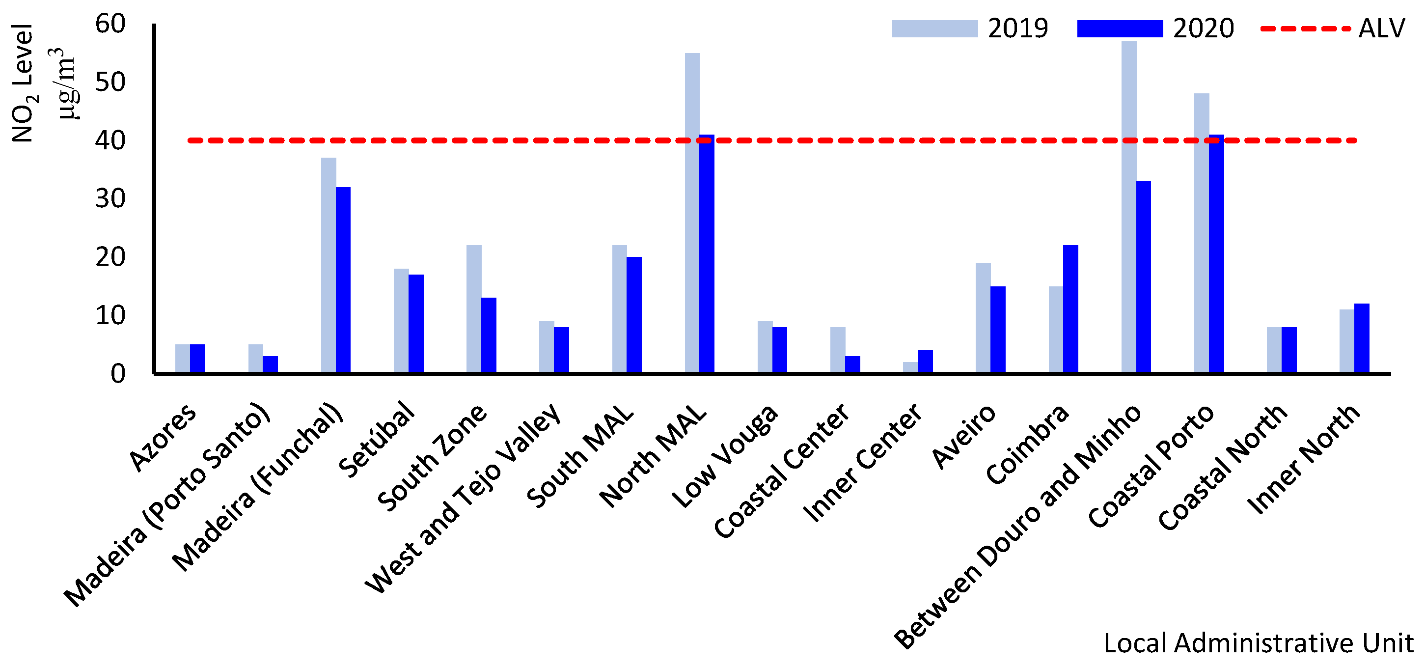
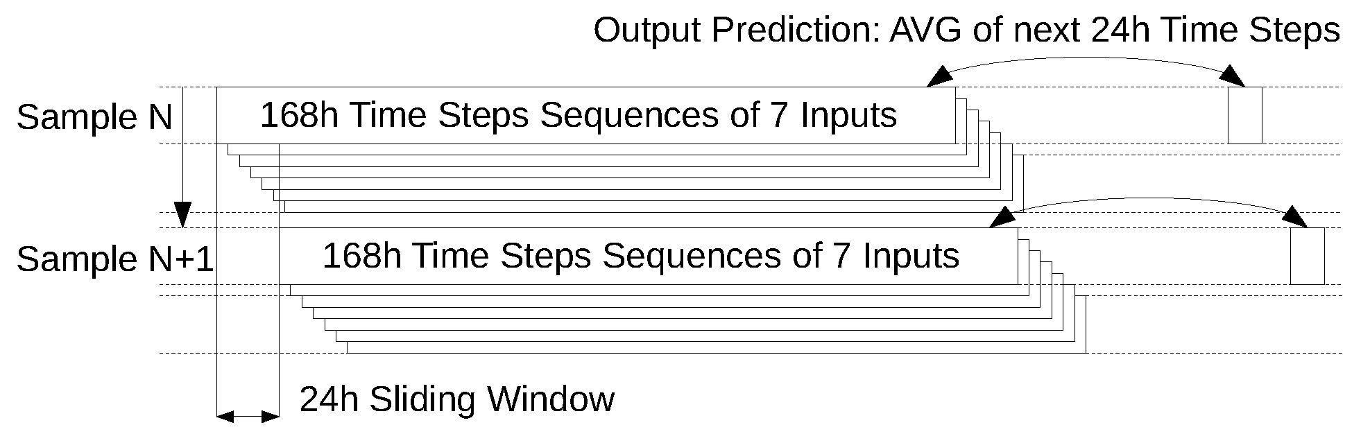
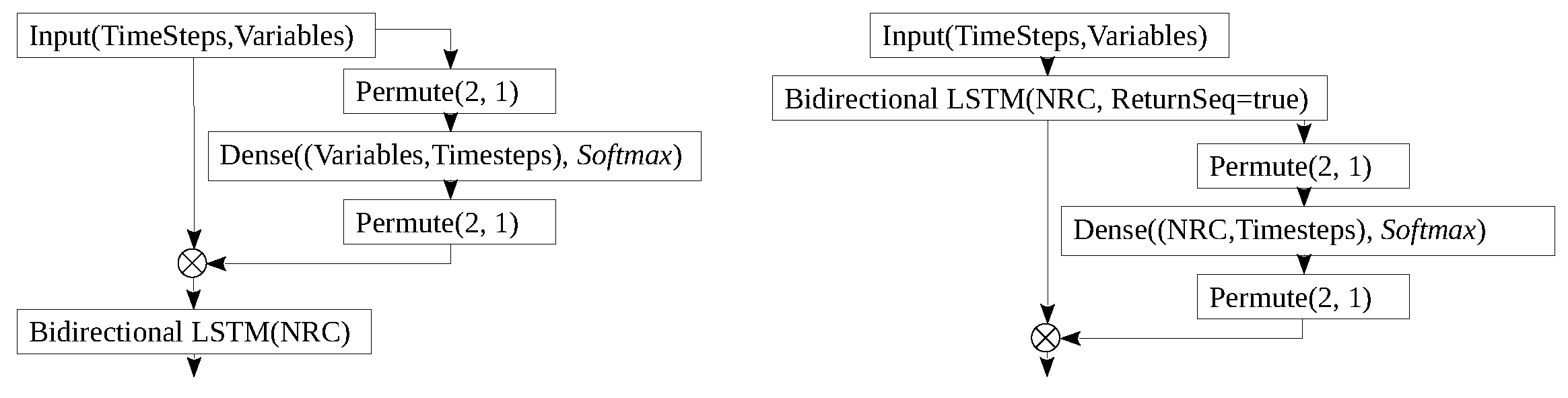
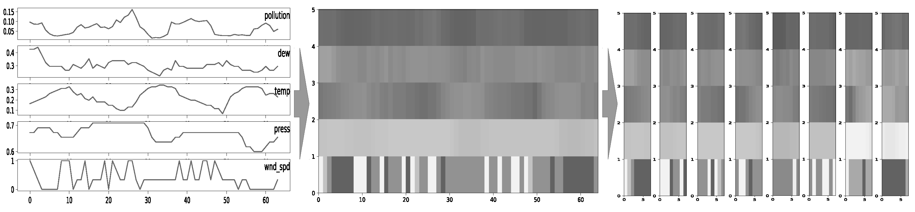
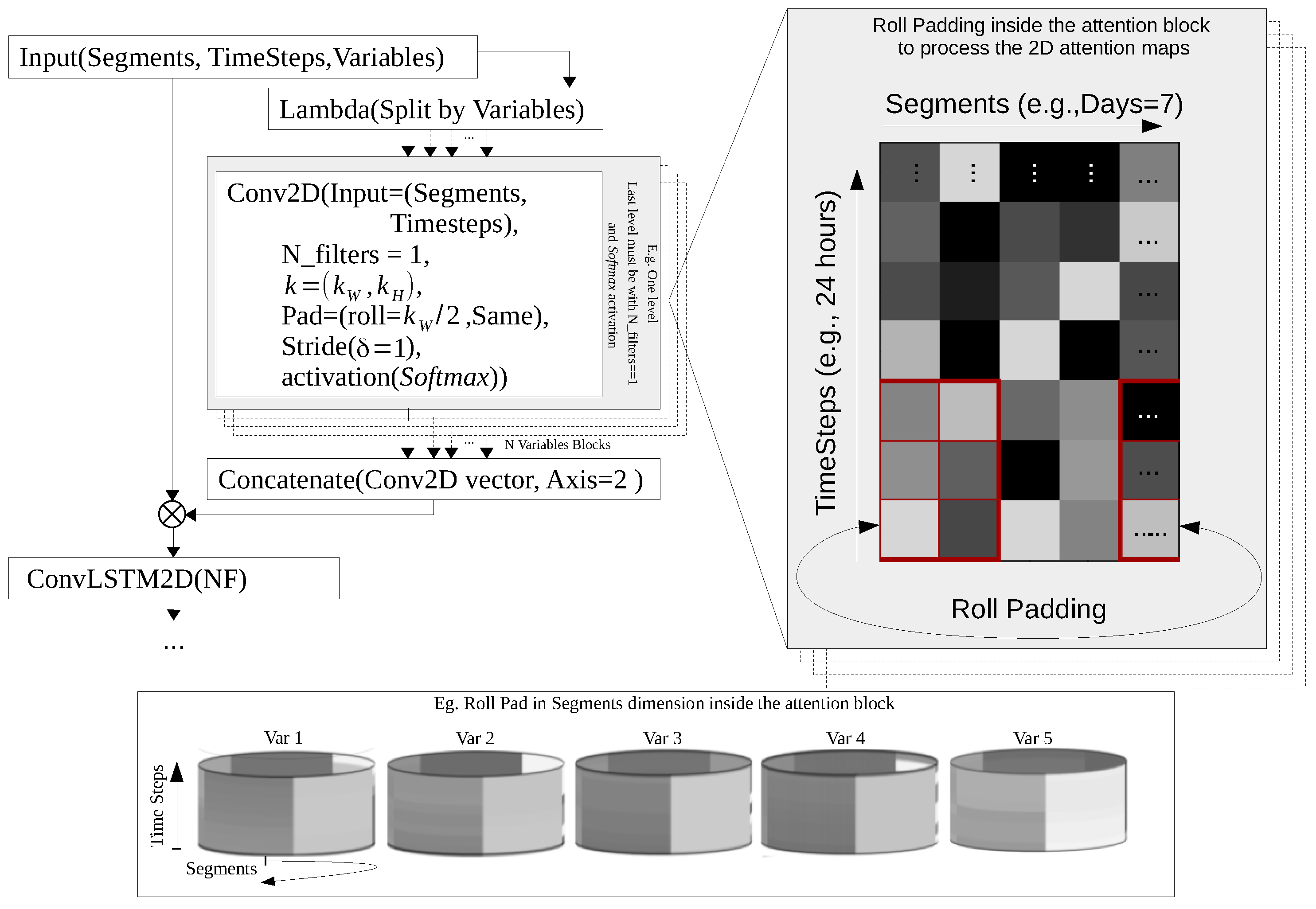
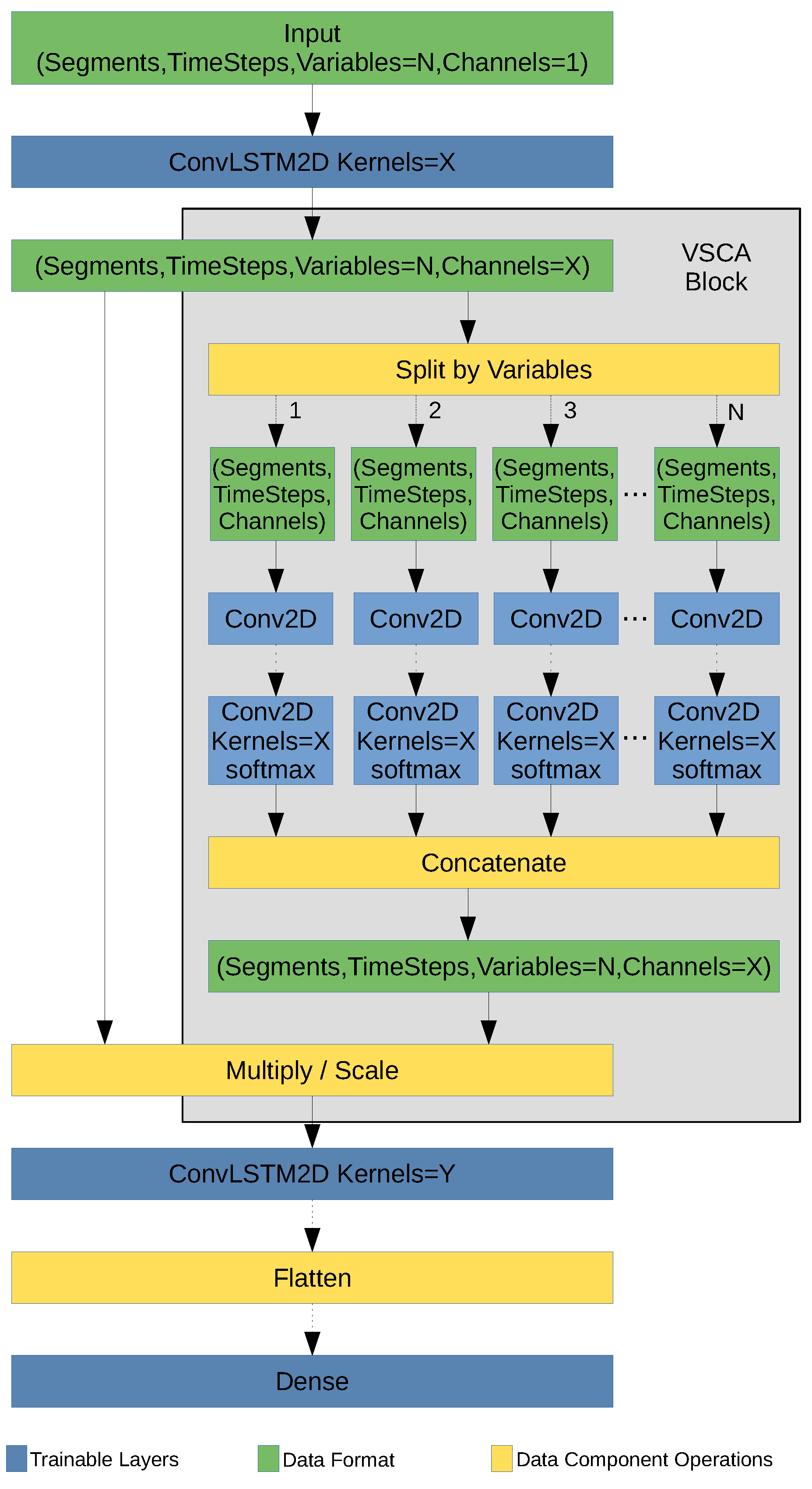
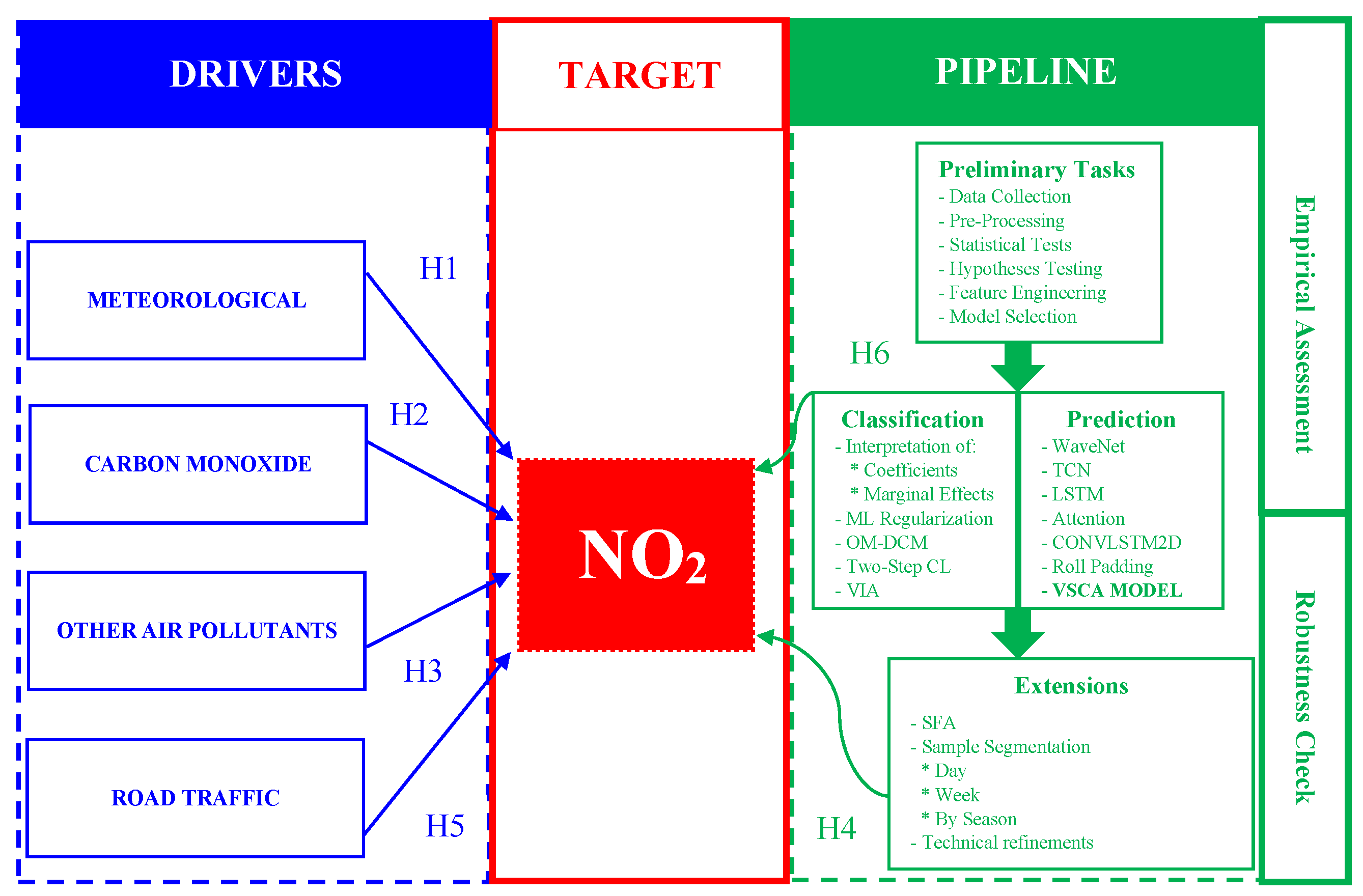
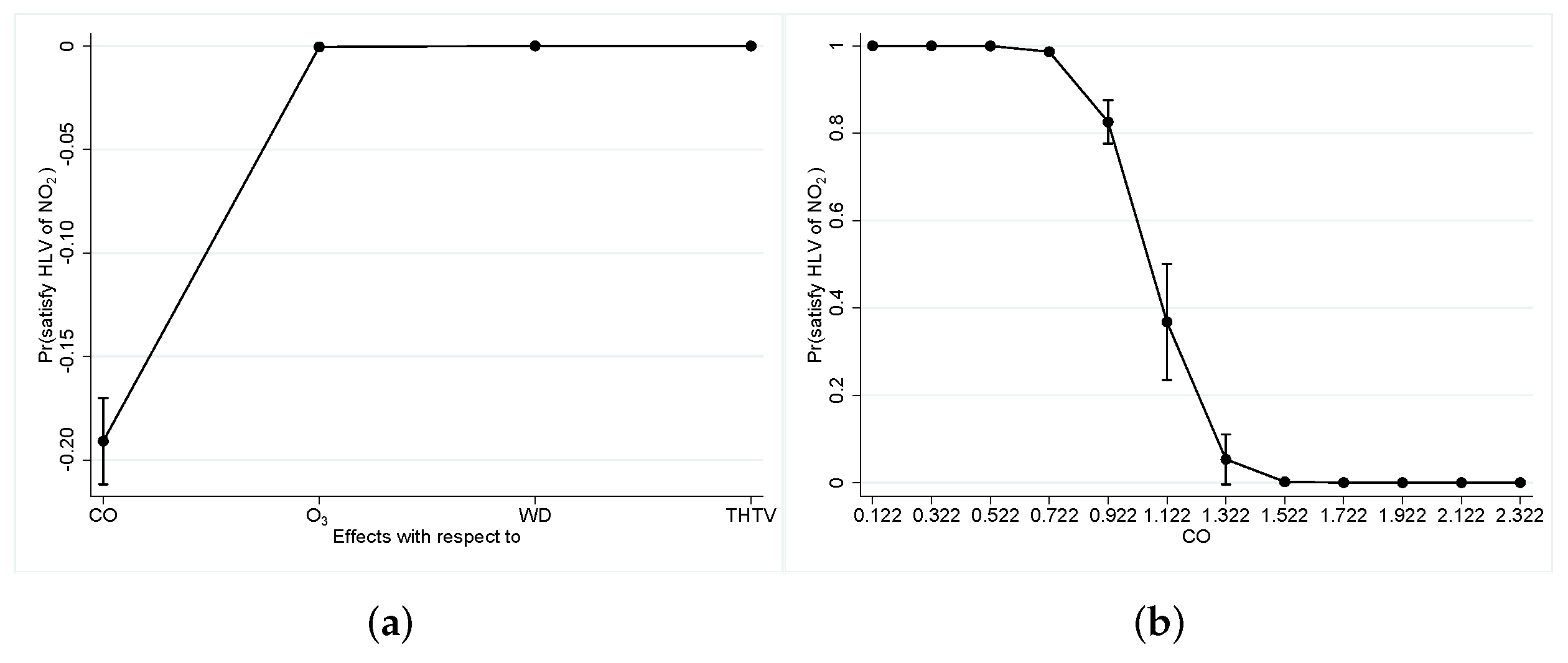
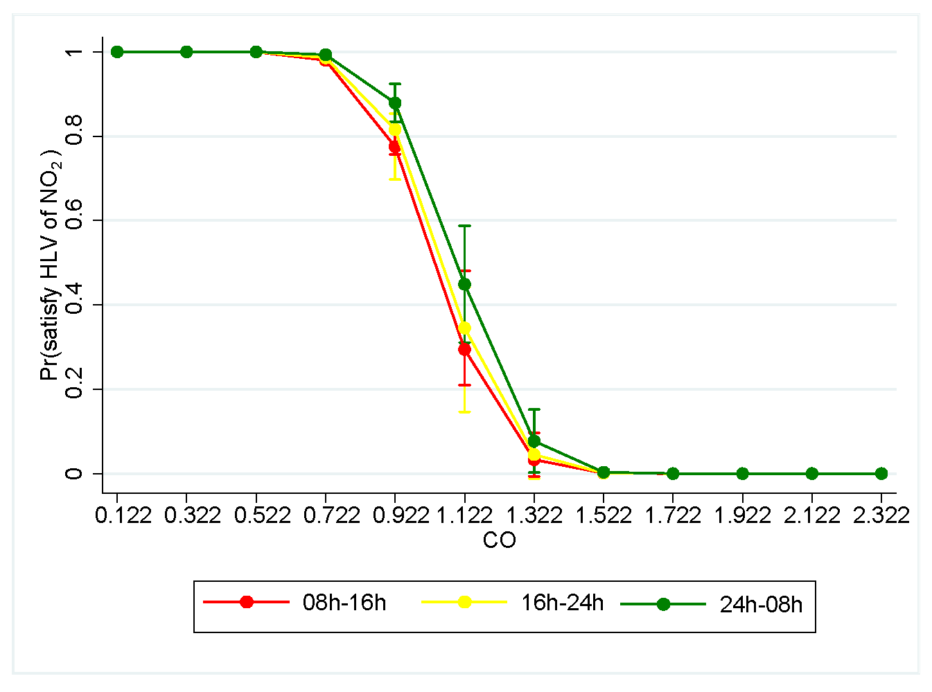
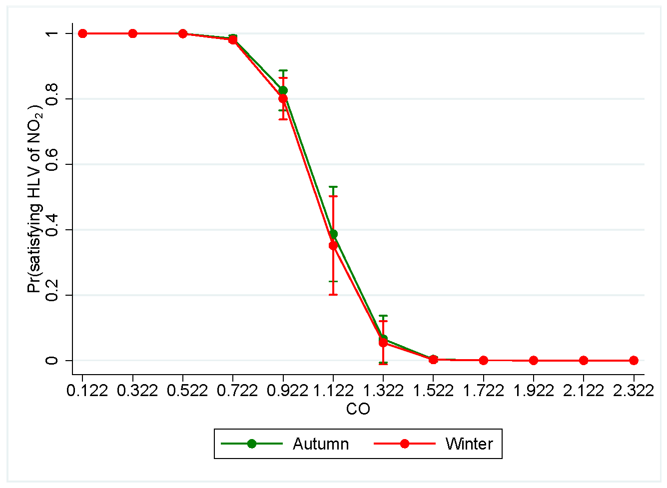
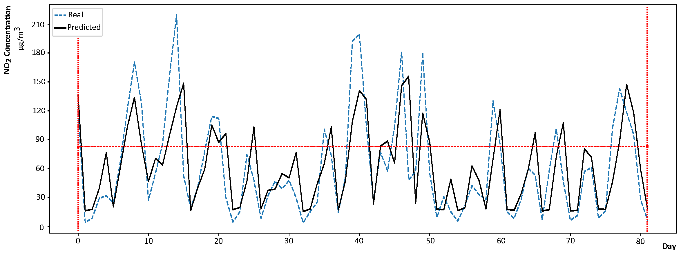
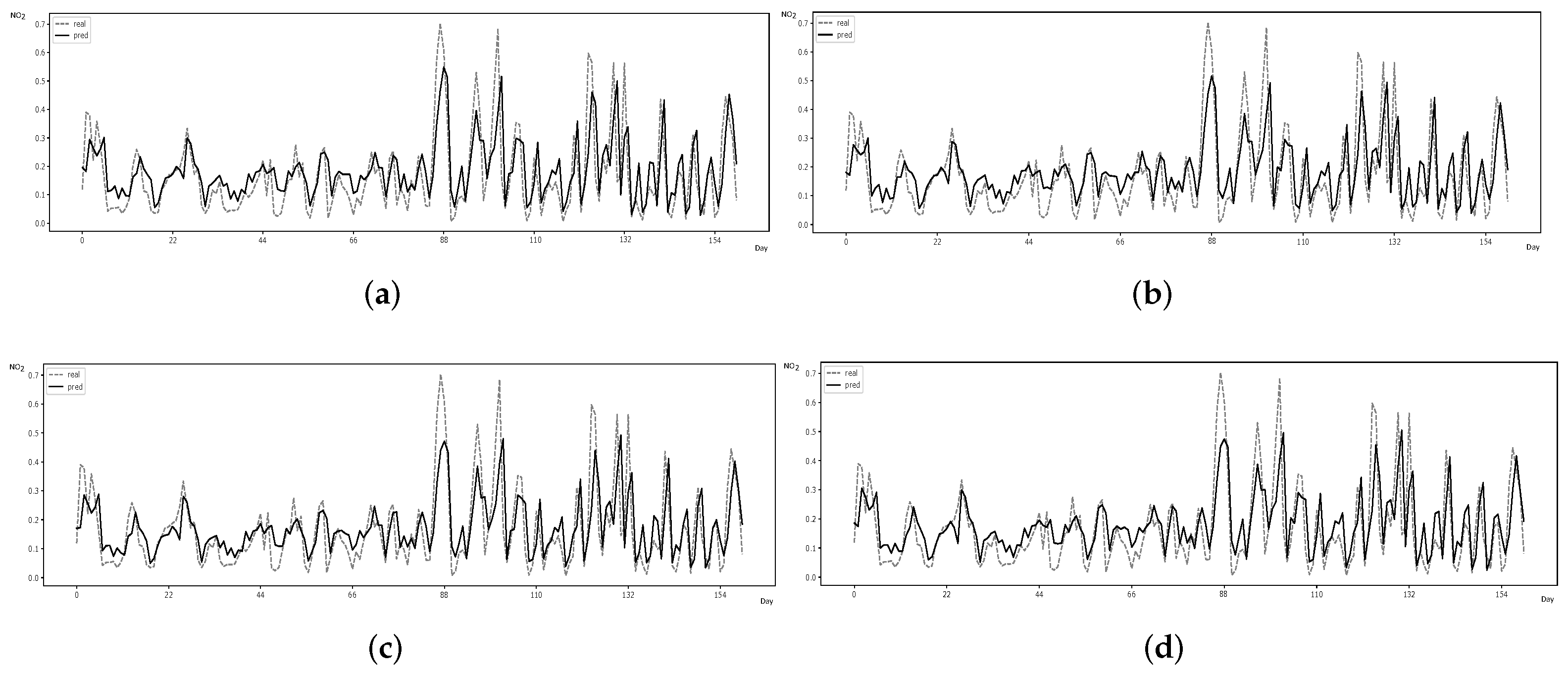
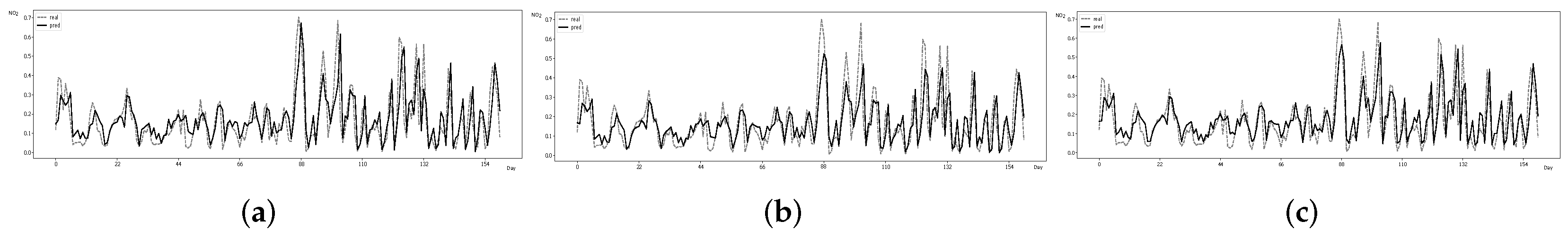
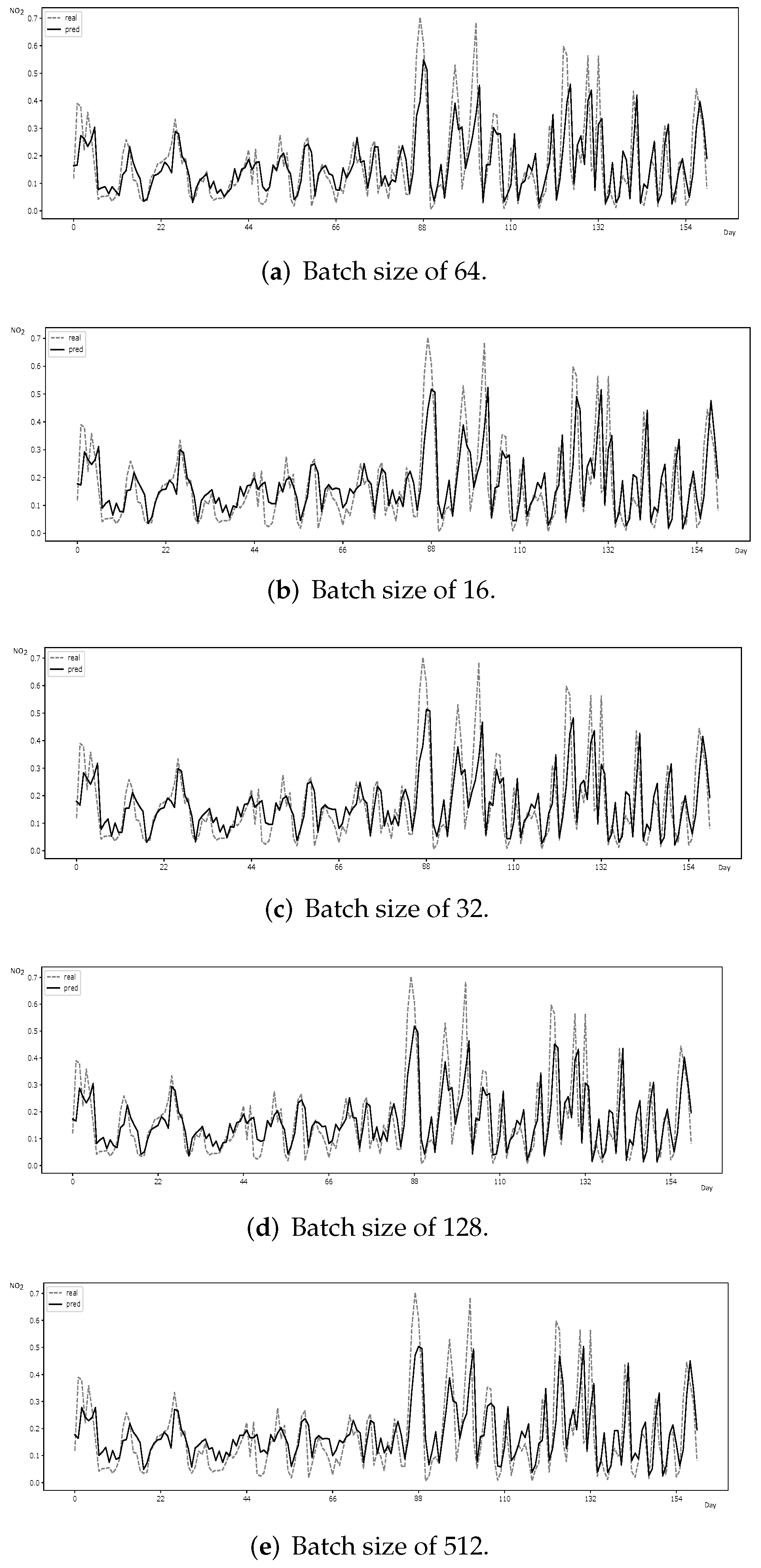
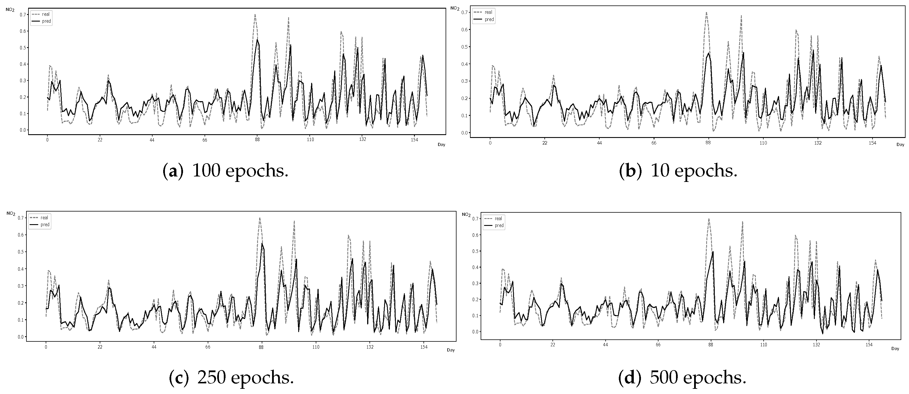
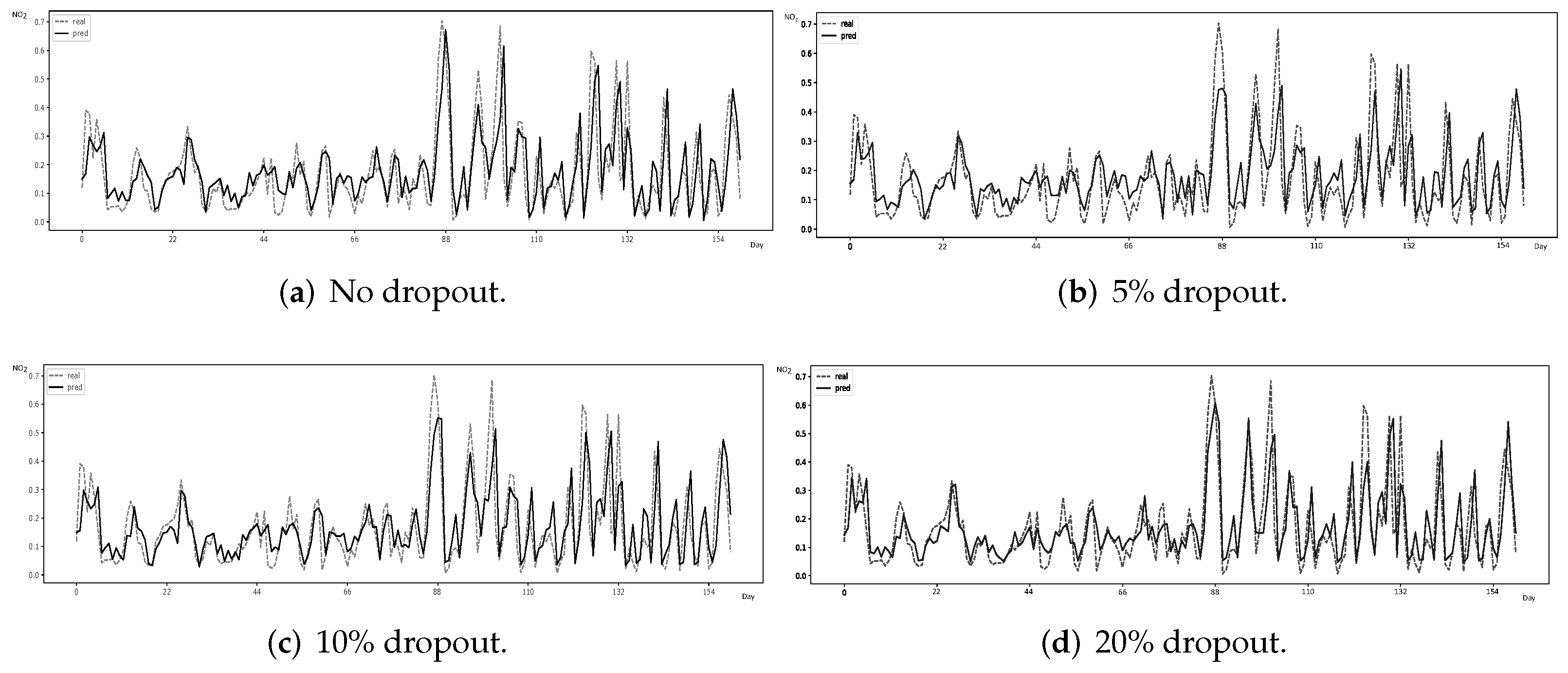
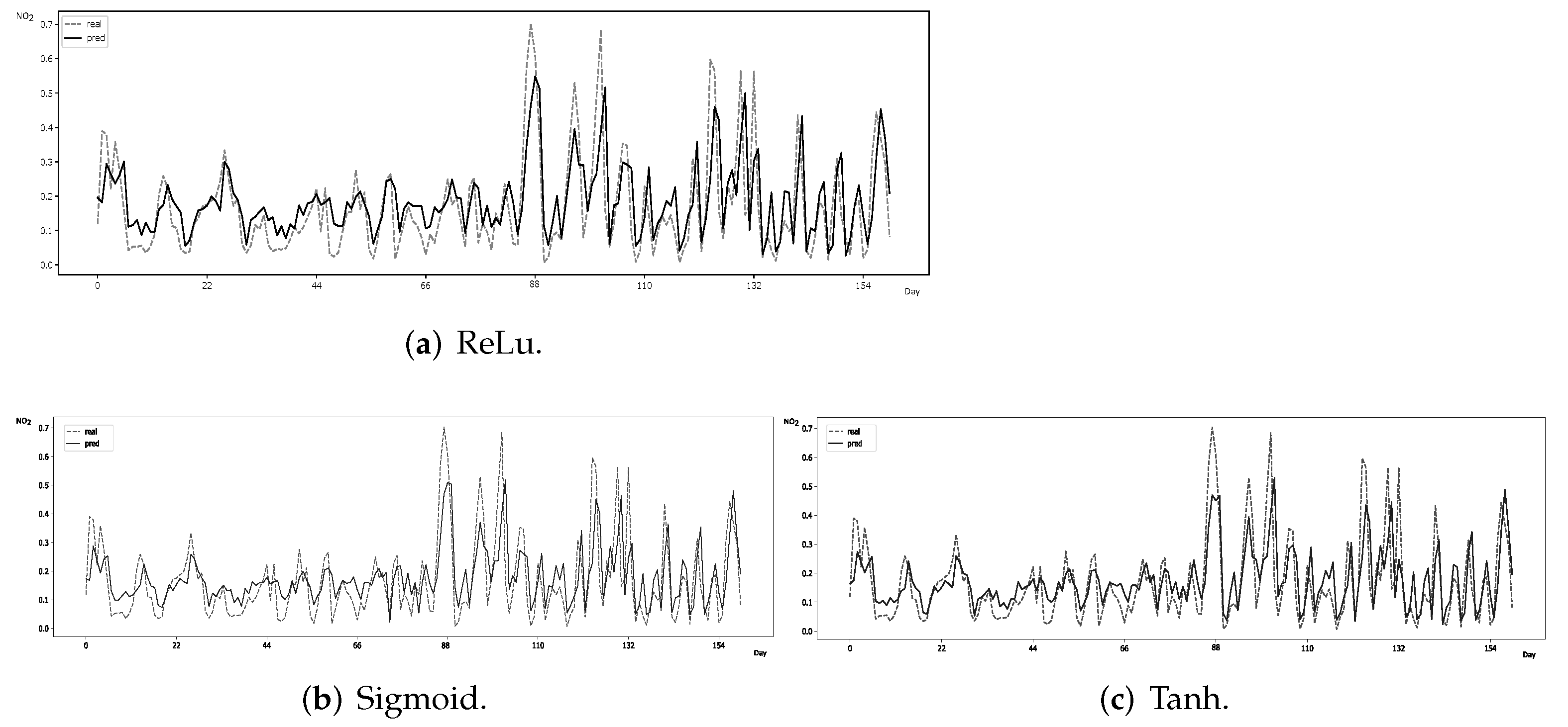
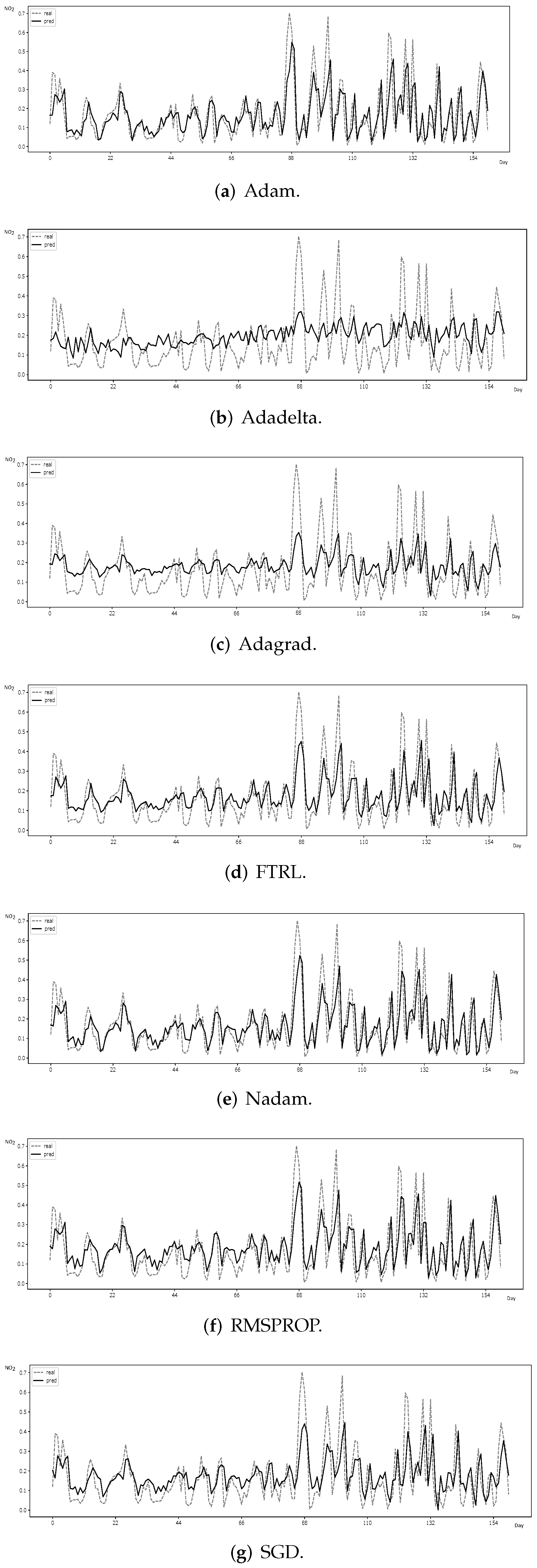
Table 1.
Summary statistics.
| Dimension | Variable | Description | Unit | Mean | Std. Dev. | Min | Max |
|---|---|---|---|---|---|---|---|
| Target | NO | Nitrogen dioxide for prediction | g/m | 82.728 | 64.421 | 0 | 341 |
| NO | Nitrogen dioxide above/below the HLV for classification | Dummy | 0.963 | 0.189 | 0 | 1 | |
| Air quality | O | Ozone | g/m | 759.954 | 43.411 | 0 | 309 |
| PM | Particle matter with a diameter of less than 2.5 m | g/m | 7.569 | 5.732 | 0 | 105 | |
| PM | Particle matter with a diameter of less than 10 m | g/m | 20.661 | 13.591 | 2 | 251 | |
| CO | Carbon monoxide | mg/m | 0.587 | 0.151 | 0.122 | 2.379 | |
| Noise | ECSL | Equivalent continuous sound level | dB(A) | 68.508 | 3.603 | 40 | 93 |
| Road traffic | THTV | Total hourly traffic volume | Veihicles | 853.027 | 883.473 | 0 | 3087 |
| Weather | AP | Atmospheric pressure | mbar | 1005.860 | 211.626 | 972 | 1127 |
| RH | Relative humidity | % | 0.651 | 0.153 | 0.164 | 0.937 | |
| T | Temperature | °C | 19.042 | 5.004 | 7.2 | 40.8 | |
| P | Precipitation | mm | 0.003 | 0.046 | 0 | 2.900 | |
| WI | Wind intensity | km/h | 11.885 | 6.207 | 0.400 | 55.900 | |
| WD | Wind direction | ° | 213.352 | 127.323 | 0 | 359.900 | |
| UVI | Ultraviolet index | I | 0.731 | 1.729 | 0 | 10 |
Notes: time-step resolution in hours. Total number of observations corresponds to n = 7824. ‘I’ stands for index and ‘o’ stands for degrees. Target, air quality, noise, road traffic, AP, RH and T input variables are collected from the sensor located at Avenida da Républica [Degrees, minutes and seconds (DMS) coordinates: 38°4409.4 N 9°0844.4 W]. P comes from the sensor located at Praça de Espanha (DMS coordinates: 38°4418.5 N 9°0932.3 W), whereas WI and WD stem from the sensor located in Chelas—Rua Dr. José Espirito Santo (DMS coordinates: 38°4509.0 N 9°0620.5 W). UVI is collected from the sensor installed in Olivais Sul—Quinta Pedagógica (DMS coordinates: 38°4548.1 N 9°0642.4 W).
Table 2.
Correlation matrix and variable inflation factor.
| NO | O | PM | PM | CO | ECSL | THTV | AP | RH | T | P | WI | WD | UVI | VIF | |
|---|---|---|---|---|---|---|---|---|---|---|---|---|---|---|---|
| NO | 1 | ||||||||||||||
| O | 0.503 *** | 1 | 1.14 | ||||||||||||
| PM | 0.347 *** | 0.109 *** | 1 | 331.30 | |||||||||||
| PM | 0.347 *** | 0.109 *** | 0.999 *** | 1 | 331.08 | ||||||||||
| CO | 0.504 *** | 0.145 *** | 0.460 *** | 0.459 *** | 1 | 1.33 | |||||||||
| ECSL | 0.047 *** | 0.032 *** | −0.013 | −0.013 | −0.021 | 1 | 1.02 | ||||||||
| THTV | −0.286 *** | −0.071 *** | −0.031 *** | −0.031 *** | −0.112 *** | −0.053 *** | 1 | 1.06 | |||||||
| AP | 0.134 *** | 0.047 *** | 0.095 *** | 0.095 *** | 0.082 *** | −0.046 *** | 0.050 *** | 1 | 1.10 | ||||||
| RH | 0.196 *** | 0.151 *** | 0.114 *** | 0.115 *** | 0.143 *** | −0.109 *** | −0.0001 | 0.037 *** | 1 | 1.06 | |||||
| T | −0.196 *** | −0.177 *** | −0.167 *** | −0.168 *** | −0.097 *** | −0.009 | −0.020 * | −0.265 *** | −0.073 *** | 1 | 1.17 | ||||
| P | 0.043 *** | 0.008 | 0.020 * | 0.020 * | −0.001 | 0.018 | −0.033 *** | 0.034 *** | −0.012 | −0.033 *** | 1 | 1.00 | |||
| WI | −0.182 *** | −0.037 *** | −0.089 *** | −0.088 *** | −0.055 *** | 0.009 | 0.111 *** | -−0.032 *** | −0.036 *** | −0.014 | −0.004 | 1 | 1.09 | ||
| WD | −0.226 *** | −0.059 *** | −0.062 *** | −0.062 *** | −0.116 *** | −0.010 | 0.121 *** | −0.123 *** | −0.094 *** | 0.159 *** | −0.037 *** | 0.238 *** | 1 | 1.13 | |
| UVI | −0.078 *** | 0.195 *** | −0.059 *** | −0.060 *** | −0.099 *** | −0.016 | 0.101 *** | −0.070 *** | −0.016 | 0.077 *** | −0.012 | 0.115 *** | 0.026 ** | 1 | 1.10 |
Notes: *** (**) [*] denotes statistical significance at the 1% (5%) [10%] level, respectively. Inputs in red color are excluded to avoid multicollinearity concerns.
Table 3.
Preliminary statistical tests.
| Test | Null Hypothesis (H0) | Value | Decision Applied to the Prediction Exercise |
|---|---|---|---|
| 1. Normality | Normal errors’ distribution | ||
| Jarque–Bera LM | 120 *** [2] | Rej H0: absence of data normality. | |
| Doornik–Hansen LM | 4,850,000 *** [24] | Thus, use feature engineering | |
| Henze–Zirkler | 7.287 *** [1] | in the prediction exercise. | |
| 2. Skewness | Zero skewness | ||
| Mardia | 1840.521 *** [364] | Rej H0: presence of data skewness. | |
| Cameron–Trivedi | |||
| Skewness decomposition | 777.260 *** [11] | ||
| 3. Kurtosis | Zero excess kurtosis | ||
| Mardia | 2563.017 *** [1] | Rej H0. | |
| Cameron–Trivedi Skewness decomposition | 1.300 [1] | Do not rej H0. | |
| 4. Homoscedasticity | Disturbance term has a constant variance | ||
| White IM | 1542.610 *** [77] | Rej H0: presence of | |
| Breusch–Pagan | 331.470 *** [1] | heteroscedasticity. | |
| 5. White noise | Disturbance term follows a white noise | ||
| Portmanteau Q | 189,100 *** [40] | ||
| 6. Autocorrelation | No serial correlation | ||
| Durbin–Watson (12; 7824) | |||
| Durbin’s alternative | 37,343.759 *** [1] | Rej H0: evidence of | |
| Breusch–Godfrey LM | 6470.582 *** [1] | positive autocorrelation. | |
| ARCH LM | 3964.158 *** [1] | ||
| 7. Number of NO lags to add as inputs | |||
| LL: −33,048.900; LR: 14.009 *** [1]; FPE: 276.947; AIC: 8.462; HQIC: 8.465; BIC: 8.472 | |||
| 8. Stationary | Target has unit root | ||
| Augmented Dickey–Fuller | |||
| 9. Specification | Model has no omitted variables | ||
| Ramsey F(3; 7809) | 65.090 *** | ||
Notes: *** denotes statistical significance at the 1% level. Degrees of freedom are displayed in brackets. ‘ARCH’ stands for autoregressive conditional heteroscedasticity. ‘LL’ stands for log-likelihood, ‘LR’ stands for likelihood ratio, ‘FPE’ stands for final prediction error, ‘AIC’ stands for Akaike information criterion, ‘HQIC’ stands for Hannan–Quinn information criterion and ‘BIC’ stands for Bayesian information criterion.
Table 4.
Hypotheses testing for individual and joint significance of input variables.
| Test | Null Hypothesis (H0) | Value | Decision Applied to the Classification Exercise |
|---|---|---|---|
| 1. Joint significance | Nonsignificant covariates | ||
| Wald with logit (probit) applied to ECSL, AP, RH, T, P, WI and UVI | 6.360 (5.180) [7] | ||
| LR with logit (probit) applied to ECSL, AP, RH, T, P, WI and UVI | 5.020 (3.740) [7] | ||
| 2. Individual significance | Nonsignificant covariate | ||
| Wald with logit (probit) applied to ECSL | 0.000 (0.010) [1] | ||
| Wald with logit (probit) applied to AP | 2.810 * (1.130) [1] | ||
| Wald with logit (probit) applied to RH | 0.010 (0.140) [1] | ||
| Wald with logit (probit) applied to T | 0.380 (0.030) [1] | ||
| Wald with logit (probit) applied to P | 0.020 (0.020) [1] | ||
| Wald with logit (probit) applied to WI | 1.330 (1.170) [1] | ||
| Wald with logit (probit) applied to UVI | 0.210 (1.140) [1] | ||
| Wald with logit (probit) applied to O | 159.200 *** (127.540 ***) [1] | ||
| Wald with logit (probit) applied to CO | 195.960 *** (183.290 ***) [1] | ||
| Wald with logit (probit) applied to THTV | 6.170 ** (4.710 **) [1] | ||
| Wald with logit (probit) applied to WD | 20.490 *** (23.780 ***) [1] | ||
Notes: *** (**) [*] denotes statistical significance at the 1% (5%) [10%] level, respectively. Degrees of freedom (results with probit estimation) are displayed in brackets (parentheses), respectively. ‘LR’ stands for likelihood ratio. Inputs in red color should be disregarded from the classification exercise.
Table 5.
Main results of the classification analysis.
| Regression Models for the Target NO | Discrete Choice Models for the Binary Dependent Variable NO | |||||||||
|---|---|---|---|---|---|---|---|---|---|---|
| (1) | (2) | (3) | (4) | (5) | (6) | |||||
| Coefficient | Coefficient | Coefficient | Coefficient/ | Coefficient | Marginal Effect | Coefficient | Marginal Effect | |||
| Marginal Effect | Average | At the Mean | Average | At the Mean | ||||||
| Input variable | ||||||||||
| CO | ||||||||||
| O | ||||||||||
| THTV | ||||||||||
| WD | ||||||||||
| Independent term | ||||||||||
| Performance metrics | ||||||||||
| RMSE | ||||||||||
| AIC | ||||||||||
| BIC | ||||||||||
| Log-likelihood | ||||||||||
| Pseudo- | ||||||||||
| Sensitivity | ||||||||||
| Specificity | ||||||||||
| Accuracy | ||||||||||
Notes: *** (**) [*] denotes statistical significance at the 1% (5%) [10%] level, respectively. Column (1) shows OLS estimation without heteroscedasticity correction, column (2) presents OLS estimation with heteroscedasticity correction by the White’s procedure, column (3) displays Cochrane–Orcutt AR(1) regression to correct for the presence of autocorrelation, column (4) exhibits LPM estimation with heteroscedasticity correction by the White’s procedure, column (5) reveals the Logit estimation and column (6) provides results from the Probit estimation. Statistical criteria (i.e., either the lowest AIC and BIC or the highest log-likelihood value) imply that probit is the best model to fit the data being, thus, the one whose coefficients and marginal effects are subject to interpretation.
Table 6.
Outcomes considering three regularization techniques combined with Logistic LASSO.
| Technique | k-Fold Cross-Validation (Assumption: 5 Folds) | Rigorous Penalization | Information Criteria | |||||
|---|---|---|---|---|---|---|---|---|
| Criterion | LOPT ( * = 6.473) | LSE ( * = 61.756) | Either AIC, BIC or EBIC ( * = 8.994) | |||||
| Model | Logistic LASSO | Post-Estimation Logit | Logistic LASSO | Post-Estimation Logit | Logistic LASSO | Post-Estimation Logit | Logistic LASSO | Post-Estimation Logit |
| Input Variable | Coefficient | Coefficient | Coefficient | Coefficient | Coefficient | Coefficient | Coefficient | Coefficient |
| O | −0.027 *** | −0.030 *** | −0.015 *** | −0.029 *** | −0.008 *** | −0.028 *** | −0.026 *** | −0.030 *** |
| CO | −12.885 *** | −13.428 *** | −10.411 *** | −13.486 *** | −9.223 *** | −13.641 *** | −12.706 *** | −13.428 *** |
| AP | −0.013 *** | −0.021 *** | −0.009 *** | −0.021 *** | ||||
| WI | 0.013 *** | 0.022 *** | 0.01 *** | 0.022 *** | ||||
| WD | 0.003 *** | 0.004 *** | 0.0005 *** | 0.004 *** | 0.003 *** | 0.004 *** | ||
| THTV | 0.0002 *** | 0.0003 *** | 0.0002 *** | 0.0003 *** | ||||
| Independent term | 26.577 *** | 35.414 *** | 11.559 *** | 14.781 *** | 10.219 *** | 15.420 *** | 22.952 *** | 35.414 *** |
| Performance metrics(after converting the classification problem into a regression problem) | ||||||||
| RMSE | 0.129 | 0.137 | 0.129 | |||||
| MAE | 0.032 | 0.041 | 0.033 | |||||
| MAPE | 0.016 | 0.020 | 0.016 | |||||
| Theil’s U | 0.851 | 0.851 | 0.844 | |||||
| 67.394 *** | 66.897 *** | 67.321 *** | ||||||
Notes: *** denotes statistical significance at the 1% level. ‘LOPT’ describes the penalty level that minimizes the cross-entropy loss measure, while ‘LSE’ corresponds to the largest penalty level for which the mean square prediction error is within standard errors of the minimum loss. The Wilcoxon signed-rank test checks the null hypothesis that the median of samples containing actual and predicted values of the target are equal.
Table 7.
Second-step outcomes with continual learning approach.
| Method | Probit | Logit | ||||||
|---|---|---|---|---|---|---|---|---|
| Coefficient | Coefficient | Coefficient | Marginal Effect | Coefficient | Marginal Effect | |||
| Input Variable | Average | At the Mean | Average | At the Mean | ||||
| O | ||||||||
| CO | ||||||||
| WD | ||||||||
| THTV | ||||||||
| Independent term | ||||||||
| Performance metrics | ||||||||
| 0.969 | 0.967 | |||||||
| RMSE | 0.033 | 0.033 | ||||||
| AIC | 896.743 | 909.199 | ||||||
| BIC | 931.567 | 944.024 | ||||||
| Log pseudolikelihood | −443.371 | −449.599 | ||||||
Notes: *** (**) denotes statistical significance at the 1% (5%) level, respectively. OLS estimation with correction of heteroscedasticity serves to confirm that the linear predicted probability of the target estimated by RF in the first-step, rather than its quadratic version, should be the one used as explained variable in the second-step of CL.
Table 8.
Outcomes with ordered multinomial discrete choice models.
| Type of Ordered Multinomial Discrete Choice Model | Probit | ||||||
|---|---|---|---|---|---|---|---|
| Input Variable | Coefficient | Marginal Effect | |||||
| Average | At the Mean | ||||||
| CO | |||||||
| O | |||||||
| WD | |||||||
| THTV | |||||||
| Cut | |||||||
| Cut | |||||||
| Performance metrics | |||||||
| AIC | 4041.474 | ||||||
| BIC | 4083.263 | ||||||
| Log pseudolikelihood | −2014.737 | ||||||
| CO | |||||||
| O | |||||||
| WD | |||||||
| THTV | |||||||
| Cut | |||||||
| Cut | |||||||
| Performance metrics | |||||||
| AIC | 4040.452 | ||||||
| BIC | 4082.242 | ||||||
| Log pseudolikelihood | −2014.226 | ||||||
Notes: *** (*) denotes statistical significance at the 1% (10%) level, respectively.
Table 9.
Outcomes of time-variant models for stochastic frontier analysis.
| Model | Tfe SFA | Tre SFA | MLrei SFA | ILSfe SFA | MLred SFA | LSDVfe SFA |
|---|---|---|---|---|---|---|
| Input Variable | Coefficient | Coefficient | Coefficient | Coefficient | Coefficient | Coefficient |
| O | ||||||
| CO | ||||||
| WD | ||||||
| THTV | ||||||
| Independent term | ||||||
| Performance metrics | ||||||
| Log likelihood | −40,854.017 | −40,854.017 | −40,840.225 | −40,890.490 | −40,890.490 | −40,890.490 |
Notes: *** denotes statistical significance at the 1% level, respectively. The regression includes robust standard errors, which adjust for within-cluster correlation. THTV is the explanatory variable specified for the inefficiency variance function. ‘Tfe SFA’ stands for true fixed effects SFA model, whereas ‘Tre SFA’ stands for true random effects SFA model [37]. ‘MLrei SFA’ stands for maximum likelihood random effects time-varying inefficiency effects model [38]. ‘ILSfe SFA’ stands for iterative least squares time-varying fixed effects model [39]. ‘MLred SFA’ stands for maximum likelihood random effects time-varying efficiency decay model [40]. ‘LSDVfe SFA’ stands for modified least squares dummy variable time-varying fixed effects model [41].
Table 10.
Forecasting errors in the test set with normalized output values.
| DLNN Model | RMSE | MSE | MAE |
|---|---|---|---|
| WaveNet | 0.10169 | 0.01034 | 0.06713 |
| TCN | 0.10383 | 0.01078 | 0.06753 |
| LSTM | 0.09859 | 0.00972 | 0.06691 |
| LSTM with Standard Attention Mechanism | 0.09550 | 0.00912 | 0.06586 |
| LSTM with Conv1D Attention | 0.09192 | 0.00845 | 0.06499 |
| ConvLSTM2D | 0.09889 | 0.00978 | 0.06597 |
| ConvLSTM2D with Conv2D Attention and roll padding (VSCA) | 0.08940 | 0.00799 | 0.06414 |
Publisher’s Note: MDPI stays neutral with regard to jurisdictional claims in published maps and institutional affiliations. |
© 2022 by the authors. Licensee MDPI, Basel, Switzerland. This article is an open access article distributed under the terms and conditions of the Creative Commons Attribution (CC BY) license (https://creativecommons.org/licenses/by/4.0/).
Share and Cite
MDPI and ACS Style
Ribeiro, V.M.; Gonçalves, R. Classification and Prediction of Nitrogen Dioxide in a Portuguese Air Quality Critical Zone. Atmosphere 2022, 13, 1672. https://doi.org/10.3390/atmos13101672
AMA Style
Ribeiro VM, Gonçalves R. Classification and Prediction of Nitrogen Dioxide in a Portuguese Air Quality Critical Zone. Atmosphere. 2022; 13(10):1672. https://doi.org/10.3390/atmos13101672
Chicago/Turabian StyleRibeiro, Vitor Miguel, and Rui Gonçalves. 2022. "Classification and Prediction of Nitrogen Dioxide in a Portuguese Air Quality Critical Zone" Atmosphere 13, no. 10: 1672. https://doi.org/10.3390/atmos13101672
Note that from the first issue of 2016, this journal uses article numbers instead of page numbers. See further details here.