
Monitoring of Expansive Clays over Drought-Rewetting Cycles Using Satellite Remote Sensing
by
 , ,
, ,
André Burnol
1,* ,
,
Michael Foumelis
1,2,*,
Sébastien Gourdier
1,
Jacques Deparis
1 and
Daniel Raucoules
1 1
BRGM, Risks and Risk Prevention Division (DRP), 45060 Orléans, France
2
Department of Physical and Environmental Geography, Aristotle University of Thessaloniki (AUTh), 54124 Thessaloniki, Greece
*
Authors to whom correspondence should be addressed.
Atmosphere 2021, 12(10), 1262; https://doi.org/10.3390/atmos12101262
Submission received: 21 July 2021
/
Revised: 23 September 2021
/
Accepted: 24 September 2021
/
Published: 28 September 2021
(This article belongs to the Special Issue Drought Risk Management in Reflect Changing of Meteorological Conditions)
Abstract
:New capabilities for measuring and monitoring are needed to prevent the shrink-swell risk caused by drought-rewetting cycles. A clayey soil in the Loire Valley at Chaingy (France) has been instrumented with two extensometers and several soil moisture sensors. Here we show by direct comparison between remote and in situ data that the vertical ground displacements due to clay expansion are well-captured by the Multi-Temporal Synthetic Aperture Radar Interferometry (MT-InSAR) technique. In addition to the one-year period, two sub-annual periods that reflect both average ground shrinking and swelling timeframes are unraveled by a wavelet-based analysis. Moreover, the relative phase difference between the vertical displacement and surface soil moisture show local variations that are interpreted in terms of depth and thickness of the clay layer, as visualized by an electrical resistivity tomography. With regard to future works, a similar treatment relying fully on remote sensing observations may be scaled up to map larger areas in order to better assess the shrink-swell risk.
1. Introduction
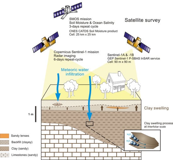
Among the various natural risks in France, the risk due to shrinking and swelling of subsurface clays is the second most important cause of financial compensation from insurance companies behind the flooding risk. In 2010, a first shrink/swell hazard map of metropolitan France, based on 1:50,000 geological maps, geotechnical data and spatial distribution of building damages has been published by the French Geological Survey (BRGM). So far, in situ monitoring of soil moisture and ground movements and ex situ clay characterization are traditionally used to assess this risk (e.g., the Mormoiron site with a Mediterranean climate [1] or at the Pessac site with an oceanic climate [2]). Since 2016, a new site characterized by a high shrink/swell hazard, level and located at Chaingy (France) has been instrumented by BRGM.
Standard ground displacement monitoring techniques (e.g., extensometers and GNSS) provide information on a very limited number of points within an area. Allowing a higher density of measurement points, the monitoring using Multi-Temporal Synthetic Aperture Radar Interferometry (MT-InSAR) techniques has been intensively developed in the last decades to track land subsidence or uplift related to groundwater extraction or recharge of aquifers around large cities [3,4,5]. Conversely, the monitoring of expansive clays based on InSAR has been the subject of very few studies until now [6,7,8]. The major limiting factor is the non-availability of relatively high-temporal resolution remote sensing datasets. There is indeed the requirement for fine temporal sampling due to the non-linear behavior of the shrink/swell cycles [9]. The launch by the European Space Agency (ESA) of the Copernicus Sentinel-1A/1B satellites enables the systematic data provision, with a 6-day repeat cycle at the equator.
The aim of this article is to present an investigation of the shrink/swell behavior of a clay soil in relation to drought-rewetting cycles using both in situ and satellite remote sensing monitoring techniques over an instrumented site. The ground displacement measured by InSAR is compared to the in situ measurements in the studied zone during a three-year period. We will analyze how accurate Sentinel-1 data can measure the ground displacement due to the shrink/swell process, when the Parallel Small Baseline Subset (P-SBAS) technique is applied, and how well P-SBAS results and precise extensometers agree in validation for our study area. Our hypothesis is that the vertical displacement captured by the P-SBAS technique using a 90 m by 90 m cell is an average vertical displacement in that cell. Moreover, we show the time lag between the in-ground soil moistures at 1.2 m depth and the surface soil moisture acquired by the SMOS satellite. Finally, we propose for a first time a methodology for evaluating the depth and the thickness of subsurface clay layers relying fully on remote sensing observations, namely the use of the relative phase difference between Sentinel-1 InSAR displacement and SMOS surface soil moisture time series. In order to further validate this new approach, we deployed an electric tomography survey providing insights on the subsurface structure.
2. Materials and Methods
2.1. Studied Area
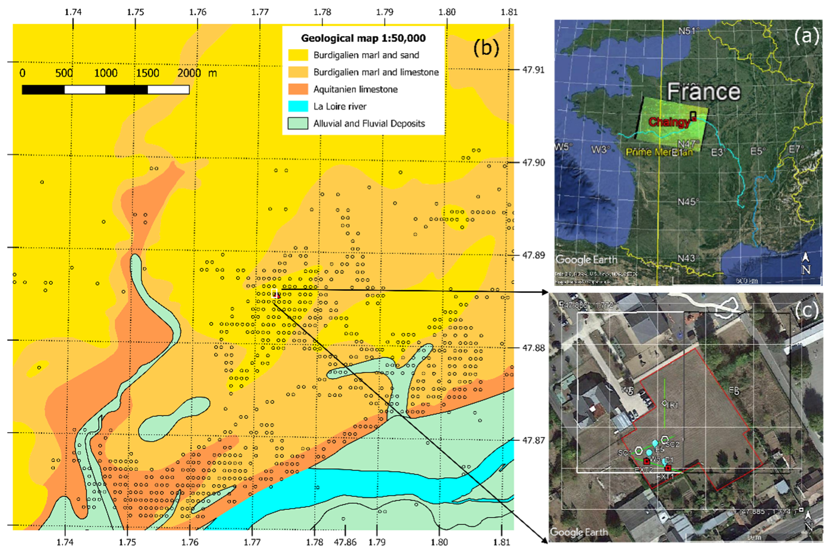
Our investigation site, an urban area located at Chaingy (France) with a semi-oceanic (i.e., slightly continental) climate, is characterized by a high level of shrink/swell hazard (Figure 1). Since 2016, two in situ extensometers (EXT1 and EXT2), spaced about 12 m apart, and a battery of soil moisture sensors at 1.2 m depth are deployed (Figure 1).
2.2. Synthetic Aperture Radar (SAR) Data and Interferometic Processing
Copernicus Sentinel-1 SAR data was utilized for the investigation of induced ground displacements in the vicinity of the extensometers EXT1 and EXT2 (see Table 1). Interferometric SAR (InSAR) processing was performed on the Geohazards Exploitation Platform (GEP) (https://geohazards-tep.eu, accessed on 23 September 2021). GEP is a platform originated by ESA as part of the Thematic Exploitation Platforms (TEP) initiative, aiming to support the exploitation of Earth Observation (EO) satellites to assess geohazards and their impact [10].
For the InSAR processing the Parallel Small Baseline Subset (P-SBAS) algorithm [11,12,13], as implemented on the GEP, was exploited. P-SBAS method is based on the processing of temporal series of co-registered SAR images acquired over the same target area for the generation of Line-of-Sight (LoS) ground displacement time series and average velocity maps. The technique allows for the extraction of both linear and non-linear motion components without a priori assumption on the displacement model. The service is provided at 90 m spacing distributed on a regular grid covering the user defined area of interest.
Between September 2016 and December 2019, the entire Sentinel-1A/1B archive data from both ascending and descending orbit geometries, 183 and 178 scenes, respectively, were processed. Supposing a 1D vertical displacement, the LOS motions are projected to vertical, whereas combination of different viewing geometries provide us the actual vertical motion component (the equation below was adapted from Hanssen (2001) [14]):
VERT is the vertical displacement, LOS the motion in the Line-Of-Sight direction, θ the incidence angle, and the subscript ASC and DES for the ascending (θASC = 34.4°) and descending (θDES = 42.8°) tracks, respectively.
2.3. SMOS Level 3 Surface Soil Moisture (SSM) Products
SMOS satellite was successfully launched on 2 November 2009 by ESA. We use here the term Surface Soil moisture (SSM) to refer to the volumetric soil moisture in the first few centimeters (0–5 cm) of the soil. L-band radiometry is achieved resulting in a ground resolution of 50 km. SMOS Level 0 (L0) to Level 2 (L2) data products are designed by ESA for scientific and operational use. The products are divided in half orbits, from pole to pole, ascending or descending, spanning about 50 min of acquisition 3. Level 3 products are geophysical variables with improved characteristics through temporal resampling or processing. In order to prevent any inconsistency resulting from interpolation over highly heterogeneous surfaces, no spatial averaging is operated in the algorithms [15,16,17]. It must also be noted that ascending and descending overpasses are bound to show different values of the retrieved parameters that may not be always comparable, and they are, thus, retrieved separately. The performance of each satellite SSM product depends on many factors such as, but not limited to, soil type, climate, presence of noise (Radio Frequency Interference), and land cover. It is therefore difficult to predict the performance of SSM products over a region, without performing a quality assessment using in situ measurements. The SMOS Level 3 SSM products were accessed through the CATDS Data Processing Center [16] (https://www.catds.fr, accessed on 23 September 2021). The data are presented over the Equal-Area Scalable Earth (EASE grid 2) [18] with a sampling of about 25 km × 25 km and the studied area is included in one grid cell (Figure 1). We used these 3-day aggregated SMOS-CATDS SSM products for ascending and descending overpasses between September 2016 and December 2019 for each Sentinel-1 acquisition (6 day-repeat cycle).
2.4. Signal Processing Using Fourier Analysis
Fourier analysis is well suited for the quantification of constant periodic components in time series. To perform filtering of satellite and in situ signals, time series of measurements are smoothed using a one-dimensional convolution approach with a HANNING window [19]. To carry out the spectral analysis, the filtered time series is first padded with trailing zeros to a length of 100 yr before computing the Discrete Fourier Transform (DFT) using the Fast Fourier Transform (FFT) Matlab (Matrix Laboratory, the MathWorks, Natick MA, USA) function [20]. The frequency maxima of Fourier power spectrum are therefore computed with a precision of 1/100 yr−1. The magnitude and the phase angles of complex FFT values are calculated by Matlab ABS and ANGLE operators, respectively. Whenever the jump between consecutive angles is greater than or equal to π radians, UNWRAP function shifts the angles by adding multiples of ±2π until the jump is less than π.
2.5. Signal Processing Using Wavelet Analysis
Fourier analysis does not provide any information about when the frequencies are present during the time-span covered by the time series. Conversely, the wavelet transform is especially suited to identify localized intermittent periodicities from low signal-to-noise ratio time-series [21,22]. The Morlet wavelet [23] is adapted to geophysical time series as described by [24] who developed the software provided at http://paos.colorado.edu/research/wavelets (accessed on 23 September 2021). We used the Matlab wavelet coherence toolbox as adapted by [25] and provided at http://www.glaciology.net/wavelet-coherence (accessed on 23 September 2021). The Continuous Wavelet Power Spectrum (CWT) expands time-series records into time/frequency space. The time-series input data must be equally spaced in time. Although Copernicus satellites have a regular revisit interval (6 days for Sentinel-1A/B and 3 days for SMOS), some acquisitions may be missing or excluded from processing. These missing values are linearly interpolated using a constant time interval. The other time-series data of extensometers and soil moistures sensors are down-sampled using the same time interval. Two individual CWTs can be combined by using the Cross Wavelet Transform (XWT) tool which is computed by multiplying the CWT of one time-series by the complex conjugate of the CWT of the second time-series. XWT image is the 2-D representation of the absolute value and the phase of the complex number in the time-frequency space. For many geophysical phenomena, an appropriate background spectrum is the red/Brownian noise (increasing power with decreasing frequency) [26]. This background spectrum was recently used in a wavelet analysis for land subsidence [27] and clay expansion [7]. ANGLEMEAN function calculates the mean angle found by XWT during a time period, and the associated sigma which corresponds to a standard deviation.
2.6. Clay Layer Characterization Using Electric Method
The data were collected using the IRIS Syscal Pro Plus multi-electrode imaging system with internal multiplexer. Three profiles were acquired using 96 stainless electrodes spaced every 30 cm. Length of the profile was 28.5 m. The measurement was carried out using Dipole–Dipole and Wenner configuration. Due to good coupling, no data was removed during pre-processing. Inversion will be carried out using Res2DINV software [28,29] with a L1 regulation norm. Root means square values was lower than 1% after fives iterations for the three profiles.
3. Results
3.1. Intercomparison of InSAR and In Situ Displacement Time Series
The InSAR LoS measurements are independently projected to the vertical as well as combined to calculate the actual vertical motion component, using the ascending track and descending track (VERT-ASC-DES) at the West Point (WP) (see Materials and Methods section). Qualitatively, there is a positive correlation between the vertical displacement VERT-ASC-DES at WP, as calculated by InSAR using the satellite observations and as measured by ground-based extensometers EXT1 and EXT2 (Figure 2). Quantitatively, the least squares correlation coefficient (cc) is much higher for EXT2 (cc = 0.69) than for EXT1 (cc = 0.47). The relatively low cc values are expected given the non-linearity phenomenon and the heterogeneities of the clay layer as described in Section 3.2.
During the three-year period, the ground displacement time-series may be decomposed with the addition of a linear trend component T, a seasonal component S and an irregular residual component. There is a linear trend with a shrinking of about −2.2 mm/yr at EXT1, while the measured motion at EXT2 is merely a cyclic component with a negligible shrinking of about −0.3 mm/yr (Figure 2). During the same period, the linear trend measured by Sentinel-1A/B lies within in situ rates at EXT1 and EXT2, with a global shrinking of about −0.55 mm/yr. Concerning the cyclic part, the expansion is up to three times higher at EXT2 than at EXT1, with average swelling of 9.4 ± 2.0 mm and 3.1 ± 1.0 mm, respectively (Figure 2). Over the same period, the swelling magnitude measured by VERT-ASC-DES is 4.5 ± 0.5 mm.
3.2. Electrical Tomography Survey
Electrical resistive tomography has been carried out in order to image the lithology stratification and the heterogeneity of the clay layer (i.e., depth, thickness, and fraction of clay) (see Materials and Methods section). Along three 28.5 m long profiles in the WP cell (Figure 1), the resistivity values range from 8 to 100 Ω.m and a three-layer stratified subsurface is highlighted (Figure 3 and Figure 4).
We used two drill cores along the SC1-SC2 profile to define the clay subsurface material by the resistivity value [30] (Figure 4). A first layer above the depth of 0.59 m ± 0.22 m corresponds to topsoil and backfill with some clay lenses (Figure 3 and Figure 4). A second layer with a mean thickness of 1.5 m ± 0.42 m corresponds to the clay material with a resistivity lower than 17 Ω.m ± 1 Ω.m. Below 2.09 m ± 0.42 m, a third layer corresponds to sandy limestones with a resistivity gradient due to the weathering process.
Along the EXT1-EXT2 resistivity profile (Figure 3), the mean depth and thickness of the clay material layer is 0.46 m ± 0.05 m (min-max, 0.34–0.55) and 1.97 m ± 0.18 m (min-max, 1.70–2.39), respectively. The mean depth of the carbonate layer is 2.43 m ± 0.16 m (min-max, 2.15–2.73). The depth (approximately at 0.5 m) and thickness (about 2.3 m) of the clay layer at EXT1 and EXT2 are very similar (Figure 3). However, the resistivity of the clay layer at EXT2 is much lower compared to EXT1, indicating that the clay fraction is much higher beneath EXT2 [20]. That is also consistent with the expansion difference between the extensometers showing a much higher swelling magnitude at EXT2.
Along the three profiles, the mean depth and thickness of the clay material layer in the West Point (WP) cell is 0.59 m ± 0.22 m and 1.5 m ± 0.42 m.
3.3. Intercomparison of In Situ Soil Moistures and SMOS Satellite Surface Soil Moistures
We investigated here the soil moisture variations acquired by E1 sensor (near EXT1) and W5 (near EXT2) that are both located at the same 1.2 m depth inside the clay layer (Figure 3). The temporal variations of E1 and W5 are strongly correlated (cc = 0.73) during the three-year period (Figure 5). For the seasonal one-year period, there is a slight leading of E1 moisture relative to W5 (about 0.75 months) as calculated by the Cross Wavelet Transform (XWT) (see Materials and Methods Section 2.5). Indeed, the infiltration time of the meteoric water inside the clay layer at 1.2 m depth is lower in the E1 case, since the clay fraction of low permeability is shallower at EXT1 compared to EXT2 (Figure 3).
We use here the term Surface Soil Moisture (SSM) to refer to the volumetric soil moisture in the first few centimeters (0–5 cm) of the soil. We investigated also the SSM acquired by the ascending (SSM-ASC) and descending (SSM-DES) orbits of the SMOS satellite, showing rather positive correlation (cc = 0.48). For the one-year period, SSM-ASC and SSM-DES are both in-phase and there is a slight leading of SSM-ASC relative to SSM-DES for the 5-month period (about 0.9 months). Hence, the SSM-ASC dataset was considered more appropriate for calculating the phase differences to other time series in the discussion. For the one-year period, the phase lead of the surface soil moisture SSM-ASC relative to the in-ground soil moistures E1 and W5 calculated by XWT is about 0.16 yr and 0.22 yr, respectively.
4. Discussion
4.1. Intercomparison of InSAR and In Situ Displacement Time Series
Displacements measured by InSAR are in the direction of the Line-of-Sight (LoS) of the satellite, while displacements measured by extensometers depict motion in the vertical direction. However, the combination of ascending and descending InSAR measurements for the calculation of the actual vertical motion component (VERT-ASC-DESC) allows the direct inter-comparison of satellite and in situ observations.
When exposed to moisture, the magnitude of the vertical expansion of soils will depend on the amount of expansive clay minerals in the subsurface. In addition to the vertical displacement, the subsurface heterogeneities (i.e., clay depth and thickness and percentage of sand) may introduce spatial variability to the observed ground displacements. The above-mentioned factors need to be considered when examining the consistency of our measurements. In our case, the vertical displacements VERT-ASC-DESC from remote sensing are within the motion values of both extensometers, not only for linear displacement rates but also in terms of observed seasonality (see Section 3.1). This result is in agreement with the assumption that the effect of the spatial resolution of the remote sensing measurements (90 m by 90 m cell) represents an average of the vertical displacements within that resolution cell.
4.2. Shrinking and Swelling Periods Using Fourier Power Spectra and Continuous Wavelet Transform
We use first the Fourier spectra of vertical displacements to calculate the main frequency components of time series of both extensometers as well as at WP and East Point (EP) cells of the P-SBAS grid. The one-year seasonal period is found in the power spectrum of the four displacement time series at EXT1, EXT2, WP, and EP (Figure 6). In the frequency band between 2 and 4 yr−1 (corresponding to a period between 0.5 and 0.25 yr), there are three other frequencies which are noted F1, F21, and F22 (order of increasing frequency) and P1, P21, and P22 periods (order of decreasing period). It should be noted that the frequency values for all displacement time series are close to the first three sub-annual components of the Fourier transform of the soil moistures E1 and W5 at 1.2 m depth (Figure 6a) and the two ascending and descending time series of the surface soil moisture (SSM-ASC and SSM-DES) as measured by SMOS (Figure 6b).
The Continuous Wavelet Transform (CWT) tool permits the recognition of power in time-frequency space, along with assessing confidence levels against red noise backgrounds (see Materials and Methods section). We use now the continuous wavelet power spectrum in order to unravel the intermittent physical mechanisms of the shrink/swell process at EXT2 and WP cell during 3.3 years (September 2016–December 2020):
- December 2017 is the start of the swelling period for EXT2 corresponding to the maximum of power at the P21 and P22 periods (at 1.25 yr in Figure 7). Both swelling periods at WP cell are unraveled at different times, before 1.25 yr for P21 period and after 1.5 yr for P22 period.
In conclusion, the CWT analysis highlights two sub-annual periods that reflect both average ground shrinking (P1) and swelling timeframes (P21 and P22). A similar behavior is observed at EXT1 extensometer and within EP cell (data not shown).
4.3. Estimating Variations of Expansive Clay Depth and Thickness Using the Time Series Phase Difference
The phase difference between the Surface Soil Moisture (SSM) and InSAR displacement time series indicates the time lag between the cause and the effect in the shrink/swell process. We test the assumption that depth and thickness of expansive clays are linked to the phase difference between both time series for the shrinkage and swelling periods, respectively. We use and compare the Fourier and XWT analyses to calculate this phase difference (see Materials and Methods section). The XWT spectra will be high in the time-frequency areas where both CWTs display high values, so this helps identify common time patterns in the two data sets. The XWT permits also the recognition of relative phase lags in time-frequency space (noted ΔΦ). While P1 and P21 are the shrinking and swelling periods found by the Fourier method (as described above), P1* and P21* are the same similar periods we found using the thick contours of XWT that designate the 5% significant level against red noise (Figure 8). XWT tool is used as well to calculate the circular standard deviation of this phase difference ΔΦ (see Materials and Methods section) and all these values are reported in Table 2.
No significant difference is found between ΔΦ values of both extensometers EXT1 and EXT2 for the shrinking period P1* and the swelling period P21* (Table 2). This result is consistent with the tomography results which show that both depth and thickness of the clay is indeed comparable at the location of the extensometers (Figure 3b). For the shrinking period P1*, the phase difference in degrees is three times higher at EXT2 (ΔΦ = 107°) than at WP (ΔΦ = 34°) (Table 2). The same phase difference for the shrinking period is observed between EXT1 and EP (Table 2 and Figure 9). This result is further consistent with the tomographic findings indicating clays lenses in the first 0.5 m subsurface layer of the three 28m-wide profiles in the WP cell (Figure 3 and Figure 4). Conversely, ΔΦ of the swelling periods is higher at EP cell (ΔΦ = 110°) in comparison to the WP cell (ΔΦ = 72°) (Table 2 and Figure 9). A higher clay thickness in the EP cell in comparison to the WP cell may be an explanation of this result (there is a need of electrical tomography data to check this assumption).
5. Conclusions
By comparing space-borne interferometric ground motion measurements with ground-based data for a well instrumented site at Chaingy (France), we provide evidence that Sentinel-1 InSAR data enables accurate measurement of small cyclic motions (in the order of a few millimeters) related to the shrink/swell process of expansive clays. A wavelet-based method has been applied to these MT-InSAR time series to better characterize the shrinking and swelling timeframes. Moreover, we show how coupling SMOS surface soil moisture and Sentinel-1 InSAR data may reveal apart from the presence of expansive clays additional information on their spatial characteristics. The relative phase differences between SMOS and InSAR time series are used for assessing the variations of the clay layer in terms of depth and thickness, as confirmed by an electrical resistivity tomography campaign. With regard to future works, the proposed methodology could be applied coupling different satellite observations to scale up over wide areas for tracking the presence of expansive clays, with the ultimate goal to better estimate the shrink-swell risk.
Author Contributions
Conceptualization, A.B.; Data curation, S.G. and J.D.; Funding acquisition, S.G. and D.R.; Methodology, M.F. and D.R.; Software, M.F.; Visualization, J.D.; Writing—original draft, A.B. All authors have read and agreed to the published version of the manuscript.
Funding
The instrumentation of the new Chaingy experimental site was funded by the French Ministry of Environment (research program DGPR-BRGM 2016, Action C8).
Institutional Review Board Statement
Not applicable.
Informed Consent Statement
Not applicable.
Data Availability Statement
Acquisitions of Sentinel-1 satellite were accessed and processed through GEP (https://geohazards-tep.eu, accessed on 23 September 2021) and SMOS satellite data via the French ground segment for the Level 3 data (CATDS, https://www.catds.fr/, accessed on 23 September 2021).
Acknowledgments
We would like to thank Céline Roux for her contribution to the graphical abstract.
Conflicts of Interest
The authors declare no conflict of interest.
References
- Vincent, M.; Le Roy, S.; Dubus, I.; Surdyk, N. Experimental monitoring of water content and vertical displacements in clayey soils exposed to shrinking and swelling. Rev. Française Géotechnique 2007, 120–121, 45–48. [Google Scholar] [CrossRef] [Green Version]
- Fernandes, M.; Denis, A.; Fabre, R.; Lataste, J.-F.; Chrétien, M. In situ study of the shrinkage-swelling of a clay soil over several cycles of drought-rewetting. Eng. Geol. 2015, 192, 63–75. [Google Scholar] [CrossRef]
- Declercq, P.-Y.; Walstra, J.; Gérard, P.; Pirard, E.; Perissin, D.; Meyvis, B.; Devleeschouwer, X. A Study of Ground Movements in Brussels (Belgium) Monitored by Persistent Scatterer Interferometry over a 25-Year Period. Geosciences 2017, 7, 115. [Google Scholar] [CrossRef] [Green Version]
- Foumelis, M.; Papageorgiou, E.; Stamatopoulos, C. Episodic ground deformation signals in Thessaly Plain (Greece) revealed by data mining of SAR interferometry time series. Int. J. Remote Sens. 2016, 37, 3696–3711. [Google Scholar] [CrossRef]
- Foumelis, M. Human induced groundwater level declination and physical rebound in northern Athens Basin (Greece) observed by multi-reference DInSAR techniques. In Proceedings of the 2012 IEEE International Geoscience and Remote Sensing Symposium, Munich, Germany, 22–27 July 2012; pp. 820–823. [Google Scholar]
- Bonì, R.; Bosino, A.; Meisina, C.; Novellino, A.; Bateson, L.; McCormack, H. A Methodology to Detect and Characterize Uplift Phenomena in Urban Areas Using Sentinel-1 Data. Remote Sens. 2018, 10, 607. [Google Scholar] [CrossRef] [Green Version]
- Burnol, A.; Aochi, H.; Raucoules, D.; Veloso, F.M.L.; Koudogbo, F.N.; Fumagalli, A.; Chiquet, P.; Maisons, C. Wavelet-based analysis of ground deformation coupling satellite acquisitions (Sentinel-1, SMOS) and data from shallow and deep wells in Southwestern France. Sci. Rep. 2019, 9, 8812. [Google Scholar] [CrossRef] [Green Version]
- Fryksten, J.; Nilfouroushan, F. Analysis of Clay-Induced Land Subsidence in Uppsala City Using Sentinel-1 SAR Data and Precise Leveling. Remote Sens. 2019, 11, 2764. [Google Scholar] [CrossRef] [Green Version]
- Raucoules, D.; Bourgine, B.; De Michele, M.; Le Cozannet, G.; Closset, L.; Bremmer, C.; Veldkamp, H.; Tragheim, D.; Bateson, L.; Crosetto, M. Validation and intercomparison of Persistent Scatterers Interferometry: PSIC4 project results. J. Appl. Geophys. 2009, 68, 335–347. [Google Scholar] [CrossRef] [Green Version]
- Foumelis, M.; Papadopoulou, T.; Bally, P.; Pacini, F.; Provost, F.; Patruno, J. Monitoring Geohazards Using On-Demand and Systematic Services on Esa’s Geohazards Exploitation Platform. In Proceedings of the IGARSS 2019—2019 IEEE International Geoscience and Remote Sensing Symposium, Yokohama, Japan, 28 July–2 August 2019; pp. 5457–5460. [Google Scholar]
- Casu, F.; Elefante, S.; Imperatore, P.; Zinno, I.; Manunta, M.; Luca, C.D.; Lanari, R. SBAS-DInSAR Parallel Processing for Deformation Time-Series Computation. IEEE J. Sel. Top. Appl. Earth Obs. Remote Sens. 2014, 7, 3285–3296. [Google Scholar] [CrossRef]
- Berardino, P.; Fornaro, G.; Lanari, R.; Sansosti, E. A new algorithm for surface deformation monitoring based on small baseline differential SAR interferograms. IEEE Trans. Geosci. Remote Sens. 2002, 40, 2375–2383. [Google Scholar] [CrossRef] [Green Version]
- Manunta, M.; Luca, C.D.; Zinno, I.; Casu, F.; Manzo, M.; Bonano, M.; Fusco, A.; Pepe, A.; Onorato, G.; Berardino, P.; et al. The Parallel SBAS Approach for Sentinel-1 Interferometric Wide Swath Deformation Time-Series Generation: Algorithm Description and Products Quality Assessment. IEEE Trans. Geosci. Remote Sens. 2019, 57, 6259–6281. [Google Scholar] [CrossRef]
- Hanssen, R.F. Radar Interferometry: Data Interpretation and Error Analysis; Springer Science & Business Media: New York, NY, USA; Boston, MA, USA; Dordrecht, The Netherlands; London, UK; Moscow, Russian, 2001; Volume 2, p. 308. [Google Scholar]
- Al Bitar, A.; Mialon, A.; Kerr, Y.H.; Cabot, F.; Richaume, P.; Jacquette, E.; Quesney, A.; Mahmoodi, A.; Tarot, S.; Parrens, M.; et al. The global SMOS Level 3 daily soil moisture and brightness temperature maps. Earth Syst. Sci. Data 2017, 9, 293–315. [Google Scholar] [CrossRef] [Green Version]
- Cabot, F. CATDS-PDC L3SM Aggregated—3-Day, 10-Day and Monthly Global Map of Soil Moisture Values from SMOS Satellite 2016. Available online: https://www.catds.fr/Publications (accessed on 23 September 2021).
- Kerr, Y.H.; Waldteufel, P.; Richaume, P.; Wigneron, J.P.; Ferrazzoli, P.; Mahmoodi, A.; Al Bitar, A.; Cabot, F.; Gruhier, C.; Juglea, S.E.; et al. The SMOS Soil Moisture Retrieval Algorithm. IEEE Trans. Geosci. Remote Sens. 2012, 50, 1384–1403. [Google Scholar] [CrossRef]
- Brodzik, M.J.; Billingsley, B.; Haran, T.; Raup, B.; Savoie, M.H. EASE-Grid 2.0: Incremental but Significant Improvements for Earth-Gridded Data Sets. ISPRS Int. J. Geo-Inf. 2012, 1, 32–45. [Google Scholar] [CrossRef] [Green Version]
- Oppenheim, A.V.; Ronald, W.S. Discrete-Time Signal Processing; Prentice-Hall: Hoboken, NJ, USA, 1999. [Google Scholar]
- MATLAB Version 8.1 (R2013a); The MathWorks Inc.: Natick, MA, USA, 2013.
- Cazelles, B.; Chavez, M.; Berteaux, D.; Ménard, F.; Vik, J.O.; Jenouvrier, S.; Stenseth, N.C. Wavelet analysis of ecological time series. Oecologia 2008, 156, 287–304. [Google Scholar] [CrossRef] [PubMed]
- Bloomfield, D.S.; McAteer, R.J.; Lites, B.W.; Judge, P.G.; Mathioudakis, M.; Keenan, F.P. Wavelet phase coherence analysis: Application to a quiet-sun magnetic element. Astrophys. J. 2004, 617, 623. [Google Scholar] [CrossRef] [Green Version]
- Goupillaud, P.; Grossmann, A.; Morlet, J. Cycle-octave and related transforms in seismic signal analysis. Geoexploration 1984, 23, 85–102. [Google Scholar] [CrossRef]
- Torrence, C.; Compo, G.P. A practical guide to wavelet analysis. Bull. Am. Meteorol. Soc. 1998, 79, 61–78. [Google Scholar] [CrossRef] [Green Version]
- Grinsted, A.; Moore, J.C.; Jevrejeva, S. Application of the cross wavelet transform and wavelet coherence to geophysical time series. Nonlinear Process. Geophys. 2004, 11, 561–566. [Google Scholar] [CrossRef]
- Kasdin, N.J. Discrete simulation of colored noise and stochastic processes and 1/f/sup/spl alpha//power law noise generation. Proc. IEEE 1995, 83, 802–827. [Google Scholar] [CrossRef]
- Tomás, R.; Pastor, J.L.; Béjar-Pizarro, M.; Bonì, R.; Ezquerro, P.; Fernández-Merodo, J.A.; Guardiola-Albert, C.; Herrera, G.; Meisina, C.; Teatini, P.; et al. Wavelet analysis of land subsidence time-series: Madrid Tertiary aquifer case study. Proc. IAHS 2020, 382, 353–359. [Google Scholar] [CrossRef] [Green Version]
- Loke, M.; Barker, R. Least-squares deconvolution of apparent resistivity pseudosections. Geophysics 1995, 60, 1682–1690. [Google Scholar] [CrossRef]
- Loke, M.H.; Barker, R.D. Rapid least-squares inversion of apparent resistivity pseudosections by a quasi-Newton method1. Geophys. Prospect. 1996, 44, 131–152. [Google Scholar] [CrossRef]
- Long, M.; Donohue, S.; L’Heureux, J.-S.; Solberg, I.-L.; Ronning, J.S.; Limacher, R.; O’Connor, P.; Sauvin, G.; Romoen, M.; Lecomte, I. Relationship between electrical resistivity and basic geotechnical parameters for marine clays. Can. Geotech. J. 2012, 49, 1158–1168. [Google Scholar] [CrossRef] [Green Version]
Figure 1.
Map of the Chaingy experimental site. (a) Regional setting in France (Map data: Google, Landsat/Copernicus, SIO, NOAA, US Navy, NGA, and GEBCO) that contains modified Copernicus Sentinel data (2016) and a ~25 km cell of the EASE equal-area grid used by the SMOS satellite (black rectangle). (b) Simplified superficial geology of the studied zone modified from the BRGM geological map of France at the 1:50,000 scale showing the P-SBAS grid (black circles) and the location of the studied zone (red filled polygon). (c) Local setting (Map data: Google, Landsat/Copernicus, SIO, NOAA, US Navy, NGA, and GEBCO) of the studied zone (red polygon) showing two extensometers (EXT1 and EXT2) (red placemarks), three soil moistures sensors at E1, E5, and W5 (blue placemarks), three electric profiles (green lines), two core sampling SC1 and SC2 (white polygons), and two P-SBAS grid cells (white and black rectangle) around two grid points West Point WP and East Point EP (white circle). Maps (a–c) were created using Google Earth Pro and map b by QGIS (Version 3.4.14, Bern and Chur, Switzerland, http://qgis.org, accessed on 23 September 2021).

Figure 2.
Comparison of the in situ vertical displacement of both extensometers (EXT1 and EXT2) to VERT-ASC-DES, the vertical displacement using the ascending and the descending track of Sentinel-1 at West Point (WP). The linear trendlines of the displacements are also shown (dotted lines).
Figure 2.
Comparison of the in situ vertical displacement of both extensometers (EXT1 and EXT2) to VERT-ASC-DES, the vertical displacement using the ascending and the descending track of Sentinel-1 at West Point (WP). The linear trendlines of the displacements are also shown (dotted lines).

Figure 3.
(a) Vertical cross section of resistivity along P1 profile (EXT1-EXT2). (b) Clay depth and thickness at EXT1 and EXT2 deduced from the resistivity profile (see text). E1 sensor (near EXT1, Figure 1) and W5 (near EXT2) are both located at the same 1.2 m depth inside the clay layer.
Figure 3.
(a) Vertical cross section of resistivity along P1 profile (EXT1-EXT2). (b) Clay depth and thickness at EXT1 and EXT2 deduced from the resistivity profile (see text). E1 sensor (near EXT1, Figure 1) and W5 (near EXT2) are both located at the same 1.2 m depth inside the clay layer.

Figure 4.
(a) Vertical cross section of resistivity along P2 profile (SC1-SC2) showing the SC1 and SC2 geological logs. (b) Vertical cross section of resistivity along P3 profile (South-North) showing TR1 drilling.
Figure 4.
(a) Vertical cross section of resistivity along P2 profile (SC1-SC2) showing the SC1 and SC2 geological logs. (b) Vertical cross section of resistivity along P3 profile (South-North) showing TR1 drilling.

Figure 5.
Comparison of three soil moistures at about 1.2 m depth (E1, E5, W5) to the Surface Soil Moisture SSM-ASC and SSM-DES using the SMOS ascending and descending track, respectively.
Figure 5.
Comparison of three soil moistures at about 1.2 m depth (E1, E5, W5) to the Surface Soil Moisture SSM-ASC and SSM-DES using the SMOS ascending and descending track, respectively.

Figure 6.
In the top, the magnitude of the Fast Fourier Transform (FFT) of different time series between frequencies 0.5 and 5 year−1 are shown: (a) vertical displacement of both extensometers (EXT1 and EXT2) and the Soil Moisture at E1 and W5 (about 1.2 m depth), (b) VERT-ASC-DES for vertical displacement using ascending and descending S-1A/1B tracks at West Point (WP) and East Point (EP), and SSM-ASC and SSM-DES for the Surface Soil Moisture using the ascending and descending SMOS track, respectively. In the bottom, the phase angle difference in degrees between the FFT of the SSM-ASC using SMOS ascending track and the FFT of the displacement of four time series are shown: (c) EXT1 and EXT2 and (d) VERT-ASC-DES at WP and EP.

Figure 7.
The continuous wavelet transform (CWT) during 3.3 years (September 2016–December 2020) are shown for two vertical displacements: (a) EXT2 and (b) VERT-ASC-DES at WP. The thick contour designates the 5% significant level against red noise (see Materials and Methods section). The Cone of Influence (COI) where edge effects might distort the picture is shown as a lighter shadow.

Figure 8.
In the top, the cross wavelet transform (XWT) between SSM-ASC and two times series is shown: (a) EXT2 and (b) VERT-ASC-DES at WP. The relative phase relationship is shown as arrows, with in-phase pointing right and anti-phase pointing left and the Surface Soil Moisture leading by 90° pointing straight down. The Cone of Influence (COI) where edge effects might distort the picture is shown as a lighter shadow. In the bottom, the phase lags ΔΦ of SSM-ASC relative to the same times series are shown: (c) EXT2 and (d) VERT-ASC-DES at WP. The shrinking (P1*) and swelling (P21* and P22*) periods are found using the thick contours of XWT that designate the 5% significant level against red noise (see Materials and Methods section).

Figure 9.
In the top, the cross wavelet transform (XWT) between SSM-ASC using SMOS ascending track and two times series is shown: (a) EXT1 and (b) VERT-ASC-DES at East Point (EP). The relative phase relationship is shown as arrows, with in-phase pointing right and anti-phase pointing left and the Surface Soil Moisture leading by 90° pointing straight down. The Cone of Influence (COI) where edge effects might distort the picture is shown as a lighter shadow. In the bottom, the phase lags ΔΦ of SSM-ASC relative to the same times series are shown: (c) EXT1 and (d) VERT-ASC-DES at EP. The shrinking (P1*) and swelling (P21* and P22*) periods are found using the thick contours of XWT that designate the 5% significant level against red noise (see Materials and Methods section).


Table 1.
Sentinel-1A/1B GEP InSAR processing parameters.
| Parameters | Ascending Orbit | Descending Orbit |
|---|---|---|
| Number of scenes | 183 | 178 |
| Date of measurement start | 4 September 2016 | 8 September 2016 |
| Date of measurement end | 30 December 2019 | 28 December 2019 |
| Track number | 59 | 110 |
| Repeat cycle | 6 days | 6 days |
| Look angle | 37.4 degrees | 42.8 degrees |
| Applied algorithm | Parallel SBAS Interferometry Chain | |
| Software version | CNR-IREA P-SBAS 28 | |
| Date of production | 23 January 2020 | 21 January 2020 |
| Geographic Coordinate System | EPSG 4326 | |
| Number of looks azimuth | 5 | 5 |
| Number of looks range | 20 | 20 |
| Polarization | VV | VV |
| Temporal Coherence Threshold | 0.85 | 0.85 |
| Reference date | 4 September 2016 | 8 September 2016 |
| Reference point | Global average of zero-mean points | |
Table 2.
Comparison of Fourier FFT and cross-wavelet XWT analysis of phase angles and time lags of the surface soil moisture (SSM-ASC) relative to the vertical displacement at EXT1, EXT2, West Point (WP), and East Point (EP) for P0, P1, P21, and P22 periods.
Table 2.
Comparison of Fourier FFT and cross-wavelet XWT analysis of phase angles and time lags of the surface soil moisture (SSM-ASC) relative to the vertical displacement at EXT1, EXT2, West Point (WP), and East Point (EP) for P0, P1, P21, and P22 periods.
| Method | 1-Year Period (P0) | Shrinking Period (P1) | Swelling First Period (P21) | Swelling Second Period (P22) | ||||
|---|---|---|---|---|---|---|---|---|
| Angle ΔΦ (°) | Time (month) | Angle ΔΦ (°) | Time (month) | Angle ΔΦ (°) | Time (month) | Angle ΔΦ (°) | Time (month) | |
| FFT at EXT1 | 102.0 | 3.51 | 99.63 | 1.50 | 125.86 | 1.24 | 77.25 | 0.63 |
| XWT at EXT1 | 89.09 ± 0.4 | 3.04 ± 0.01 | 101.20 ± 7.94 | 1.63 ± 0.13 | 70.41 ± 7.95 | 1.07 ± 0.12 | 94.82 ± 9.78 | 0.76 ± 0.08 |
| FFT at EXT2 | 76.76 | 2.51 | 105.09 | 1.53 | −38.69 | 0.45 | 70.76 | 0.54 |
| XWT at EXT2 | 72.35 ± 0.02 | 2.33 ± 0.00 | 106.99 ± 3.68 | 1.73 ± 0.06 | 71.13 ± 3.76 | 0.96 ± 0.05 | 101.28 ± 5.02 | 0.77 ± 0.04 |
| FFT at WP cell | 64.75 | 2.08 | 14.68 | 0.23 | 83.81 | 0.86 | 119.70 | 1.03 |
| XWT at WP cell | 60.72 ± 0.96 | 1.96 ± 0.03 | 34.48 ± 3.40 | 0.52 ± 0.05 | 71.82 ± 0.98 | 0.73 ± 0.01 | 113.97 ± 13.30 | 0.97 ± 0.11 |
| FFT at EP cell | 92.16 | 3.20 | 42.85 | 0.52 | 112.48 | 1.14 | 168.36 | 1.34 |
| XWT at EP cell | 90.10 ± 0.32 | 3.08 ± 0.01 | 34.90 ± 3.75 | 0.56 ± 0.06 | 109.66 ± 0.56 | 1.11 ± 0.01 | 144.28 ± 5.42 | 1.15 ± 0.04 |
Publisher’s Note: MDPI stays neutral with regard to jurisdictional claims in published maps and institutional affiliations. |
© 2021 by the authors. Licensee MDPI, Basel, Switzerland. This article is an open access article distributed under the terms and conditions of the Creative Commons Attribution (CC BY) license (https://creativecommons.org/licenses/by/4.0/).
Share and Cite
MDPI and ACS Style
Burnol, A.; Foumelis, M.; Gourdier, S.; Deparis, J.; Raucoules, D. Monitoring of Expansive Clays over Drought-Rewetting Cycles Using Satellite Remote Sensing. Atmosphere 2021, 12, 1262. https://doi.org/10.3390/atmos12101262
AMA Style
Burnol A, Foumelis M, Gourdier S, Deparis J, Raucoules D. Monitoring of Expansive Clays over Drought-Rewetting Cycles Using Satellite Remote Sensing. Atmosphere. 2021; 12(10):1262. https://doi.org/10.3390/atmos12101262
Chicago/Turabian StyleBurnol, André, Michael Foumelis, Sébastien Gourdier, Jacques Deparis, and Daniel Raucoules. 2021. "Monitoring of Expansive Clays over Drought-Rewetting Cycles Using Satellite Remote Sensing" Atmosphere 12, no. 10: 1262. https://doi.org/10.3390/atmos12101262
Note that from the first issue of 2016, this journal uses article numbers instead of page numbers. See further details here.