Modelling the Present Global Terrestrial Climatic Response Due to a Chicxulub-Type Asteroid Impact

1
Centro de Ciencias de la Atmósfera, Universidad Nacional Autónoma de Mexico, Ciudad Universitaria, CDMX 04510, Mexico
2
Escuela Nacional de Ciencias de la Tierra, Universidad Nacional Autónoma de Mexico, Ciudad Universitaria, CDMX 04510, Mexico
*
Author to whom correspondence should be addressed.
Atmosphere 2020, 11(7), 747; https://doi.org/10.3390/atmos11070747
Submission received: 6 May 2020
/
Revised: 2 July 2020
/
Accepted: 10 July 2020
/
Published: 14 July 2020
(This article belongs to the Section Climatology)
Abstract
:A Chicxulub-like asteroid event occurs, on average, approximately every ~27 to 200 million years. Therefore, such an event could happen presently. Here, we simulate the climatic anomalies it may cause with respect to the current conditions, assuming the same target geology of carbonates and evaporates and a 1 Gt release of sulphate gases. We used a thermodynamic model, including water vapor, cloudiness (by greenhouse and albedo effects), and cryosphere feedback to calculate aerosol cooling. We found that it took nearly 4.5 years for solar radiation to recover its preimpact value—during the first year practically no solar radiation reached the surface. Recovery of the temperature took more than 45 years. The lowest temperatures occurred between 1.5 and 5 years after the impact, being the coldest at −14 °C below the preimpact temperature. July surface temperature anomalies occurred 1.5 years after the impact, becoming one of the largest, compared to preimpact temperatures. Most continents showed temperature anomalies of −45 °C. The least cold places were the polar regions with temperature anomalies between approximately −5 and 0 °C. As for the most remarkable climatic effect, we found that, for ~6 years, the ice extended over almost all the ocean surface and, after ~25 years, it covered nearly half of the surface, remaining so for beyond 45 years. The continental ice remained without reduction beyond 45 years. Sixty years after the impact, the surface oceanic and continental fractions covered by ice were 0.52 and 0.98, respectively. We also modeled the effect of smaller quantities of sulfur released after asteroid impacts, concluding that an instantaneous, large climatic perturbation attributed to a loading range may lead to a semi-permanent shift in the climate system.
1. Introduction
The impact of large-size asteroids (~10 to 15 km in diameter) undoubtedly poses a threat to life on Earth, as it may cause wide reaching environmental consequences, such as mass extinctions [1,2,3,4], seismic shakings [5,6], impact-generated fires [7,8], tsunami [8,9,10], giant sediment gravity flows [11], or water vapor injection into the atmosphere [12].
The impacts of such magnitude occur on average every few ten to hundred million years [13]. One such object struck the Earth around 66.04 million years ago [14], therefore, such an event may happen in the present, although currently there are no large untracked asteroids.
This object created a crater of about 12 km in diameter [15,16] in what is now the Yucatán Peninsula in México, known as Chicxulub. It likely caused the extinction of 75% of life on Earth [1,2,3,4]. Although there is a competing theory concerning the volcanic volatile emissions from the Deccan Traps in the Deccan volcanic province in India [17], studies of the effect of CO2 release from the largest Deccan flow show no correlation with the K-Pg extinctions [8,18].
The asteroid impacted on a sulfur-rich area, ejecting sulfur (S)-bearing gases, high speed solid material, dust, and ashes that reached up to the tropopause [8,15,19]. Many studies have shown that, after the heat wave passed, the sulphate aerosols drastically diminished the incoming solar radiation at the surface over several months [20,21,22].
The aim of this paper is to model sudden climate change due to the effect of sulphate aerosols after the impact of a large-size asteroid in present day.
2. The Model
In the experiments reported here, we use the Thermodynamic Climate Model (TCM), described in detail in previous works [23,24]. It is an energy balance model consisting of an atmospheric layer of about 11 km thickness, an oceanic mixed layer 60 m in depth and a continental layer of negligible depth. The model also includes a cloud cover, whose horizontal extent is a function of the tropospheric temperature at the 700 mb level (~3.0 km of altitude). This cloud cover is the superposition of low and middle clouds relevant to the climate [25]. It also includes the cryosphere over oceans and continents, with a layer of permanent ice and a seasonal snow-ice layer. The wind horizontal heat transport is calculated using the observed climatology wind. The turbulent transport, due to mid-latitude cyclones and anticyclones, is parametrized by a diffusion austausch coefficient assumed constant. The TCM is integrated over a global grid with a resolution of 1 per side and the poles are not part of the grid. The value at the pole is obtained by using Gauss’ theorem, applied to the thermodynamic differential equation of tropospheric temperature on the geometric cap delimited by the grid ring surrounding each pole. The line integral is evaluated along this grid ring.
The model has three sets of feedback due to the respective water phases: vapor (gas), clouds (liquid) and cryosphere (solid). The first feedback is described in [25] and the second and third ones are presented hereafter.
Based on thermodynamic definitions and relations [23,26], the model obtains profiles of atmospheric temperature and partial vapor pressure (e). With these functions of height (z), they evaluate the precipitable water (w). This is in turn written in terms of the relative humidity (f) and semi-empirical linear parametrizations of f in z = 0 as functions of its vertical mean (fm) and the cloudiness (ε) [27]. Using the Clausius–Clapeyron equation, a proportionality is found between the increases (Δ) in w and the air surface temperature (Ta) and a negative one between Δε and ΔTa. This negative correlation yields (in general) positive feedback in climate change via the cloud albedo, but when there is no solar radiation, as in large-asteroid impact darkening, the cloud albedo effect is negligible and, instead, its greenhouse effect (usually secondary) becomes important, changing the feedback sign.
The snow-ice feedback discussed in [24] is incorporated by the snow accumulation that forms the polar cap, which is determined by the radiative cooling of the atmosphere and surface (as with nightly freezing) due to the stratospheric aerosols.
We further consider the ocean and continent heat exchange with the subsurface, a process through which, in successive layers, the internal energy is stored by heat transfer during daylight and released during the long “night”, also produced by the stratospheric aerosols in a process similar to that of the winter night on Mars [24].
The equation of conservation of thermal energy in the troposphere is integrated implicitly, expressed as a linear elliptic partial differential equation of second order in the temperature at the mid tropospheric level. At the surface it is expressed as an algebraic equation where the oceanic and continental temperatures are linear functions of the temperature at the mid tropospheric level and the surface albedo.
The fundamental variables of the model are the air temperature at the mid tropospheric level and the oceanic and continental surface temperatures. The model first computes the climatological atmosphere and ocean temperatures using that of the previous month. It also uses observed climatological fields, such as the latent heat, the heat released due to the vapor condensation, the geostrophic zonal, and meridional wind components (calculated with the observed values of temperature and potential height at the 700 mb level). These climatological variables, also named normal, are according to the WMO, 30-year averages of 1961–1990, adopted by the IPCC. We assume that, on such a long-term, all the variables achieve radiative–convective equilibrium. In that equilibrium, the temperature reaches a linear profile with a standard lapse rate of .
After calculating the normal temperature, the model computes the abnormal value obtained incorporating the forcings. The temperature anomaly is found by subtracting the normal temperature from the abnormal one.
The Forcing
In the present work, we use the H2SO4 aerosols as external forcing, that, in turn, produce a radiative forcing by decreasing the incoming light.
The decrease in incoming light may progressively lead to a stop in photosynthesis and suppress the trophic chain. In [28] the authors have shown that the atmospheric dust-loading threshold for submicrometer-size dust is 1016 g, in order to shut down photosynthesis. Below this mass, light levels remain sufficient for photosynthesis. Furthermore, in [22] the authors calculated that, if the associated Chicxulub impact dust-loading mass was below 1014 g, then the dust was not the dominant substance in the radiation decrease. Therefore, the aerosols have a relevant role, and those with greater climatic effect are the H2SO4 aerosols, which result from the SO2 and SO3 thrown by the impact. The first oxidizes, increasing the second. The SO3 reacts, in turn, with the tropospheric water and reaches the stratosphere as H2SO4, where it remains for years [29].
3. Results
In the performed numerical simulations, we assumed that the preimpact climate was the present climate. The preimpact external forcings are: the CO2 atmospheric concentration of 350.7 ppm, using the Mauna Loa Observatory annual average for the period 1975–2012 [30]; a Total Solar Irradiance (TSI) value of 1360.8 ± 0.5 W/m2, measured by the Total Irradiance Monitor (TIM) on the spaceborne SOlar Radiation and Climate Experiment (SORCE) in 2008 [31], which is ∼4.5 Wm2 lower than the widely used Physikalisch-Meteorologisches Observatorium Davos (PMOD) TSI composite. The difference is probably due to instrumental biases in measurements prior to TIM.
According to [29], the Chicxulub asteroid impact released 100 Gt of S-bearing gases in a proportion of 80% SO2 and 20% SO3. The SO3 reacts rapidly with the H2O, also released by the impact, forming the H2SO4 aerosol. This aerosol remains in the stratosphere, while the aerosols in the troposphere are rapidly washed away. During volcanic eruptions, the formation of sulphates is also activated by SO2 oxidation in SO3. For instance, for the Pinatubo eruption, the oxidation time was ~90 days [32], while for the Chicxulub this time could be between ~7.6 to 209 years, exceeding the residence time of trace gases in the low stratosphere, which is ~2 years. In the atmosphere, the sulphate aerosols heat the stratosphere and cool the troposphere and the surface, due to the absorption of the incident shortwave radiation, causes a strong stratification that extends the residence aerosol time. In [29] the authors calculated the radiative transmission in the visible residence times of 2.1, 4.3, and 10.8 years.
In the present work we consider an asteroid impact that released 100 Gt of S-bearing gases in a proportion of 80% SO2 and 20% SO3 [29], a residence aerosol time in the stratosphere of 2.1 years (to obtain the solar radiation that reaches the surface), and finally, we considered that the object strikes at the same angle on the same type of geologic target—a partially submerged platform constituted by a thick sequence (3 km) of carbonates and sulphate evaporites.
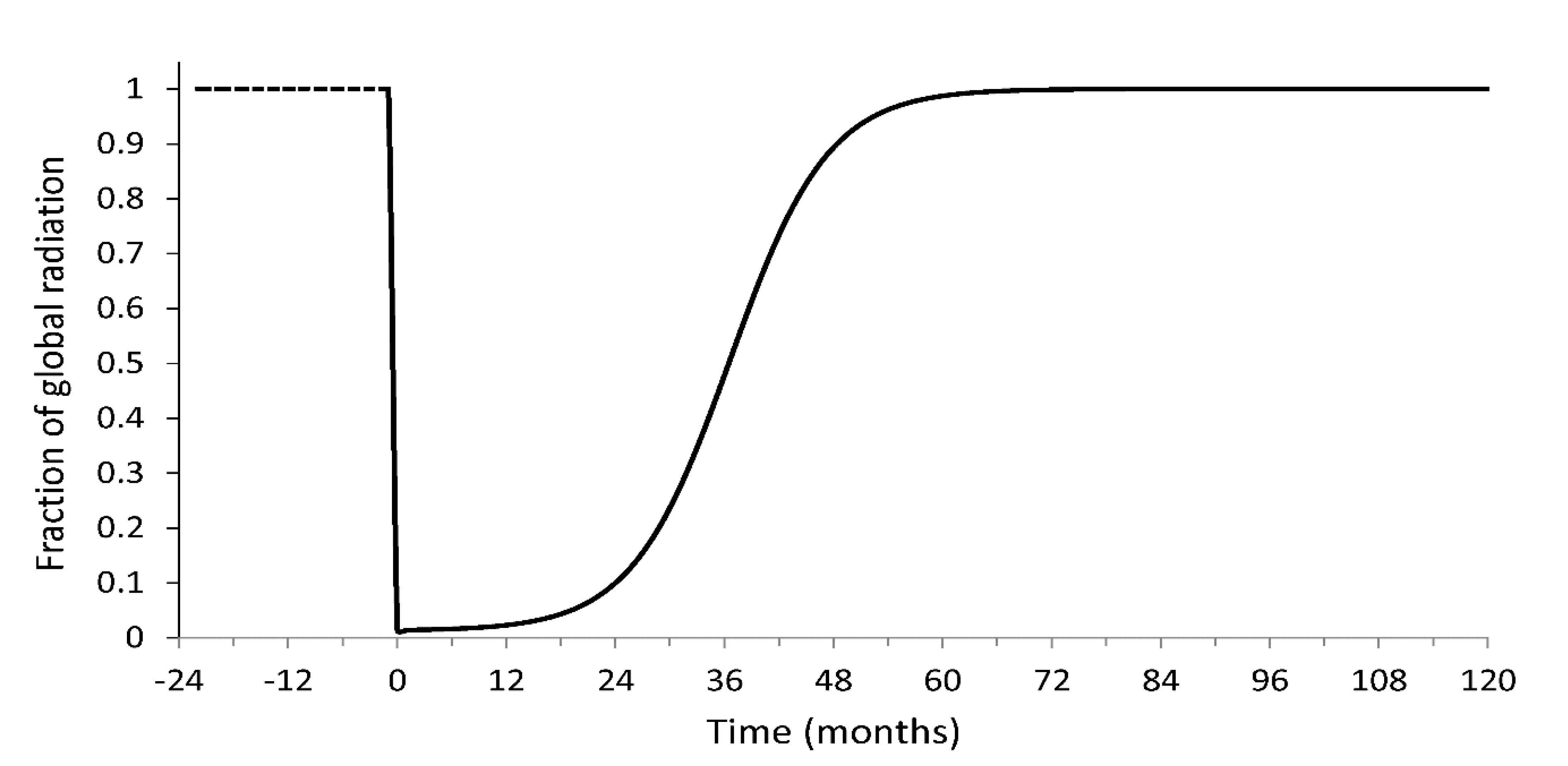
In Figure 1 we show the fraction of the global surface solar radiation (the external forcing), direct plus diffuse and with no clouds, during the impact with respect to its preimpact value. The zero in the time axis corresponds to the moment of the impact. We notice that it takes nearly 4.5 years for the solar radiation to recover its preimpact value. In particular, during the first year, practically no solar radiation reaches the surface.
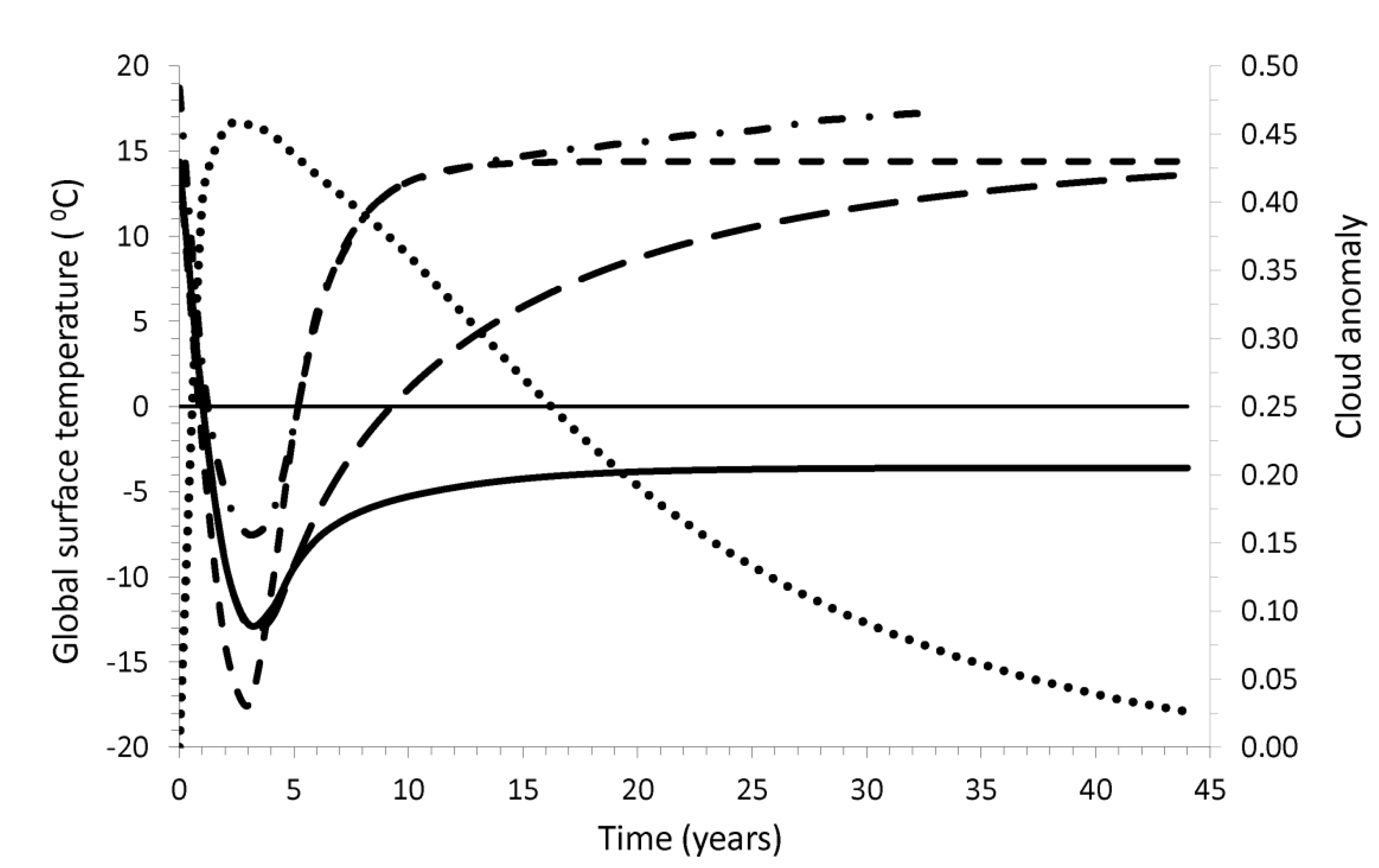
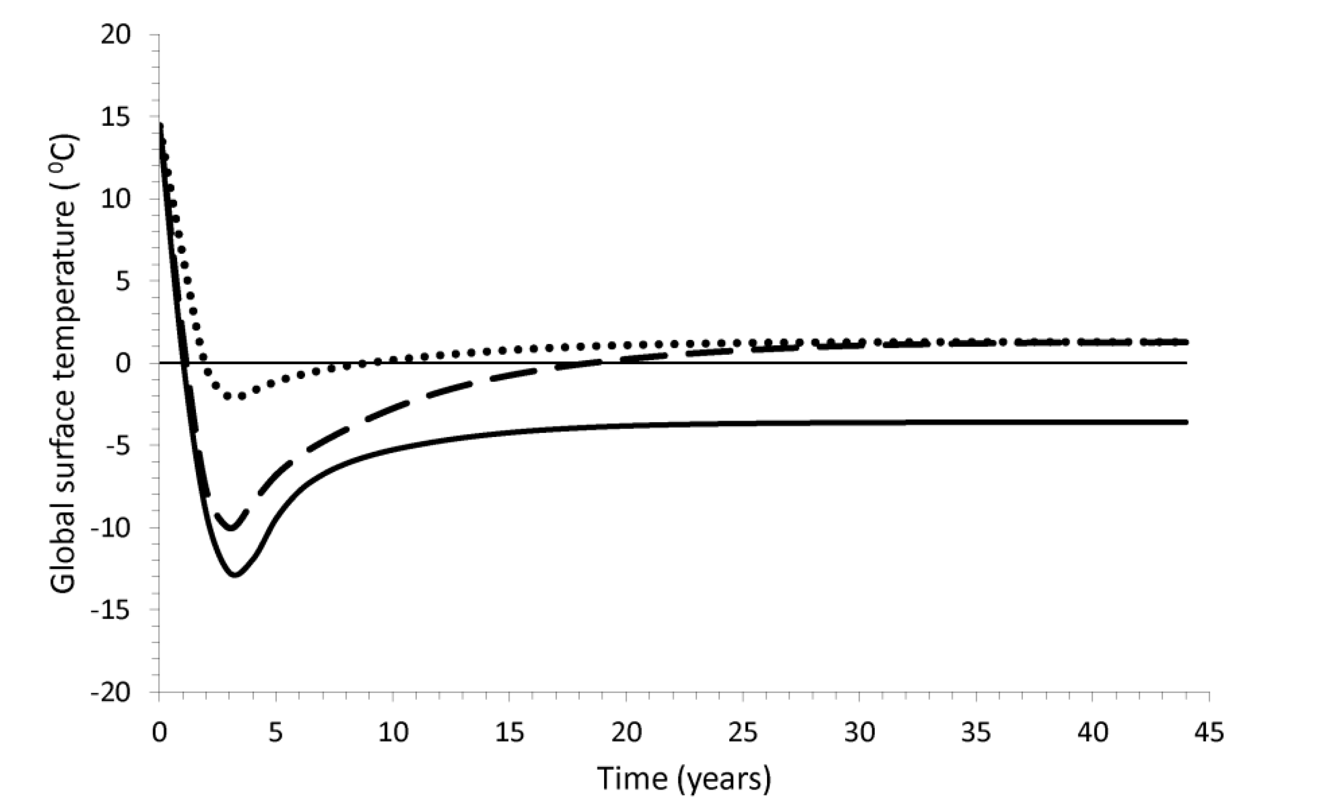
In Figure 2 we show the annual global surface temperature during and after the impact. The preimpact output model temperature, is 14.8 °C, coinciding, as expected, with the present average global temperature. We use three sets of feedback: water vapor; water vapor and clouds; water vapor, clouds, and albedo, associated with the ice cover over continents and oceans. The ice cover is formed due to the cooling produced by stratospheric aerosols. Additionally, the cloud cover anomaly is presented. The model considering only the water vapor produces the fastest preimpact temperature recovery: ~10 years after the impact. Adding the clouds, it takes almost 45 years for the global temperature to recover the preimpact value. Finally, considering the three sets of feedback, the recovery of the preimpact temperature value takes a time longer than 45 years, with a stable value of −3.5 °C. The period of lowest temperatures occurs between 1.5 and 5 years and the deepest phase is reached ~3 years after the impact. The presence of maximum cloudiness, up to ~4 years after the impact, prevents larger cooling due to its greenhouse effect; however, after this time, although the solar radiation at the surface has almost reached its pre-impact value, as shown in Figure 1, the clouds produce an albedo effect that keeps the surface cool for a longer time, which is the reason for the difference between the scenarios with and without clouds. The model found in [33] is also shown in Figure 2.
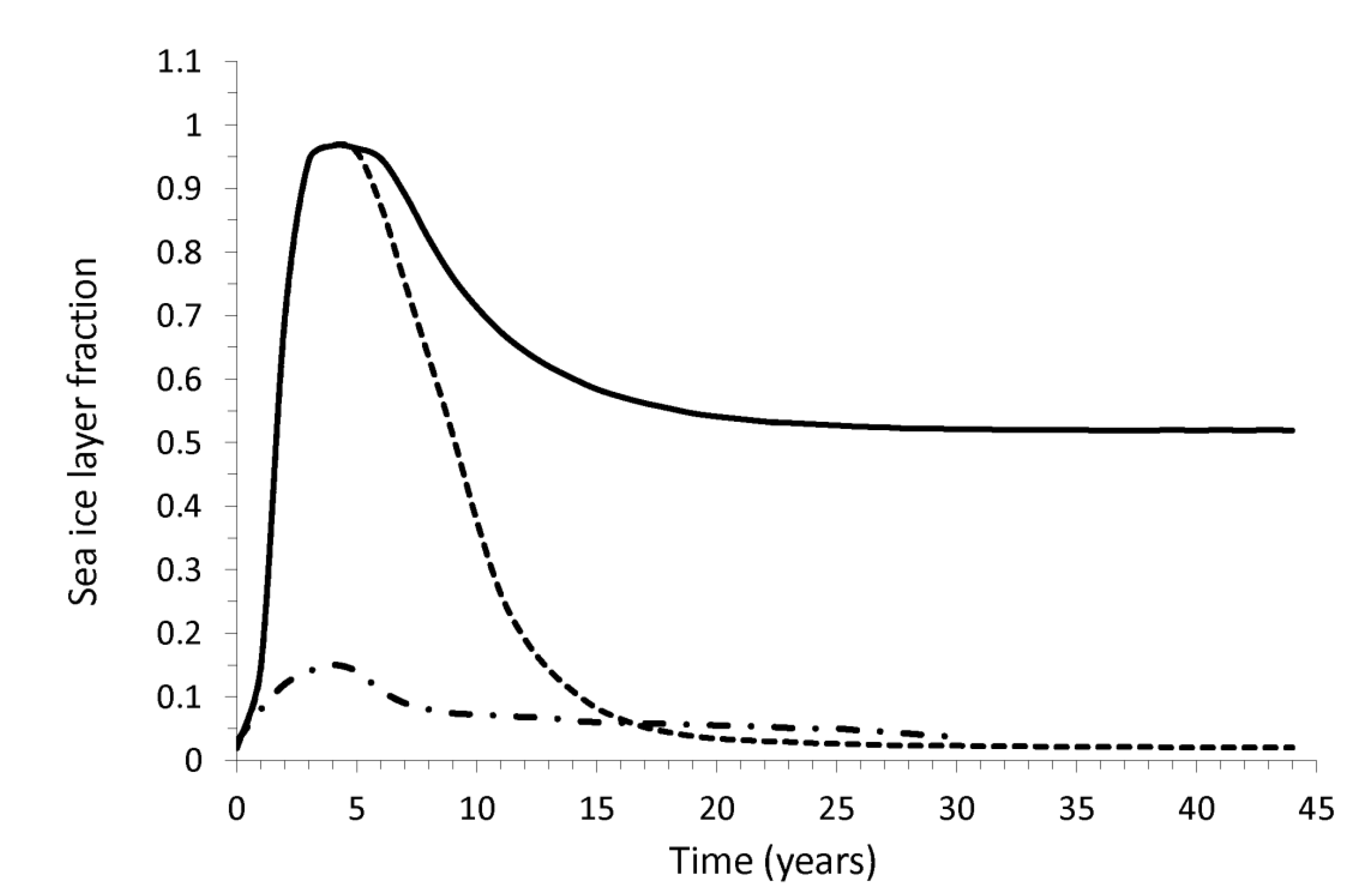
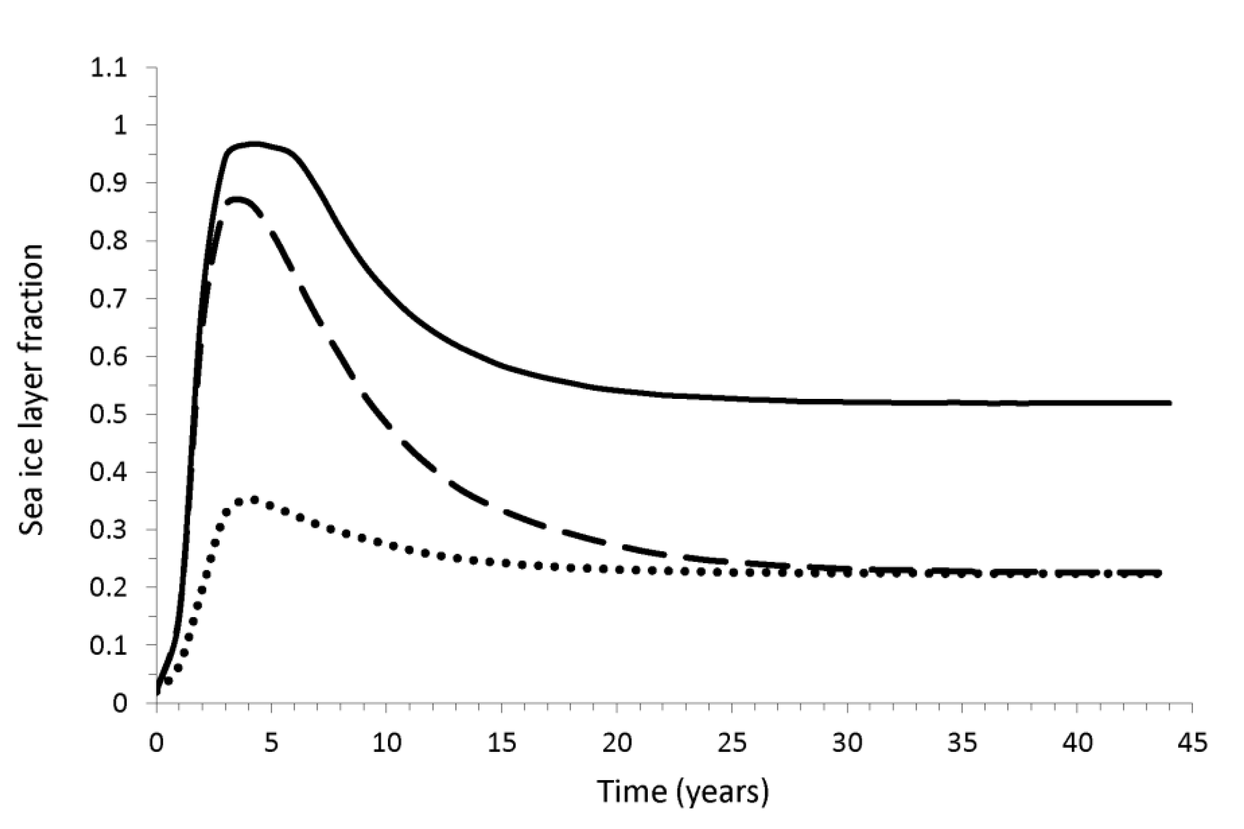
Figure 3 shows the ice fraction over the ocean surface during and after the impact. We consider two feedback scenarios: Water vapor and clouds; water vapor, clouds, and ice cap albedo, formed due to the impact. Considering the first one, the ice covers almost all the ocean surface ~5 years after the impact and its reduction to preimpact values takes around 20 years. Taking the water vapor, clouds and albedo into consideration, for ~6 years the ice covers almost all the ocean surface and after ~25 years such an ice layer is reduced to nearly half of the sea surface, remaining very stable beyond 45 years. The model of [33] is also shown.
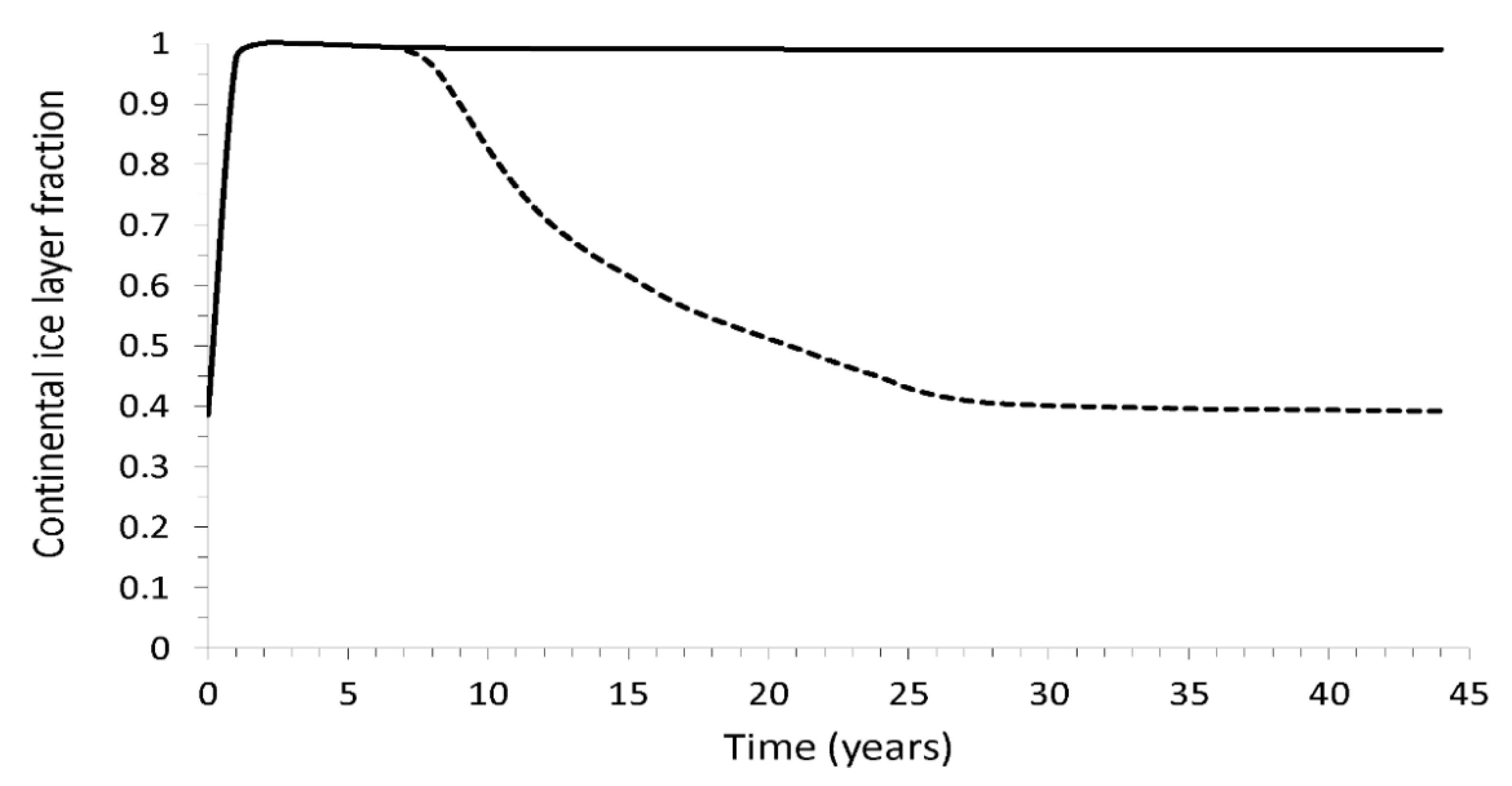
Figure 4 presents the ice fraction over the continental surface during and after the impact. We considered again two scenarios: water vapor and clouds; water vapor, clouds, and the ice cap albedo. If we consider the first scenario, the ice almost covers all the continental surface for 7 years after the impact, and after ~25 years it reduces to nearly 40% of its preimpact values remaining so for a longer time. If we take the water vapor, clouds and albedo, the ice almost covers all the continental surface without reduction beyond 45 years.
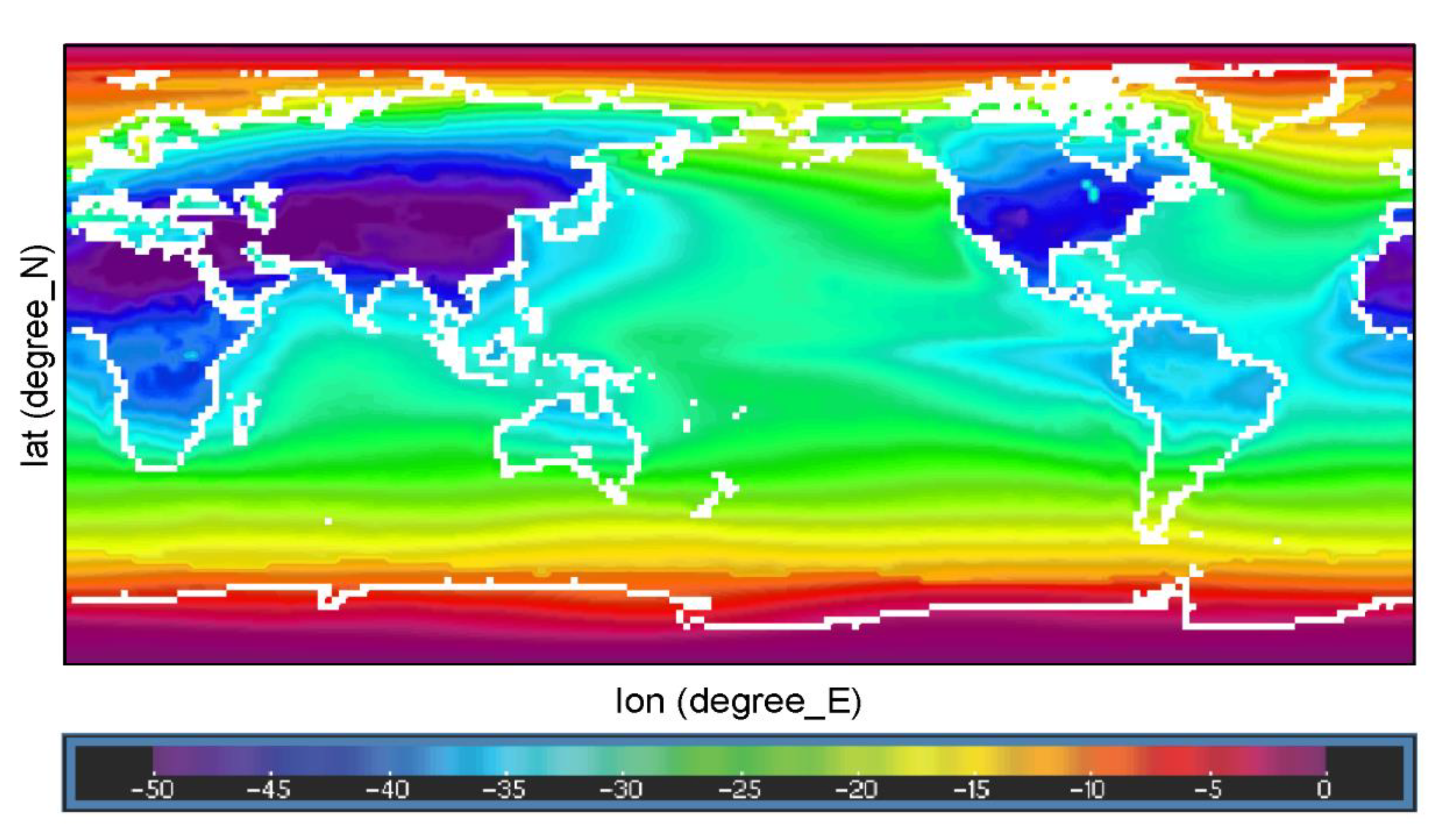
Usually, in climate change simulations, the largest anomalies (either positive or negative) are obtained in July. Figure 5 shows the temperature anomaly in July over the ocean and continental surfaces due to the stratospheric sulphate aerosols 1.5 years after the impact, one of the coldest times, according to Figure 2. The three sets of feedback are included. Almost all the continents, except South America and Oceania, are the coldest places, presenting a temperature anomaly of around −45 °C. The less cold places are the polar regions, with temperature anomalies between −5 °C and 0 °C.
Figure 6 presents the surface continental and oceanic ice cap anomaly 60 years after the impact. The fraction of oceans covered by ice is 0.52, as shown in Figure 3, and the fraction of the continents covered by ice is 0.98, as shown in Figure 4. In the polar regions, after the impact no significant ice was added because they are very dry. This simulation incorporates water vapor, clouds, and ice albedo feedback.
4. Discussion
In this section we compare our results with those in [33], who used a conservative estimate of 100 Gt of S-bearing gases, and included in their simulations the water vapor, cloud, and ice albedo feedback. In the modern scenario we use the same low estimate of 100 Gt of S-atmospheric loading after the impact. Additionally, they used a preimpact value of 18.9 °C, corresponding to the temperature at the end of the Cretaceous, higher than the 14.8 °C found here. They used a CO2 atmospheric concentration of 500 ppm—in our model we used 350.7 ppm. Moreover, they used a TSI of 1354 Wm−2, and in this paper we use a higher value of 1360.8 Wm−2.
The annual global temperature found in [33] is shown in Figure 2. The maximum cooling was −7.5 °C, while our simulation reaches a lower value of −13.5 °C. Nevertheless the changes with respect to the climatic value are not that different—in [33] it is 26.4 °C (it goes from 18.9 to −7.5 °C) and in our case it is 28.3 °C (it goes from 14.8 to −13.5 °C). The temperature in [33] approached its preimpact value after 30 years, whereas in our model the case closest to this behavior is the one including only the water vapor feedback. The lowest temperature in both [33] and our model occurs ~3 years after the impact. In [33], they found that the sea ice surface reached its maximum thickness fraction of ~0.15 approximately 4 years after impact, and ~20 years after impact it almost achieved preimpact values. Our model, considering the water vapor and cloud feedback, and the simulation in [33], coincides in that the ice sea surface fraction almost reaches its preimpact values after 20 years.
As far as we can see, the difference between our results and those in [33] may be attributed to the following effects: the different preimpact temperatures used; the larger greenhouse effect in [33]; an increase of 149.3 ppm in CO2 (the difference between the models’ CO2 concentrations) can further increase the temperature ~2 °C and such an effect remains even in the nearly complete absence of solar radiation; the different TSI values, our value is ~0.5% higher than that in [32], which implies an increased temperature of 0.5 °C. Summarizing, the model in [33] has a higher preimpact temperature than our model. Furthermore, the sea ice model (dynamic–thermodynamic) is used in [33], but in our model, the sea ice mass per unit area and time is proportional to the difference between the latent heat released by vapor condensation, and the latent heat that is yielded by vaporization or sublimation from the surface. In [33], the surface cooling provoked a vigorous ocean mixing, where the resurgence of less cold water prevented the surface ice accumulation. In our model, the sea ice surface is formed by thermodynamic processes. During the period of low solar radiation there was a constant ice surface accumulation. When the solar radiation achieved its preimpact value, the ice albedo feedback had an important roll in maintaining the ice caps for a long time.
Furthermore, after the asteroid impact, we modelled the effect of releasing different quantities of sulphate gases in a proportion of 80% SO2 and 20% SO3. We used water vapor, clouds, and ice albedo feedback. We considered the impacts of loading the atmosphere with 1, 5, and 100 Gt of S-bearing gases. Asteroids that impact the Earth can inject large S quantities into the stratosphere. In [34] the authors calculated the S abundances of carbonaceous asteroids with diameters between 0.1 and 10 km. They found that 0.15 km asteroids contain as much S as the entire modern stratosphere and that the S in a 10 km asteroid is nearly six orders of magnitude larger. Moreover, in [29] the authors found that, for a loading larger than 25 Gt, the magnitude and duration of the maximum radiative forcing is independent of the initial gas release. Following [29], we assume that the released material between 1 and 5 Gt comes only from the asteroid and not from the impact place, while the 100 Gt comes mainly from the target. We use the climate forcing model results, developed in [29], to calculate the radiative forcing. Figure 7 shows the annual global surface temperature. We noticed that the smaller the loading the higher the temperature minimum—around −14, −10, and −2 °C for 100, 5 and 1 Gt, respectively. After ~25 y, the 1 and 5 Gt temperatures reach also a nearly constant value of ~1 °C, compared with the 100 Gt, which keeps the temperature close to −3.5 °C. However, in the three cases, the low temperatures go beyond 45 y after the impact; therefore, a semi-permanent shift of climate seems to be achieved. Figure 8 shows the ice surface fraction over the oceans. Again, the smaller the loading, the smaller the ice fraction over the ocean. The maximum ice coverage occurs within the first 5 years after the impact—almost all the ocean surface, ~0.85% and ~0.35% for 100, 5 and 1 Gt, respectively. After ~25 years, such an ice layer is reduced to nearly half of the sea surface, and ~0.20% of the sea surface for 100, and both 5 and 1 Gt, respectively. The ice fraction for the three cases remains very stable beyond 45 years. Again, this suggests a semi-permanent shift of climate. In [29], the authors modeled the climate forcing for S-loadings between 1 to 300 Gt, and for the Pitanubo as a loading lower limit. They found that the radiative forcing associated with Pitanubo is around two orders of magnitude lower than that associated to the 1 Gt loading. Its climatic effect only lasted for about 2 years; therefore, no long-term shift in the climate system occurred.
As indicated above, we assume that the present day asteroid and the Chicxulub-type object impacted in similar places—a partially submerged platform constituting a thick sequence (3 km) of carbonates and sulphate evaporites. Nevertheless, there are other sulphate evaporite-rich provinces in the world, such as Solikamsk in the Urals in Russia, Soligorsk in Bielorusia, Saskatchewan and New Brunswick in Canada, or Stassfurt and Hannover in Germany. In Spain, they are in Suria-Cardona, Cabezón de la Sal, and, in general, in marine basins, such as the Guadalquivir depression. In all these places, a Chicxulub-like impact would probably produce a similar climatic effect. However, if the asteroid hits a granite craton—for instance North America, Africa, or northern Asia—the sulphate loading would come only from the asteroid, represented in Figure 7 and Figure 8. Moreover, if the impact is on the oceans, and if the oceanic crust does not have sulphate evaporite sediments, the loading would be mainly water vapor. In this case, most water vapor would be in the troposphere, and the vapor in the stratosphere would contribute to the aerosol formation of S acid, as the S loading would be due only to the asteroid, again, shown in Figure 7 and Figure 8, which represent the climatic effect. If the evaporites are mainly constituted by minerals other than sulphates, then we also consider that the sulphates come from the asteroid.
5. Conclusions
A large-size asteroid event on our planet occurs, on average, every ten to hundred million years. One of those objects struck the Earth around 66.04 million years ago. Therefore, such an event may happen in the present. Here, we simulated the associated sudden climate change, with respect to the present, of a Chicxulub-like asteroid impacting a similar sulfur-rich target. For this purpose we used a thermodynamic climate model that includes the feedback caused by water vapor, cloudiness (by greenhouse and albedo effects), and cryosphere, to calculate global cooling due to aerosols produced by the asteroid impact on the Earth. We found that:
It takes nearly 4.5 years for the solar radiation reaching the surface to recover its preimpact value. In particular, during the first year practically no solar radiation reaches the surface. The recovery of the preimpact temperature takes beyond 45 years. The coldest temperatures are found between 1.5 and 5 years after the impact and the lowest is around −14 °C below the preimpact temperature. The July surface oceanic and continental temperature anomalies, 1.5 years after the impact, become one of the coldest, compared to preimpact temperatures. Almost all the continents, except South America and Oceania, have temperature anomalies of −45 °C. The polar regions show lower temperature anomalies, between −5 and 0 °C.
Our most remarkable results are: For ~6 years the ice extends over almost all the ocean surface, and after ~25 years it covers nearly half of the surface, remaining so beyond 45 years. The continental ice remains without reduction beyond 45 years. Sixty years after the impact, the oceanic surface fraction covered by ice is 0.52 and the continental fraction is 0.98. We also modeled the effect of smaller quantities of sulphur released after asteroid impacts, concluding that an instantaneous, large climatic perturbation, attributed to a loading range, can lead to a semi-permanent shift in the climate system.
Author Contributions
Conceptualization, V.M.M. and R.G.; methodology, B.M.; software, M.P. and V.M.M.; validation, B.M. and R.G.; formal analysis, V.M.M.; investigation, B.M.; data curation, V.M.M. and M.P.; writing—original draft preparation, B.M.; writing—review and editing, B.M. All authors have read and agreed to the published version of the manuscript.
Funding
This research received no external funding.
Acknowledgments
We would like to acknowledge Alejandro Aguilar for the help in preparing the figures.
Conflicts of Interest
The authors declare no conflict of interest.
References
- Alvarez, L.W.; Alvarez, W.; Asaro, F.; Michel, H.V. Extraterrestrial cause of the Cretaceous–Tertiary extinction. Science 1980, 208, 1095–1108. [Google Scholar] [CrossRef] [Green Version]
- Bambach, R.K. Phanerozoic biodiversity mass extinctions. Annu. Rev. Earth Planet. Sci. 2006, 34, 127–155. [Google Scholar] [CrossRef]
- Schulte, P.; Alegre, L.; Arenillas, I.; Arz, J.A.; Barton, P.J.; Bown, P.R.; Bralower, T.J.; Christeson, G.L.; Claeys, P.; Cockell, C.S. The chicxulub asteroid impact and mass extinction at the cretaceous-paleogene boundary. Science 2010, 327, 1214–1218. [Google Scholar] [CrossRef] [PubMed] [Green Version]
- Robertson, D.S.; Lewis, W.M.; Sheehan, P.M.; Toon, O.B. K-Pg extinction patterns in marine and freshwater environments: The impact winter model. J. Geophys. Res. Biogeosci. 2013, 118, 1006–1014. [Google Scholar] [CrossRef]
- Collins, G.S.; Melosh, H.J.; Marcus, R.A. Earth impact effects program: A web-based computer program for calculating the regional environmental consequences of a meteoroid impact on Earth. Meteorit. Planet. Sci. 2005, 40, 817–840. [Google Scholar] [CrossRef] [Green Version]
- DePalma, R.A.; Smit, J.; Burnham, D.A.; Kuiper, K.; Manning, P.L.; Oleinik, A.; Larson, P.; Maurrasse, F.J.; Vellekoop, J.; Richards, M.A.; et al. A seismically induced onshore surge deposit at the KPg boundary, North Dakota. PNAS 2019, 116, 8190–8199. [Google Scholar] [CrossRef] [PubMed] [Green Version]
- Robertson, D.S.; Lewis, W.M.; Sheehan, P.M.; Toon, O.B. K-Pg extinction: Reevaluation of the heat-fire hypothesis. J. Geophys. Res. Biogeosci. 2013, 118, 329–336. [Google Scholar] [CrossRef]
- Gulick, S.P.S.; Bralower, T.J.; Ormö, J.; Hall, B.; Grice, K.; Schaefer, B.; Lyons, S.; Freeman, K.H.; Morgan, J.V.; Artemieva, N.; et al. The first day of the Cenozoic. PNAS 2019, 116, 19342–19351. [Google Scholar] [CrossRef] [PubMed] [Green Version]
- Bourgeois, J.; Hansen, T.A.; Wiberg, P.L.; Kauffman, E.G. A tsunami deposit at the Cretaceous-Tertiary boundary in Texas. Science 1988, 241, 567–570. [Google Scholar] [CrossRef]
- Ward, S.N.; Asphaug, E. Asteroid impact sunami: A probabilistic hazard assessment. Icarus 2000, 145, 64–78. [Google Scholar] [CrossRef]
- Bralower, T.J.; Paull, C.K.; Leckie, R.M. The Cretaceous-Tertiary boundary cocktail: Chicxulub impact triggers margin collapse and extensive sediment gravity flows. Geology 1998, 26, 331–334. [Google Scholar] [CrossRef] [Green Version]
- Koeberl, C.; Ivanov, B.A. Asteroid impact effects on Snowball Earth. Meteorit Planet. Sci. 2019, 54, 2273–2285. [Google Scholar] [CrossRef] [Green Version]
- Poveda, A.; Herrera, M.A.; García, J.L.; Curioca, K. The diameter distribution of Earth-crossing asteroids. Planet. Space Sci. 1999, 47, 679–685. [Google Scholar] [CrossRef]
- Renne, P.R.; Deino, A.L.; Hilgen, F.J.; Kuiper, K.F.; Mark, D.F.; Mitchell, W.S.; Morgan, L.E.; Mundil, R.; Smit, J. Time scales of critical events around the Cretaceous-Paleogene boundary. Science 2013, 339, 684–687. [Google Scholar] [CrossRef] [PubMed] [Green Version]
- Artemieva, N.; Morgan, J.; Expedition 364 Science Party. Quantifying the release of climate-active gases by large meteorite impacts with a case study of Chicxulub. Geophys. Res. Lett. 2017, 44, 10180–11018. [Google Scholar] [CrossRef] [Green Version]
- Collins, G.S.; Patel, N.; Davison, T.M.; Rae, A.S.P.; Morgan, J.V.; Gulick, S.P.S.; IODP-ICDP Expedition 364 Science Party and Third-Party Scientists. A steeply-inclined trajectory for the Chicxulub impact. Nat. Commun 2020, 11, 1480. [Google Scholar] [CrossRef]
- Schoene, B.; Samperton, K.M.; Eddy, M.P.; Keller, G.; Adatte, T.; Bowring, S.A.; Khadri, S.F.R.; Gertsch, B. U-Pb geochronology of the Deccan Traps and relation to the end-Cretaceous mass extinction. Science 2015, 347, 182–184. [Google Scholar] [CrossRef]
- Hull, P.M.; Bornemann, A.; Penman, D.E.; Henehan, M.J.; Norris, R.D.; Wilson, P.A.; Blum, P.; Alegret, L.; Batenburg, S.J.; Bown, P.R.; et al. On impact and volcanism across the Cretaceous-Paleogene boundary. Science 2020, 367, 266–272. [Google Scholar] [CrossRef] [Green Version]
- Artemieva, N.; Morgan, J. Global K-Pg layer deposited from a dust cloud. Geophys. Res. Lett. 2020, 47, e2019GL086562. [Google Scholar] [CrossRef]
- Cuvey, C.; Thompson, S.L.; Weissman, P.R.; MacCracken, M.C. Global climatic effects of atmospheric dust from an asteroid or comet impact on Earth. Glob. Planet. Chang. 1994, 9, 263–273. [Google Scholar] [CrossRef]
- Pierazzo, E.; Kring, D.A.; Melosh, H.J. Hydrocode simulation of the Chicxulub impact event and the production of climatically active gases. J. Geophys. Res. 1998, 103, 28607–28625. [Google Scholar] [CrossRef]
- Pope, K.O. Impact dust not the cause of the Cretaceous-Tertiary mass extinction. Geology 2002, 30, 99–102. [Google Scholar] [CrossRef]
- Adem, J.; Mendoza, V.M.; Ruíz, A.; Villanueva, E.E.; Garduño, R. Recent numerical experiments on three-months extended and seasonal weather prediction with a thermodynamic model. Atmósfera 2000, 13, 53–83. [Google Scholar]
- Mendoza, V.M.; Mendoza, B.; Garduñ, R.; Cordero, G.; Pazos, M.; Cervantes, S.; Cervantes, K. Thermodynamic simulation of the seasonal cycle of temperature, pressure and ice caps on Mars. Atmósfera 2020, in press. [Google Scholar] [CrossRef]
- Mendoza, V.M.; Mendoza, B.; Garduño, R.; Villanueva, E.E.; Adem, J. Solar activity cloudiness effect on NH warming for 1980–2095. Adv. Space Res. 2016, 57, 1373–1390. [Google Scholar] [CrossRef]
- Mendoza, V.M.; Villanueva, E.E.; Garduñ, R.; Sánchez-Meneses, O. Atmospheric emissivity with clear sky computed by E-Trans/HITRAN. Atmos. Environ. 2017, 155, 174–188. [Google Scholar] [CrossRef]
- Adem, J. Parametrization of atmospheric humidity using cloudiness and temperature. Mont. Weath. Rev. 1967, 95, 83–88. [Google Scholar] [CrossRef] [Green Version]
- Gerstl, S.A.W.; Zardecki, A. Effects of aerosols on photosynthesis. Nature 1982, 300, 436–437. [Google Scholar] [CrossRef]
- Pierazzo, E.; Hahmann, A.N.; Sloan, L. Chicxulub and climate: Radiative perturbations of impact-produced S-bearing gases. Astrobiology 2003, 3, 99–118. [Google Scholar] [CrossRef]
- Available online: http://co2now.org/Current-CO2/CO2-Now/noaa-maunaloa-co2-data.html (accessed on 14 July 2020).
- Kopp, G.; Lean, J. A new, lower value of total solar irradiance: Evidence and climate significance. Geophys. Res. Lett. 2011, 38, L01706. [Google Scholar] [CrossRef] [Green Version]
- Pinto, J.P.; Turco, R.P.; Toon, O.B. Self-limiting physical and chemical effects in volcanic eruption clouds. J. Geophys. Res. 1989, 94, 11165–11174. [Google Scholar] [CrossRef]
- Brugger, J.; Feulner, G.; Petri, S. Baby, it’s cold outside: Climate model simulations of the effects of the asteroid impact at the end of the Cretaceous. Geophys. Res. Lett. 2017, 44, 419–427. [Google Scholar] [CrossRef]
- Kring, D.A.; Melosh, H.J.; Hunten, D.M. Impact-induced perturbations of atmospheric sulfur. Earth Planet. Sci. Lett. 1996, 140, 201–212. [Google Scholar] [CrossRef]
Figure 1.
Fraction of the surface solar radiation reaching the surface during and after the asteroid impact. The zero in the time axis represents the moment of the impact.
Figure 1.
Fraction of the surface solar radiation reaching the surface during and after the asteroid impact. The zero in the time axis represents the moment of the impact.

Figure 2.
Annual global surface temperature during and after the impact. Three sets of feedback are used: water vapor (short-dashed curve); water vapor and clouds (long-dashed curve); water vapor, clouds, and ice albedo (solid curve). The modeled fractional cloud cover anomaly is the dotted curve. The simulation in [33], including these three types of feedback, is the dashed–dotted curve.

Figure 3.
Ice surface fraction over the oceans during and after the impact. Calculated using water vapor and cloud feedback (short-dashed curve) and adding the ice albedo (solid curve). The result in [33] is the dashed–dotted curve.
Figure 3.
Ice surface fraction over the oceans during and after the impact. Calculated using water vapor and cloud feedback (short-dashed curve) and adding the ice albedo (solid curve). The result in [33] is the dashed–dotted curve.

Figure 4.
Ice surface fraction over the continents during and after the impact. Calculated using water vapor and cloud feedback (short–dashed curve) and adding the ice albedo (solid curve).
Figure 4.
Ice surface fraction over the continents during and after the impact. Calculated using water vapor and cloud feedback (short–dashed curve) and adding the ice albedo (solid curve).

Figure 5.
July surface temperature anomaly 1.5 years after the impact, one of the coldest times. Calculated using water vapor, clouds, and ice albedo feedback.
Figure 5.
July surface temperature anomaly 1.5 years after the impact, one of the coldest times. Calculated using water vapor, clouds, and ice albedo feedback.

Figure 6.
Continental and oceanic ice cap anomaly 60 years after the impact calculated using water vapor, cloud, and ice albedo feedback. Color code: regions with ice thickness of more than 1 m, from gray (thinner ice cap) to white (thicker ice cap); regions with no ice or ice thickness less than 1 m, black.

Figure 7.
Annual global surface temperature during and after various asteroid impacts. Atmospheric S loading of: 1 Gt (pointed curve), 5 Gt (dashed curve), and 100 Gt (solid curve).
Figure 7.
Annual global surface temperature during and after various asteroid impacts. Atmospheric S loading of: 1 Gt (pointed curve), 5 Gt (dashed curve), and 100 Gt (solid curve).

Figure 8.
Ice surface fraction over the oceans during and after various asteroid impacts. Atmospheric S loading of: 1 Gt (pointed curve), 5 Gt (dashed curve), and 100 Gt (solid curve).
Figure 8.
Ice surface fraction over the oceans during and after various asteroid impacts. Atmospheric S loading of: 1 Gt (pointed curve), 5 Gt (dashed curve), and 100 Gt (solid curve).

© 2020 by the authors. Licensee MDPI, Basel, Switzerland. This article is an open access article distributed under the terms and conditions of the Creative Commons Attribution (CC BY) license (http://creativecommons.org/licenses/by/4.0/).
Share and Cite
MDPI and ACS Style
Mendoza, V.M.; Mendoza, B.; Garduño, R.; Pazos, M. Modelling the Present Global Terrestrial Climatic Response Due to a Chicxulub-Type Asteroid Impact. Atmosphere 2020, 11, 747. https://doi.org/10.3390/atmos11070747
AMA Style
Mendoza VM, Mendoza B, Garduño R, Pazos M. Modelling the Present Global Terrestrial Climatic Response Due to a Chicxulub-Type Asteroid Impact. Atmosphere. 2020; 11(7):747. https://doi.org/10.3390/atmos11070747
Chicago/Turabian StyleMendoza, Víctor M., Blanca Mendoza, René Garduño, and Marni Pazos. 2020. "Modelling the Present Global Terrestrial Climatic Response Due to a Chicxulub-Type Asteroid Impact" Atmosphere 11, no. 7: 747. https://doi.org/10.3390/atmos11070747
Note that from the first issue of 2016, this journal uses article numbers instead of page numbers. See further details here.