Strategies for Assimilating High-Density Atmospheric Motion Vectors into a Regional Tropical Cyclone Forecast Model (HWRF)


Space Science and Engineering Center, Madison, WI 53706, USA
*
Author to whom correspondence should be addressed.
Atmosphere 2020, 11(6), 673; https://doi.org/10.3390/atmos11060673
Submission received: 28 May 2020
/
Revised: 22 June 2020
/
Accepted: 23 June 2020
/
Published: 26 June 2020
(This article belongs to the Special Issue Modeling and Data Assimilation for Tropical Cyclone Forecasts)
Abstract
:In recent years, atmospheric numerical modeling frameworks and satellite observing systems have both undergone significant advances. While these developments offer considerable potential for improving forecasts of high-impact weather events such as tropical cyclones (TC), much work remains to be done regarding the targeted processing and optimal use of observations now becoming available with high spatiotemporal resolution. Using the 2019 version of NCEP’s HWRF model, we explore several different strategies for the assimilation of TC-scale, high-density atmospheric motion vectors (AMVs) derived from the new-generation GOES-R series of geostationary satellites. Using 2017’s Atlantic Hurricane Irma as a case study, we examine the HWRF forecast impacts of observation pre-processing, including thinning and adjustments to observation errors. It is demonstrated that enhanced vortex-scale GOES-16 AMVs contribute to notable improvements in HWRF track forecast error compared to a baseline control experiment that does not incorporate the high-density AMVs. Impacts on TC intensity and structure (i.e., wind radii) forecast errors are less robust, but results from the optimization experiments suggest that further work (both with regard to data assimilation strategies and advancements in the methods themselves) should lead to improvements in these forecast variables as well.
1. Introduction
Tropical cyclones (TCs) are among the most spectacular of natural phenomena, and, in terms of their potential to impact society on vast socioeconomic scales, they remain one of mankind’s greatest forecast challenges. In the average year, about 80 to 90 TCs will form over the Atlantic, Pacific, and Indian oceans [1], and, of these, a smaller number will develop into intense cyclones that menace shipping lanes and threaten coastal areas with high winds, storm-surge inundation, and freshwater flooding from rainfall accumulations that can exceed 1 m in extreme cases, such as 2017′s Hurricane Harvey [2]. As coastal populations continue to increase in the 21st century, accurate projections of TC track, intensity, and structure will become more critical than ever.
To meet this challenge, continued development of numerical weather prediction (NWP) and data assimilation techniques (DA) are necessary. NWP models such as the National Centers for Environmental Prediction (NCEP) Hurricane Weather Research and Forecasting Model (HWRF) [3] and its accompanying DA system have undergone tremendous development during the past decade. Increases in model resolution, more realistic parameterizations of sub-grid-scale phenomena (cumulus convection, cloud microphysics, boundary layer fluxes of enthalpy and momentum), and increasingly sophisticated ensemble-based DA techniques have resulted in an increase in both TC track and intensity forecast skill [4].
However, continued NWP and DA developments are insufficient in themselves to meet the TC forecast challenges of the future. Indeed, the emergence of improved observations, particularly those deriving from recently launched spaceborne platforms such as the new-generation GOES-R and Himawari series of geosynchronous satellites, must be entrained into the operational DA process to leverage their unique ability to provide near-continuous surveillance of the TC and its environment at spatial scales approaching those provided by in-situ platforms such as airborne reconnaissance aircraft. One such observation type is produced by the derivation of tropospheric wind estimates, more commonly known as atmospheric motion vectors (AMVs). Previous work by the authors of [5] demonstrated that a notional enhanced AMV dataset generated from rapid-scan GOES-14 imagery had generally modest positive impacts on HWRF forecasts of three TCs from the 2012 and 2014 Atlantic hurricane seasons. Other recent studies also found generally positive forecast impacts, indicating the promise of AMV observations when directly assimilated into a regional-scale hurricane model [6,7,8,9,10,11].
The Advanced Baseline Imager (ABI) onboard the new-generation GOES-16 satellite is providing high-spatial- and temporal-resolution images that can be targeted on North Atlantic TCs. In addition to the routine full-disk scan every 10 min and Continental U.S. (CONUS) scanning every 5 min, the ABI also has a flexible mesoscale scan mode for targeting limited domains in one-minute intervals. This “meso sector” is moveable and can be focused on a TC center with 10° × 10° domain coverage that follows the storm motion with time. By using this one-minute ABI imagery, specially tailored automated algorithms have been developed to produce enhanced, high-resolution AMVs during a targeted TC event [12]. These spatially and temporally dense AMV datasets can provide critical dynamical information on the targeted storm and its near environment [5].
Here, the HWRF model is used to test a few assimilation strategies for these high-resolution AMVs and study the impact on hurricane forecasts with a view toward optimizing their operational use in HWRF (and future modeling systems such as the Hurricane Analysis and Forecast System, or HAFS). We present results documenting assimilation, experimentation and impact of specially reprocessed GOES-16 AMVs on HWRF forecasts of Hurricane Irma (2017). The remainder of the paper is organized as follows: Section 2 provides details of the modeling and DA system, the case study chosen as well as the accompanying AMV dataset, and a description of the experiment design. Section 3 presents the results of the experiments, and Section 4 and Section 5 give a discussion of the results and a summary of the study findings, respectively.
2. Experiments
2.1. The HWRF Modeling and DA System
All simulations in this study were performed with NCEP’s HWRF modeling and DA system retrieved from the HWRF developer’s branch on 11 April 2019 (the publicly available version is available from the Developmental Testbed Center [13]). It represents substantially the core of the HWRF system deployed operationally for the 2019 hurricane season (hereafter referred to as H219). HWRF employs a triply nested grid. The outer parent domain (hereafter referred to as d01) comprises 390 grid points east–west and 780 grid points north–south at a spacing of 0.099° and remains fixed for the duration of the forecast. Two smaller domains (hereafter referred to as d02 and d03) move with the TC and comprise 268 east–west and 538 north–south points with grid spacing of 0.033° and 0.011°, respectively. All domains have 75 points in the vertical, and the model top is set at 10 hPa. Physics parameterizations on all grids include the scale-aware simplified Arakawa–Schubert cumulus scheme [14], Ferrier high-resolution microphysics [15,16], the Rapid Radiative Transfer Model for GCM applications (RRTMG) longwave and shortwave radiation scheme [17], the Geophysical Fluid Dynamics Laboratory (GFDL) surface layer scheme [18], and the NCEP Global Forecast System (GFS) hybrid eddy-diffusivity mass-flux (Hybrid-EDMF) planetary boundary layer (PBL) scheme [19]. To simulate air–sea interaction and the impact of sea-surface temperature (SST) cooling on the evolution of the TC, HWRF is coupled to the Princeton Ocean Model for use with TCs (POM-TC) [20].
TC analysis and forecasting with HWRF is a multi-step process that begins with the interpolation of GFS analysis fields to d01 at the beginning of each 6-h analysis cycle (i.e., no DA is performed on d01). The storm-following domains, d02 and d03, are initialized from the GDAS 6-h forecast, and observations are assimilated (including AMVs) over a +/−3-h window centered on each analysis time. The first-guess fields on d02 and d03 are further modified in a number of ways depending on whether the analysis cycle is for a cold start (i.e., the first cycle of a cycling DA experiment) or a warm start (i.e., cycles for which a previous forecast serves as the first guess). For the initial cycle, the GDAS 6-h forecast is modified by the addition of a bogus vortex; subsequent cycles employ vortex relocation and structure correction (i.e., modification of the wind and mass fields) to bring them into better agreement with the observed values of maximum wind and critical wind radii as specified in the NCEP TC-Vitals message valid at the analysis time [3]. For this study, analysis cycling occurs every 6 h at the standard synoptic time (i.e., 00, 06, 12, and 18 UTC).
The DA component of the HWRF system uses the Environmental Modeling Center (EMC) version of the Gridpoint Statistical Interpolation (GSI) code checked out from the EMC repository [21] on 11 April 2019. Specifically, when tail-Doppler radar (TDR) (see, e.g., [22]) observations are available, the two-way hybrid EnKF-GSI algorithm is employed, meaning that the forecast error covariance is given by a blend of static NCEP covariance and the sample covariance provided by a 40-member ensemble of 6-h high-resolution HWRF forecasts. When TDR observations are not available, the forecast error covariance is computed using the one-way hybrid method (i.e., a blend of the static NCEP covariance and the sample covariance provided by the NCEP GFS 80-member ensemble). All data assimilated in this study come from the suite of operationally available BUFR files and include observations from both conventional (radiosonde, ship and surface airways reports, etc.), airborne (TDR, flight-level reconnaissance, etc.) and satellite (SSMIS and AMSU-A radiances, etc.) platforms. The one exception to this rule involves the reprocessed GOES-16 AMVs which are the focus of this study.
Further details on HWRF, GSI and all components of the modeling system can be found in the most recent version of the HWRF scientific documentation [3]. All simulations and analysis were carried out on the NOAA Jet supercomputer located in Boulder, CO.
2.2. Hurricane Irma (2017)
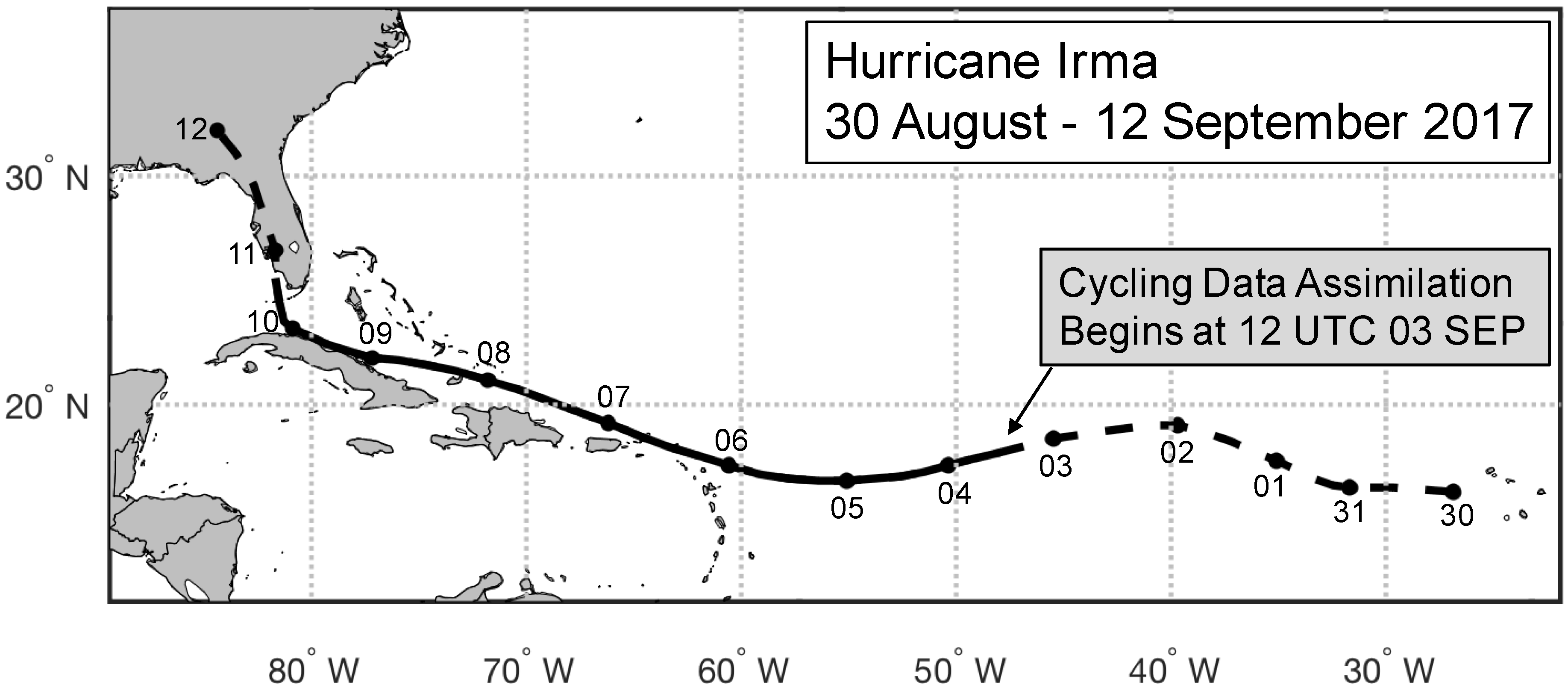
Hurricane Irma was one of several destructive hurricanes to impact the Atlantic basin during the 2017 season, spreading a swath of destruction from the Leeward and Virgin Islands to the Bahamas, Cuba and the United States. In the United States alone, Irma resulted in 92 fatalities and damage from wind, storm surge and freshwater flooding is estimated at 50 billion US dollars [23]. The disturbance that would become Irma moved off the west coast of Africa on 27 August and developed into a tropical depression on 30 August while situated west of the Cape Verde Islands. From there, it tracked between west-southwestward and west-northwestward before finally turning north over the Florida Straits toward its landfall in the United States (Figure 1).
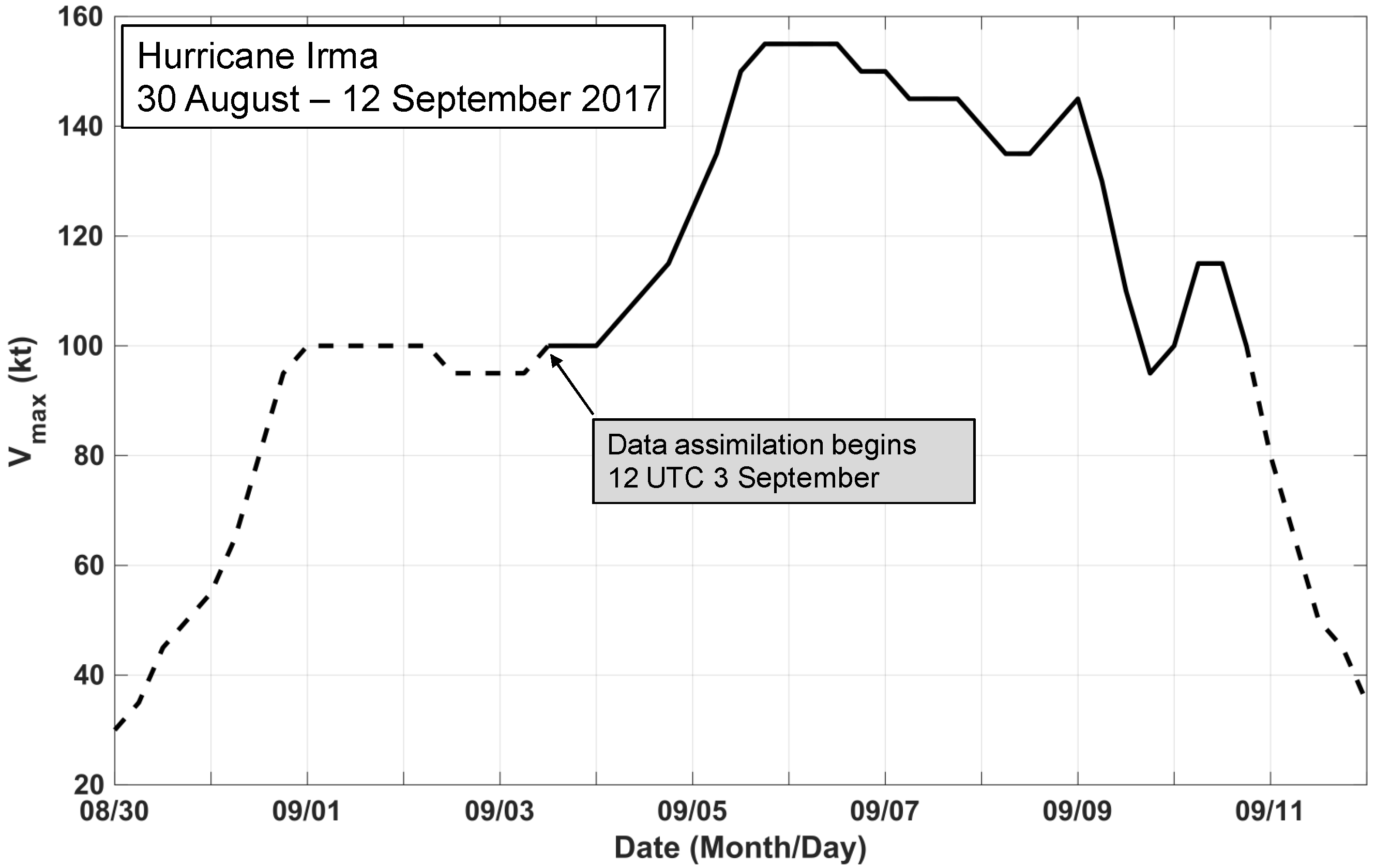
Irma rapidly intensified into a major hurricane on 1 September while over the eastern tropical Atlantic (Figure 2). An eyewall-replacement cycle temporarily prevented any further increase in strength, but, beginning on 4 September, another period of rapid intensification began and lasted until midday on 5 September, by which time Irma had strengthened into a formidable category-5 hurricane with maximum sustained winds of 155 kt. Incredibly, Irma maintained category-5 intensity for 60 h until a second eyewall replacement cycle and associated dry-air intrusion [23] resulted in a weakening phase that lasted until 8 September. Irma then briefly regained category-5 intensity before making landfall on the north coast of Cuba. A day and a half later, Irma made landfall near Marco Island, Florida as a category-3 hurricane and later dissipated over southern Georgia, bringing its long and destructive history to an end.
Aside from its historic destructiveness, Irma’s sequence of multiple rapid intensification events and eyewall replacement cycles make it an ideal case for study. TCs which undergo rapid intensity change and/or eyewall replacement cycles often present exquisite challenges for numerical guidance. Irma was no exception [23]. In addition, the newly launched GOES-16 was placed in pre-operational check-out mode by NOAA/NESDIS during the 2017 Atlantic TC season. The flexible meso-scan imaging mode was activated and began targeting Irma on 3 September and continued following it for the duration of the storm.
2.3. GOES-16 AMVs
For this study, AMV datasets were reprocessed by the University of Wisconsin Cooperative Institute for Meteorological Satellite Studies (UW/CIMSS) from GOES-16 ABI rapid scan imagery beginning on 3 September for Hurricane Irma (2017). Special processing strategies were imposed to enhance AMV coverage and maximize the information content to resolve the scales of the flow fields associated with the storm vortex and its near environment. Crucial to obtaining these observations is the continuous 1-min image sampling over targeted storms as mentioned above. In addition to using 1-min image triplets in the cloud tracking process, modifications for enhanced AMV coverage (vs. routine full-disk processing) included increasing the target density, reducing the minimum gradient required for target identification, disabling stringent coherency requirements, and relaxing QC constraints [12].
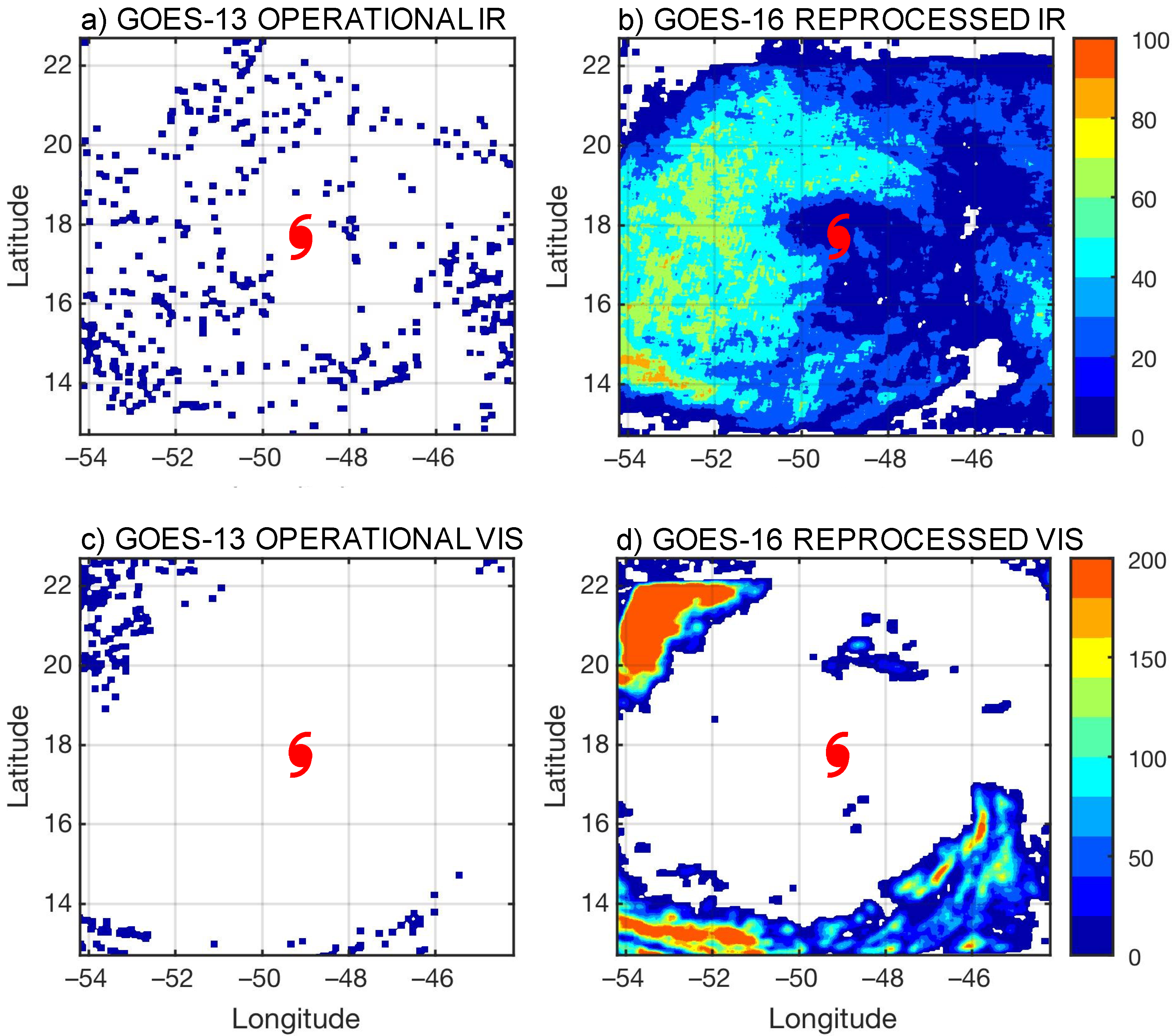
The enhanced AMV datasets using the modified reprocessing strategies were created at 15-min intervals from four GOES-16 ABI bands: visible (VIS, Channel 2, local daytime only), IR shortwave (SWIR, Channel 7, local nighttime only), IR water vapor cloud top (WVCT, Channel 8) and IR longwave (IR, Channel 14). The AMV derivation algorithm employs a nested tracking technique and is basically the same as used for operational processing at NOAA/NESDIS [24]. As mentioned above, the derived AMVs benefit from the improved temporal sampling of the ABI meso sector, and, importantly, the dataset processing strategy is optimized for enhanced coverage over and around a targeted TC. Given the increased spatiotemporal resolution (including good image navigation/co-registration), the reprocessed AMVs produced using the GOES-16 meso-scans are considered to have accuracies superior to that of their conventional counterparts. Figure 3 shows an example of the typical daylight AMV coverage over an area roughly the size of the HWRF d03 assimilation domain for one cycle (+/−3 h from assimilation time) provided by the tailored processing that includes AMVs derived from the limited-area meso-scan sectors targeting Irma. Additionally, shown for comparison are the routine operational (NESDIS) AMVs derived from GOES-13 that were available for assimilation. The enhanced observation density is especially evident in the upper levels over and around the storm core area. Enhanced coverage was less attainable in the core region at low levels due to the extensive storm cirrus canopy but is still an improvement over the operational AMV product. It is expected that GOES-16/17 1-min sector AMV datasets will become operational at NOAA/NESDIS and made publicly available in real time in the near future. Therefore, it is of particular importance that techniques and strategies for their optimal use in operational hurricane models be developed and refined.
2.4. Experiment Design and Evaluation Metrics
To evaluate the impact of the reprocessed GOES-16 AMVs on HWRF forecasts of Hurricane Irma, we first conducted a baseline cycling experiment (hereafter referred to as BASE) that assimilated the full complement of conventional, airborne (including TDR observations collected by NOAA research aircraft when available), and satellite observations, which included the operationally produced AMVs from GOES-13 but excluded any GOES-16 AMVs. Next, a cycling experiment (hereafter referred to as G16REP) was performed, adding the reprocessed GOES-16 AMV dataset. The differences between G16REP and BASE thus reflect the full impact of the new information contained in the reprocessed GOES-16 dataset and provide an indication of the value added by the addition of increased wind vector information owing to the targeted processing strategy.
Since the reprocessed GOES-16 AMV dataset represents a huge increase in observation density, the potential exists that the observation errors themselves are spatially correlated. Failing to account for potential observation error correlation in the HWRF DA system might tend to degrade the analyses and subsequently limit the positive impact on forecasts as well. Given that the nature of the enhanced AMV observation error correlations is at present poorly understood, we conducted a third experiment (G16REP THIN) which thinned the reprocessed GOES-16 AMVs to a 25 km × 50 hPa mesh. We did so with the expectation that observation error correlations would decrease with increased spatial separation of the observations themselves. The differences between G16REP THIN and G16REP therefore represent the impact of reducing, at least partially, the adverse impact of observation error correlation.
An additional factor to be considered is the quality control process used by GSI to eliminate outlying observations. Currently, at the beginning of each outer loop, GSI applies a gross-error check that excludes observations whose observation-minus-background (OMB) values exceed a specified threshold:
where |y – Hx| is the OMB value, egross is the gross-error parameter, emin and emax are maximum and minimum bound parameters, and eobs is the value of the observation error itself. The HWRF default value of egross = 2.5 was used for the above-mentioned experiments. To test the hypothesis that the default gross-error parameter is rejecting too many reprocessed GOES-16 observations, we conducted a fourth assimilation experiment (GROSS2X) in which we set egross = 5.0. To complete the examination of both the thinning and gross-error impacts, we conducted a fifth experiment (GROSS2X THIN) which used egross = 5.0 and thinned the observations to the same mesh used in G16REP THIN. A summary of the experiments and their respective details and differences is given in Table 1.
|y − Hx| > egross × {max[emin,min(emax,eobs)]},
The impacts of the enhanced AMVs from each of the experiments mentioned above were assessed in terms of selected forecast metrics: (1) mean absolute error (MAE) of the TC forecast positions (expressed in nautical miles, nm), (2) MAE and bias of the TC forecast maximum sustained wind (expressed in knots), and (3) MAE and bias of the TC’s forecast area of associated 34-kt winds (expressed in terms of 104 nm2). We defined the area of 34-kt winds as the ellipse whose area is given as
where r1 is defined as half the sum of the 34-kt wind radii in the northeastern and southwestern quadrant, r1 = (R34ne + R34sw)/2, and r2 is defined as half the sum of the 34-kt wind radii in the northwestern and southeastern quadrants, r2 = (R34nw + R34se)/2.
A34 = π × r1 × r2,
Observed values of tropical cyclone position, intensity, and 34-knot wind radii were obtained from the HURDAT2 Best Track database maintained by the National Hurricane Center [25] and were used in the computation of the metrics defined above.
3. Results
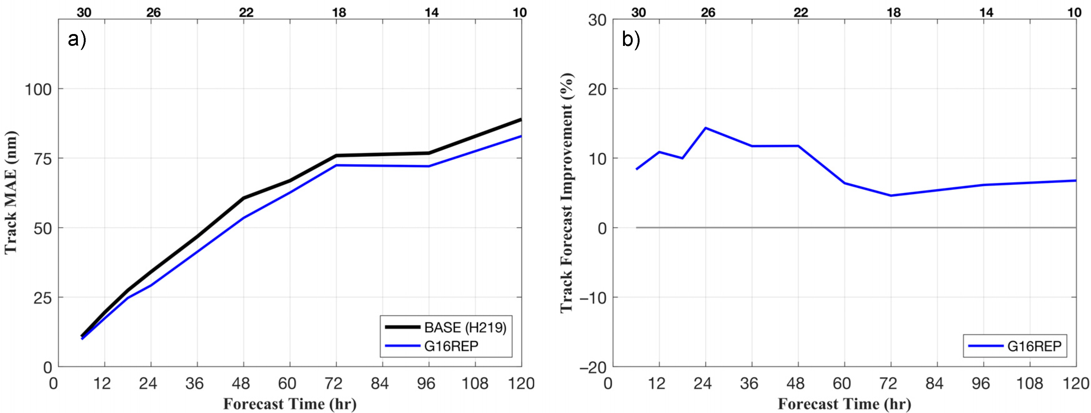
The impact of the reprocessed GOES-16 dataset (G16REP) was first examined relative to the cycling DA experiment that assimilated no GOES-16 AMVs at all (BASE). Relative to BASE, the G16REP reduced the MAE for HWRF track forecasts of Irma at all lead times (Figure 4a), improving upon the BASE track forecasts by 10–15% for lead times out to 48 h (Figure 4b).
The impact on Irma intensity forecasts was somewhat more mixed (Figure 5a). The G16REP experiment yielded small improvements to the MAE for HWRF forecast maximum-sustained wind speed out to 24 h. However, for most lead times after 24 h, the forecast quality was degraded by up to 10% at 72 h (Figure 5b).
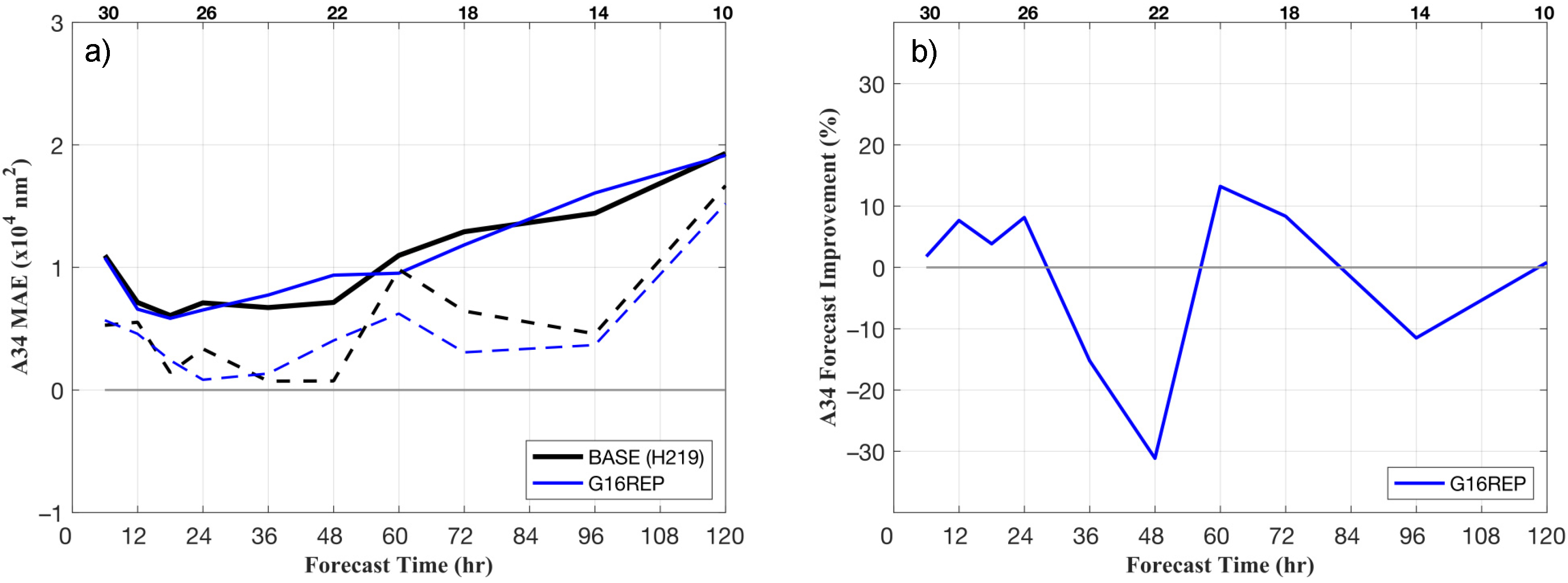
Though track and intensity metrics have traditionally been the gold standard of hurricane forecast evaluation, it is also important to consider storm size, since the areal extent of the TC’s strong wind field defines the envelope of potential impacts (including storm surge). For this metric, we chose the forecast areal extent of 34-kt winds (A34). Figure 6 shows the MAE and % improvement of HWRF forecasts of A34 for the BASE and G16REP experiments. While G16REP slightly improved HWRF forecasts of Irma’s size out to 24 h, as was the case with forecasts of intensity, the impacts beyond 24 h were mixed but more generally less positive.
The DA experiments described above capture the impact of the reprocessed GOES-16 AMV dataset using “out-of-the-box” settings for observation density and quality control in the GSI system. In the next set of experiments, we attempted to better understand how thinning the available data (to alleviate the impact of potential spatial correlation of observation errors) and, conversely, increasing the density of available data (in the case that the pre-tuned quality control in GSI is too strict for the new GOES-16 AMV observations) impact the HWRF forecast results relative to G16REP. Two experiments were conducted, G16REP THIN and GROSS2X, which imposed observation thinning and relaxed quality control on the dataset, respectively, as described in Section 2.4. Additionally, we conducted another experiment, GROSS2X THIN, which examined the impact of both relaxed quality control and observation thinning.
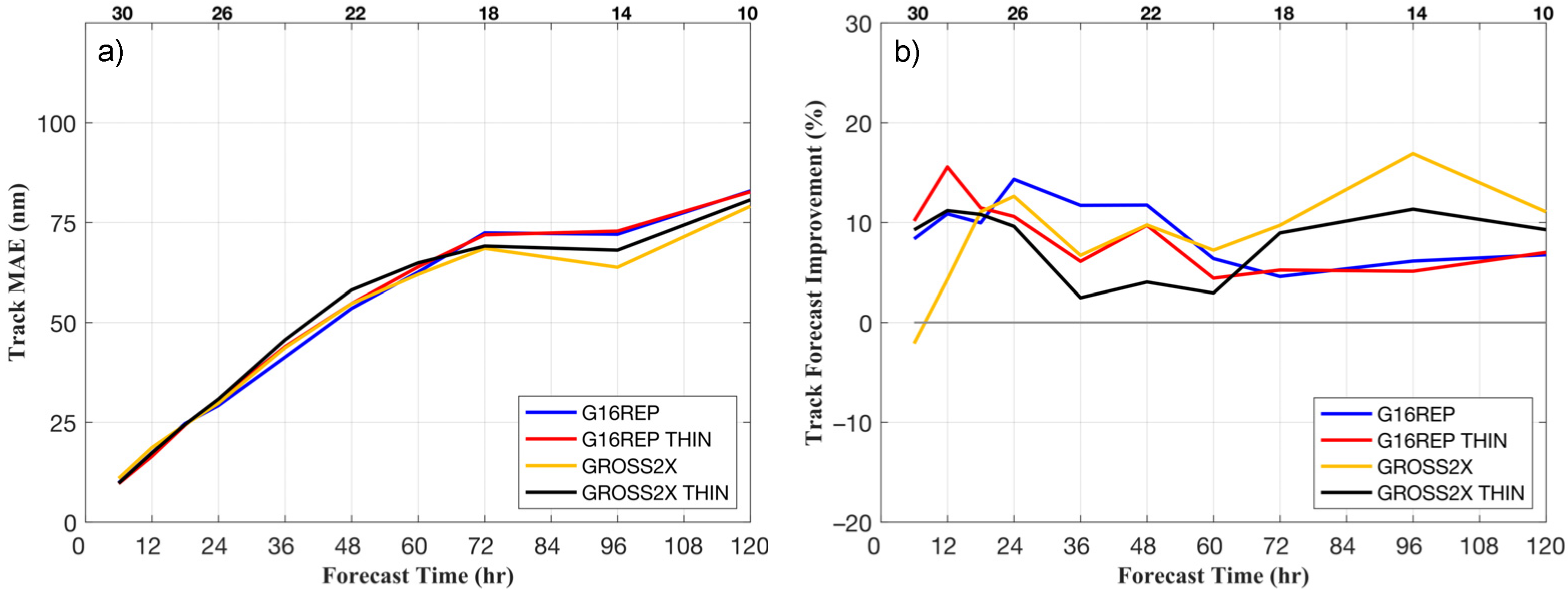
Figure 7a presents the HWRF track forecast results (MAE) for this expanded set of experiments. Each showed a robust improvement over BASE with the exception of GROSS2X, which was slightly worse at 6 h (Figure 7b). With respect to G16REP, observation thinning (G16REP THIN) showed a small positive impact over the first 18 h, but this was negative to neutral beyond that lead time. Relaxing the QC (GROSS2X) resulted in an overall degradation early in the forecast, but notably improved in G16REP beyond 60 h. The combination of the two experiments yielded generally mixed results. In summary, these experiments mainly degraded the G16REP performance out to about 60 h, after which time there was a notable improvement from the relaxation of QC constraints during the assimilation.
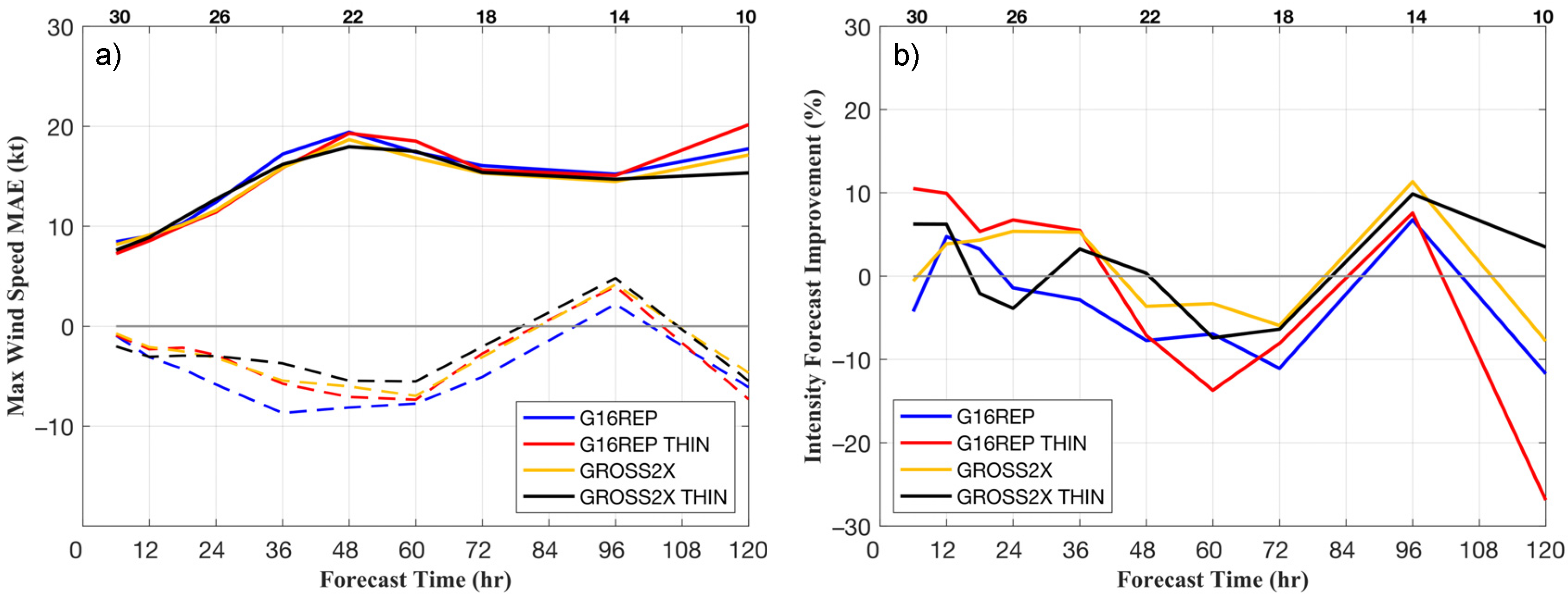
Turning next to HWRF intensity forecast results, both G16REP THIN and GROSS2X showed markedly lower MAE and bias with respect to G16REP for lead times out to 36–48 h (Figure 8a). As with the track forecast impacts (Figure 7b), observation thinning notably helps during the first 12 h of the intensity forecasts relative to BASE (Figure 8b) and continues to have a positive impact on intensity forecasts out to 36 h. The impact beyond about 48 h was mixed with the thinning experiment, but GROSS2X showed small improvements compared to G16REP.
We next considered the effects of observation thinning and relaxed quality control on forecasts of TC size. Figure 9a,b show that for the first 18 h the respective impacts of the two experiments were reversed, with only GROSS2X producing any forecast benefit beyond that offered by the original G16REP configuration, while thinning degraded the forecasts. Beyond that time, the impacts were widely varying and mixed, but the improvements outweighed the degradations with respect to G16REP. Curiously, the GROSS2X THIN experiment MAEs were systematically worse than BASE at all lead times except at 72 h.
Two additional DA experiments were conducted. The first examined the impact of turning off the HWRF vortex initialization (VI) size/intensity adjustment, and the second tested the impact of turning off analysis increment blending in the TC core region (the idea being that this may allow for better cycling of the flow-dependent covariances, which the enhanced AMVs could help control). The forecast impact results of these experiments (not shown) were mixed for Irma’s track, intensity and structure, with no systematic indication of forecast improvement. In this regard, we speculate that 4DEnVAR and hourly cycling (not available yet in the HWRF DA options employed in this study, but coming soon) may be necessary to take full advantage of the vortex-scale information contained in the enhanced AMV observations.
4. Discussion
The intent of this study was to examine the reprocessed GOES-16-enhanced, TC-focused AMV demonstration dataset for Hurricane Irma in terms of HWRF assimilation strategies, in anticipation of these datasets becoming routinely available in the near future. The results presented in Section 3 indicate that the impact of assimilating the reprocessed GOES-16 AMV observations is generally positive with respect to HWRF track forecasts of Hurricane Irma while somewhat mixed for intensity and structure. While the overall sample sizes are too small for results to pass significance tests, the findings can be used to inform and steer future studies that consider much larger samples.
Regarding impacts of the enhanced AMVs on HWRF track forecasts, G16REP produces a robust improvement at all lead times relative to BASE, which assimilates no GOES-16 AMVs. For this case study, DA optimization efforts directed at adjusting the density and quality allowance of the assimilated observations indicate that both thinning of the observations (in this case to a 25 km × 50 hPa mesh in the experiment G16REP THIN) and relaxing of the quality control in GSI via upward adjustment of the gross-error parameter (from 2.5 to 5.0 in experiment GROSS2X) have some promise depending on the forecast lead times.
Impacts on the HWRF intensity forecasts of Irma are mixed. There is evidence that the increased observation density offered by enhanced GOES-16 AMVs improves the initial analyses, which then results in small but positive results early in the forecast period. This was seen in G16REP as well as in the optimization experiments G16REP THIN and GROSS2X. Moreover, G16REP THIN and GROSS2X demonstrated an increased duration of positive impact (from 24 h in the case of G16REP to 48 h in the cases of G16REP THIN and GROSS2X). The experiment which combined thinning and relaxed quality control (GROSS2X THIN) did not distinguish itself from G16REP in terms of intensity impact.
In terms of HWRF forecasts of Irma’s size, the impacts are again mixed; however, the relaxation of GSI quality-control constraints (GROSS2X) does show promise when coupled with adding the enhanced AMVs. In fact, more generally speaking, this case study shows that reducing this constraint produces varying but overall positive impacts resulting from the assimilation of the enhanced AMVs. This suggests the observations deviating from the model background are resolving important dynamical information over the TC core and near environment, as also concluded by [11].
Optimizing the tuning of settings that control observation density and correct for spatial correlation of observation errors with these enhanced GOES-16/17 AMV datasets will be important in achieving optimal forecast performance. As currently configured, the HWRF DA system specifies AMV observation errors as a simple function of pressure altitude. However, the AMV observations themselves come with quality indicators that can be directly used in the pre-assimilation or DA steps as another means towards more effective data selection. Treating the AMV observations errors non-homogeneously in future DA implementations will do much to ensure that the information content of the AMVs is properly projected onto the analysis increments.
It is also important to note that the current HWRF cycling period (i.e., 6 h) is insufficient to fully leverage the increased temporal resolution of the enhanced AMV datasets, which for this study were reprocessed at 15-min intervals. It is conceivable that even more frequently available AMV datasets will become available in the near future from the GOES-16/17 meso scans (i.e., at 5-min. intervals) when the product is operationalized at NOAA/NESDIS. This highlights the importance of model development in the optimal utilization of novel observation sets. Increasing the cycling frequency to hourly (or less) will be an important part of such developmental activities, but continued improvements in model physics, dynamics, and numerics will also be necessary. Each of these aspects of the FV3 and HAFS, currently under development at NWS, NCEP, and EMC, will be crucial in realizing the full potential of the high-density observations of the present and future.
5. Conclusions
In this study, we sought to develop a framework for working towards the optimal use of high-density GOES-16 AMVs in sophisticated, high-resolution NWP and DA systems (here represented by the 2019 version of NCEP’s HWRF model). We demonstrated that the new GOES-16 AMVs have a broadly positive impact on track forecasts for a single high-profile TC case (Irma) from the 2017 Atlantic hurricane season. Although positive forecast impact on Irma’s size and intensity was limited to the first 24 h, we established that, via the imposition of observation thinning and/or relaxation of quality control (thereby allowing more observations to impact the analysis), the period of beneficial intensity forecast impact can be increased. We anticipate that further optimization, with a much larger and more representative set of cases, will lead to more robust results.
However, it must be stressed that optimal utilization of high-density AMVs (as well as other current and future observations types with high density in both space and time) will require upgrades to the model and DA systems as well. More rapid cycling, improved specification of observation errors to include fully non-homogeneous treatment, and even improved model physics will be necessary to extract the maximum benefit from the observations and provide the most accurate and reliable forecasts possible.
Author Contributions
Individual contributions are as follows: conceptualization, C.S.V. and W.E.L.; methodology, W.E.L.; software, W.E.L. and D.S.; validation, W.E.L.; formal analysis, W.E.L. and C.S.V.; investigation, W.E.L. and C.S.V.; resources, C.S.V.; data curation, D.S.; writing—original draft preparation, W.E.L.; writing—review and editing, W.E.L., C.S.V., and D.S.; visualization, W.E.L.; supervision, C.S.V.; project administration, C.S.V.; funding acquisition, C.S.V. All authors have read and agreed to the published version of the manuscript.
Funding
This research was funded by the GOES-R program under element NOAA/NESDIS NA15NES4320001.
Acknowledgments
We wish to thank Jason Sippel of NOAA AOML’s Hurricane Research Division for several fruitful discussions regarding the results of this study. We also extend our thanks to two anonymous reviewers whose comments have improved the manuscript considerably.
Conflicts of Interest
The authors declare no conflict of interest.
References
- Landsea, C.W. Climate Variability of Tropical Cyclones: Past, Present and Future. Storms 2000, 1, 220–241. [Google Scholar]
- Van Oldenborgh, G.J.; Van Der Wiel, K.; Sebastian, A.; Singh, R.; Arrighi, J.; Otto, F.; Haustein, K.; Li, S.; Vecchi, G.; Cullen, H. Attribution of extreme rainfall from Hurricane Harvey. Res. Lett. 2017, 12, 124009. [Google Scholar] [CrossRef]
- Hurricane Weather Research and Forecasting (HWRF) Model: 2018 Scientific Documentation. 2018. Available online: https://dtcenter.org/sites/default/files/community-code/hwrf/docs/scientific_documents/HWRFv4.0a_ScientificDoc.pdf (accessed on 12 April 2019).
- Mehra, A.; Tallapragada, V.; Zhang, Z.; Liu, B.; Zhu, L.; Wang, W.; Kim, H.S. Advancing the State of the Art in Operational Tropical Cyclone Forecasting at NCEP. Trop. Cyclone Res. Rev. 2018, 7, 51–56. [Google Scholar] [CrossRef]
- Velden, C.; Lewis, W.E.; Bresky, W.; Stettner, D.; Daniels, J.; Wanzong, S. Assimilation of high-resolution satellite-derived atmospheric motion vectors: Impact on HWRF forecasts of tropical cyclone track and intensity. Month Weather Rev. 2017, 145, 1107–1125. [Google Scholar] [CrossRef]
- Wu, T.C.; Liu, H.; Majumdar, S.J.; Velden, C.S.; Anderson, J.L. Influence of assimilating satellite-derived atmospheric motion vector observations on numerical analyses and forecasts of tropical cyclone track and intensity. Month Weather Rev. 2014, 142, 49–71. [Google Scholar] [CrossRef] [Green Version]
- Wu, T.C.; Velden, C.S.; Majumdar, S.J.; Liu, H.; Anderson, J.L. Understanding the influence of assimilating subsets of enhanced atmospheric motion vectors on numerical analyses and forecasts of tropical cyclone track and intensity with an ensemble Kalman filter. Month Weather Rev. 2015, 143, 2506–2531. [Google Scholar] [CrossRef]
- Zhang, S.; Pu, Z.; Velden, C.S. Impact of Enhanced Atmospheric Motion Vectors on HWRF Hurricane Analyses and Forecasts with Different Data Assimilation Configurations. Month Weather Rev. 2018, 146, 1549–1569. [Google Scholar] [CrossRef]
- Kim, M.; Kim, H.M.; Kim, J.; Kim, S.M.; Velden, C.; Hoover, B. Effect of Enhanced Satellite-Derived Atmospheric Motion Vectors on Numerical Weather Prediction in East Asia Using an Adjoint-Based Observation Impact Method. Weather Forecast. 2017, 32, 579–594. [Google Scholar] [CrossRef]
- Lim, A.H.N.; Jung, J.A.; Nebuda, S.E. Tropical Cyclone Forecasts Impact Assessment from the Assimilation of HourlyVisible, Shortwave, and Clear-Air Water Vapor Atmospheric MotionVectors in HWRF. Weather Forecast. 2019, 34, 177–198. [Google Scholar] [CrossRef]
- Li, J.; Li, J.; Velden, C.; Wang, P.; Schmit, T.J.; Sippel, J. Impact of rapid-scan-based dynamical information from GOES-16 on HWRF hurricane forecasts. J. Geophys. Res. Atmos. 2020, 125, e2019JD031647. [Google Scholar] [CrossRef]
- Stettner, D.; Velden, C.; Rabin, R.; Wanzong, S.; Daniels, J.; Bresky, W. Development of Enhanced Vortex-Scale Atmospheric Motion Vectors for Hurricane Applications. Remote Sens. 2019, 11, 1981. [Google Scholar] [CrossRef] [Green Version]
- Hurricane WRF (HWRF) Public Download Site Curated by the Developmental Testbed Center. Available online: https://dtcenter.org/community-code/hurricane-wrf-hwrf/download (accessed on 25 June 2020).
- Han, J.; Wang, W.; Kwon, Y.C.; Hong, S.Y.; Tallapragada, V.; Yang, F. Updates in the NCEP GFS cumulus convection schemes with scale and aerosol awareness. Weather Forecast. 2017, 32, 2005–2017. [Google Scholar] [CrossRef]
- Ferrier, B.S.; Jin, Y.; Lin, Y.; Black, T.; Rogers, E.; DiMego, G. Implementation of a New Grid-Scale Cloud and Precipitation Scheme in the NCEP Eta Model. In Proceedings of the 19th AMS Conference on Weather Analysis and Forecasting/15th AMS Conference on Numerical Weather Prediction, San Antonio, TX, USA, 11–16 August 2002. [Google Scholar]
- Aligo, E. The New- Ferrier-Aligo Microphysics in the NCEP 3-km NAM Nest. In Proceedings of the 97th AMS Annual Meeting, Seattle, WA, USA, 21–26 January 2017. [Google Scholar]
- Iacono, M.J.; Delamere, J.S.; Mlawer, E.J.; Shephard, M.W.; Clough, S.A.; Collins, W.D. Radiative forcing by long-lived greenhouse gases: Calculations with the AER radiative transfer models. J. Geophys. Res. 2008, 113, D13103. [Google Scholar] [CrossRef]
- Kwon, Y.C.; Lord, S.; Lapenta, B.; Tallapragada, V.; Liu, Q.; Zhang, Z. Sensitivity of Air-sea Exchange Coefficients (Cd and Ch) on Hurricane Intensity. In Proceedings of the 29th Conf. on Hurricanes and Tropical Meteorology, Tucson, AZ, USA, 9–14 May 2010. [Google Scholar]
- Han, J.; Witek, M.L.; Teixeira, J.; Sun, R.; Pan, H.L.; Fletcher, J.K.; Bretherton, C.S. Implementation in the NCEP GFS of a Hybrid Eddy-Diffusivity Mass-Flux (EDMF) Boundary Layer Parameterization with Dissipative Heating and Modified Stable Boundary Layer Mixing. Weather Forecast. 2016, 31, 341–352. [Google Scholar] [CrossRef]
- Yablonsky, R.M.; Ginis, I.; Thomas, B.; Tallapragada, V.; Sheinin, D.; Bernardet, L. Description and analysis of the ocean component of NOAA’s Operational Hurricane Weather Research and Forecasting Model (HWRF). J. Atmos. Oceanic Technol. 2015, 32, 144–163. [Google Scholar] [CrossRef] [Green Version]
- Environmental Modeling Center (EMC) Gridpoint Statistical Interpolation (GSI) GitHub Site. Available online: https://github.com/NOAA-EMC/GSI (accessed on 11 April 2019).
- NOAA HRD WP-3 Doppler Radar page. Available online: https://www.aoml.noaa.gov/hrd/about_hrd/HRD-P3_radar.html (accessed on 25 June 2020).
- Cangialosi, J.P.; Latto, A.S.; Berg, R. National Hurricane Center Tropical Cyclone Report, Hurricane Irma (AL112017). 2018, NOAA/National Hurricane Center, 111 pp. Available online: https://www.nhc.noaa.gov/data/tcr/AL112017_Irma.pdf (accessed on 11 April 2019).
- Bresky, W.C.; Daniels, J.M.; Bailey, A.A.; Wanzong, S.T. New methods toward minimizing the slow speed bias associated with atmospheric motion vectors. J. Appl. Meteor. Climatol. 2012, 51, 2137–2151. [Google Scholar] [CrossRef]
- Landsea, C.W.; Franklin, J.L. Atlantic Hurricane Database Uncertainty and Presentation of a New Database Format. Month Weather Rev. 2013, 141, 3576–3592. [Google Scholar] [CrossRef]
Figure 1.
Track of Hurricane Irma (2017) from its formation west of the Cape Verde Islands on 30 August to its dissipation over the southeastern United States on 12 September. Filled circles indicate the position of Irma at 00 UTC of the day indicated. The dashed portions of Irma’s track reflect those time periods during which cycling data assimilation was not performed.

Figure 2.
Intensity (maximum sustained winds, kt) time series of hurricane Irma (2017) from its formation west of the Cape Verde Islands on 30 August until its dissipation over the southeastern United States on 12 September. The dashed portions of the time series reflect those time periods for which cycling data assimilation was not performed.

Figure 3.
Illustration of AMV observation density available for assimilation into HWRF for one analysis cycle during the Hurricane Irma (2017) case study. The top row depicts the total number of IR-channel AMVs contained in the 100–300 hPa layer, summed over 10 km × 10 km grid boxes, derived from (a) GOES-13 operational, and (b) GOES-16 reprocessed using 1-min ABI imagery. The bottom row depicts the total number of VIS-channel AMVs contained in the 700–1000 hPa layer derived from (c) GOES-13 operational, and (d) GOES-16 reprocessed using 1-min ABI imagery. The red hurricane symbol indicates the center of Irma at the analysis time.

Figure 4.
Hurricane Irma (2017) HWRF track forecast MAE (nm) verified against NHC Best Track for BASE (heavy black line) and G16REP (blue line) in (a). Percentage improvement in MAE relative to BASE is shown in (b). The number of verifying forecasts for each lead time is shown in black across the top of each plot.

Figure 5.
Hurricane Irma (2017) HWRF intensity (maximum wind speed, kt) forecast MAE (solid) and bias (dashed) verified against NHC Best Track for BASE (heavy black line) and G16REP (blue line) in (a). Percentage improvement in MAE relative to BASE is shown in (b). The number of verifying forecasts for each lead time is shown in black across the top of each plot.

Figure 6.
Hurricane Irma (2017) HWRF areal extent of 34-kt winds (A34) (104 nm2), forecast MAE (solid) and bias (dashed), verified against NHC Best Track for BASE (heavy black line) and G16REP (blue line) in (a). Percentage improvement in MAE relative to BASE is shown in (b). The number of verifying forecasts for each lead time is shown in black across the top of each plot.

Figure 7.
Hurricane Irma (2017) HWRF track forecast MAE (nm) verified against NHC Best Track for G16REP (blue), G16REP THIN (red), GROSS2X (gold), and GROSS2X THIN (black) in (a). The percentage improvement in MAE relative to BASE is shown in (b). The number of verifying forecasts for each lead time is shown in black across the top of each plot.

Figure 8.
Hurricane Irma (2017) HWRF intensity (maximum wind speed, kt) forecast MAE (solid) and bias (dashed) verified against NHC Best Track for G16REP (blue), G16REP THIN (red), GROSS2X (gold), and GROSS2X THIN (black) in (a). Percentage improvement in MAE relative to BASE is shown in (b). The number of verifying forecasts for each lead time is shown in black across the top of each plot.

Figure 9.
Hurricane Irma (2017) HWRF areal extent of 34-kt winds (A34) (104 nm2) forecast MAE (solid) and bias (dashed) verified against NHC Best Track for G16REP (blue), G16REP THIN (red), GROSS2X (gold), and GROSS2X THIN (black) in (a). Percentage improvement in MAE relative to BASE is shown in (b). The number of verifying forecasts for each lead time is shown in black across the top of each plot.


Table 1.
Configuration of the HWRF GOES-16-enhanced AMV assimilation experiments.
| Experiment | GOES-16 AMV Dataset | AMV Thinning Mesh | AMV Gross-Error Parameter |
|---|---|---|---|
| BASE | none | none | 2.5 |
| G16REP | reprocessed | none | 2.5 |
| G16REP THIN | reprocessed | 25 km × 50 hPa | 2.5 |
| GROSS2X | reprocessed | none | 5.0 |
| GROSS2X THIN | reprocessed | 25 km × 50 hPa | 5.0 |
© 2020 by the authors. Licensee MDPI, Basel, Switzerland. This article is an open access article distributed under the terms and conditions of the Creative Commons Attribution (CC BY) license (http://creativecommons.org/licenses/by/4.0/).
Share and Cite
MDPI and ACS Style
Lewis, W.E.; Velden, C.S.; Stettner, D. Strategies for Assimilating High-Density Atmospheric Motion Vectors into a Regional Tropical Cyclone Forecast Model (HWRF). Atmosphere 2020, 11, 673. https://doi.org/10.3390/atmos11060673
AMA Style
Lewis WE, Velden CS, Stettner D. Strategies for Assimilating High-Density Atmospheric Motion Vectors into a Regional Tropical Cyclone Forecast Model (HWRF). Atmosphere. 2020; 11(6):673. https://doi.org/10.3390/atmos11060673
Chicago/Turabian StyleLewis, William E., Christopher S. Velden, and David Stettner. 2020. "Strategies for Assimilating High-Density Atmospheric Motion Vectors into a Regional Tropical Cyclone Forecast Model (HWRF)" Atmosphere 11, no. 6: 673. https://doi.org/10.3390/atmos11060673
Note that from the first issue of 2016, this journal uses article numbers instead of page numbers. See further details here.