On the Buoyancy Subrange in Stratified Turbulence

Abstract

This study is motivated by the importance of the stratified turbulence in geophysical flows. We present a theoretical analysis of the buoyancy subrange based on the theory of strongly stratified turbulence. Some important turbulent scales and their relations are explored. Scaling constants of the buoyancy subrange scaling laws for both kinetic and potential energy spectra are derived and analyzed. It is found that these constants are functions of the horizontal Froude number $F{r}_h$. For the potential energy spectrum, the scaling constant also depends on the turbulent flux coefficient of $\Gamma$.

1. Introduction

The vertical density stratification and velocity profile characterize the dynamics of our atmosphere. Due to the effects of turbulence, the behavior of such stratified shear flows is highly complex and remains one of the important unresolved problems of classical mechanics. Because of this complexity, a study of geophysical turbulence is essential in many aspects. First of all, these processes play a critical role in determining the mixing and vertical transport of passive tracers. They also contribute to the dissipation of waves and tides in the Mesosphere and Lower Thermosphere region. Second, geophysical turbulence and gravity waves (GWs) are the main sources of uncertainty and bias in Global Circulation Models. Third, many dynamical processes with regards to GWs, such as GW instability, breaking, and nonlinear interaction, contribute to atmospheric turbulence and also are affected by it. A vivid example of such complex dynamics is the summer mesopause, which is nearly 100 K colder than a radiatively controlled state, because of the dynamical effects related to GWs and turbulence [1,2].

Despite its central role in the middle atmosphere, geophysical turbulence is a small-scale phenomenon, which makes high-resolution measurements from the ground or in-situ an intrinsically complicated task to accomplish. The presence of stratification further increases the complexity of mesoscale dynamics. Stratified turbulence that is three-dimensional and vertically anisotropic extends to horizontal scales of ten to hundreds kilometers. Being more persistent than isotropic turbulence, it can non-linearly interact with mesoscale GWs. The spectral region where this non-linear interaction takes place is called the buoyancy subrange.

In the present study, we utilize the theory of stratified turbulence to define buoyancy subrange as a region between buoyancy ($L_b$) and Ozmidov ($L_o$) scales. The existence of this region in geophysical turbulence was confirmed only recently using data from in-situ measurements [3] (see [4] for more information on the rocket experiment). A brief historical review on the buoyancy subrange is presented in Section 2. Some valuable scaling relations are discussed in Section 3. Scaling law constants for the buoyancy subrange are analyzed in Section 4. A short discussion on the possible application of our results is given in Section 5. Conclusions are summarized in Section 6.

2. An Overview of the Spectral Properties in the Buoyancy Subrange

The vertical spectra of horizontal kinetic and potential energy of stratified turbulence despite their simple form express the dynamics that are more complex than the horizontal one. Due to the effect of vertical stratification, that begins to play a role in the atmosphere at several kilometers down to tens of meters vertical scales, there is a buoyancy subrange in these spectra. The first attempts to quantify the effects of stable stratification were performed by Lumley [5] and Shur [6]. Under the assumption that turbulence, suppressed by vertical stratification [7], controls the flow dynamics at certain scales, it was found that the spectrum exhibits a “knee” at the buoyancy scale defined as

$$L_b=\sqrt{ϵ/N^3}.$$

(1)

Here $ϵ$ is the turbulent dissipation rate of kinetic energy, and N is the Brant-Väisälä frequency. In particular, it was found that the vertical spectrum exhibits isotropic $E\left(k\right)\sim {ϵ}^{2/3}{k}_z^{-5/3}$ slope at scales smaller than (1) and should have

$$E\left(k\right)\sim N^2{k}_z^{-3}$$

(2)

spectral dependence at larger scales. Later, the scale (1) was named an Ozmidov scale [8] in the oceanological community, although it was first derived in Dougherty [9], who investigated an anisotropy in the Mesosphere and Lower Thermosphere region. In the present study, we use this standard definition of (1), namely, the Ozmidov scale ($L_o$), as it is commonly accepted in the modern-day stratified turbulence community.

Another important result obtained by Lumley [5] suggests that the spectral flux ${ϵ}_k\left(k_z\right)$ of kinetic energy has the following form

$${ϵ}_k\left(k_z\right)=ϵ{(1+{(k_o/k_z)}^{4/3})}^{3/2},\mathrm{here}ϵ=2\nu {\int }_{k_{\lambda }}^{k_o}{E}_{kin}\left(k_z\right)d{k}_z,$$

(3)

$ϵ$ is the turbulent dissipation rate, which is equivalent to the net spectral flux in inertial subrange, $\nu$ is the kinematic viscosity, $E_{kin}$ is the spectral kinetic energy of the stationary flow, $k_o=\sqrt{N^3/ϵ}$ is the wavenumber of Ozmidov scale, and $k_{\lambda }$ is the wavenumber of Taylor microscale. From (3) follows that not all kinetic energy supplied at large scales $k_z<k_o$ is dissipated at scales $k_z>k_o$ and Lumley proposed that the difference of spectral fluxes should work against gravity.

The first observational confirmation of the (2) was reported by Gregg [10]. From the analysis of the vertical temperature probes taken at the North Pacific, they have found that vertical spectrum changes its slope at scales below 10 m from $k_z^{-2}$ to $k_z^{-3}$. It was proposed that either internal GWs that dominate the low-wavenumber part of the energy spectrum change their dynamics or $k_z^{-3}$ is a true fine-scale turbulence spectrum. An alternative hypothesis for the explanation of $k_z^{-3}$ spectral dependence, but this time for the atmosphere, was proposed in Dewan [11] and VanZandt [12]. Here authors hypothesize that the buoyancy subrange can be generated by internal GWs trapped inside the stratified layer (sometimes also called the buoyancy waves). A model for this dynamics was first proposed by Garrett and Munk [13] and later became widely known as a Garrett-Munk spectrum. A slightly different explanation of the (2) was given by Phillips [14], who proposed that internal GWs propagate upwards and grow in height until they become unstable due to shear or convective instabilities [15,16,17,18]. Thus, at the onset of instability, internal GWs exhibit a saturated spectrum with the slope of the form (2). For the mesosphere, the explanation of the buoyancy subrange through the dynamics of saturated GWs was given in Smith et al. [19] (Smith et al. [19], Smith et al. [20]) and for the stratosphere in Dewan and Good [21].

In Weinstock [22], the authors performed a theoretical investigation of the buoyancy flux spectrum in the buoyancy subrange. They pointed out the weakness of the assumption of Lumley [5] that the buoyancy flux spectrum should be dependent on $ϵ$ and $k_z$ only. Thus, having refused the local inertial condition of $ϵ\left(k_z\right)/N^2$ Weinstock [22] found that GWs are strongly damped at wavenumbers $k_z>k_b$, where $k_b$ has the following form

$$k_b=L_b^{-1}=aN/u_h,$$

(4)

here $a=\sqrt{0.8}$ and $u_h$ is the horizontal root-mean-square velocity. At wavenumbers $k_z<k_b$ GWs remain undamped. This result was an important step forward in explanation of the dynamics in buoyancy subrange since Lumley [5]. In the present study, we will follow Weinstock [22] and call $L_b=u_h/N$ the buoyancy lengthscale, which is also a characteristic vertical scale of stratified layer and is different from the outer scale of isotropic turbulence (1) for flows with strong vertical stratification (see Figure 1). Later, Munk [23] suggested that $k_b$ marks the transition between linear (unsaturated) and non-linear (saturated) GWs, while Weinstock [24] analyzed the standard deviation of vertical wind shear and found that the buoyancy subrange of turbulence extends from 50 m to 1000 m in the troposphere and stratosphere.

Finally, it became clear that there are two main hypotheses to explain dynamics in the buoyancy subrange. One approach was that this spectral range is due to saturated GWs [15], which can transport momentum vertically and another that this range is generated by turbulence that is vertically suppressed by stratification [5]. One important parameter that could provide more insight into the $k_z^{-3}$ range phenomenon is the buoyancy flux $B=-\overline{{\rho }^{\prime }g{u}_z}$, which reversibly converts available potential energy into kinetic energy. Although nonlinear wave interactions can redistribute energy, buoyancy flux of integrated wave field is zero. At the same time, turbulence is very efficient in the generation and the downward cascade of buoyancy flux. Thus, analysis of the buoyancy flux could help to determine which of the two above mentioned dynamical concepts dominates the $k_z^{-3}$ spectral range.

According to the Lumley-Richardson approach, spectral flux of kinetic energy in the buoyancy subrange is much larger than $ϵ$: $\Delta ϵ/ϵ\approx {(k_o/k_z)}^2$, here $\Delta ϵ=ϵ\left(k_z\right)-ϵ$. Then buoyancy flux converts $\Delta ϵ$ into the dissipation rate of potential energy ${ϵ}_p\left(k_z\right)={ϵ}_p+\Delta ϵ$. Due to this energy transfer, the ratio $\Gamma ={ϵ}_p/ϵ\approx {(k_o/k_z)}^2\gg 1$. $\Gamma$ is an important parameter called the turbulent flux coefficient. Its realistic order of magnitude is $\Gamma \approx 0.2$, however until now, it is largely unknown how this parameter behaves in the buoyancy subrange [25,26]. So, it suggests that the conclusion of the Lumley-Richardson approach with regards to $\Gamma$ requires some reconsideration. Such correction was proposed by Weinstock [27], who suggested that $\Delta ϵ$ converted into an additional ${ϵ}_p$ is transferred back to larger scales in the buoyancy subrange. Such an inverse cascade of buoyancy flux that converts available potential energy into kinetic is called restratification, and it was indeed found in observational studies [28], numerical simulations of stratified turbulence [29,30,31,32] and simulations of turbulence by gravity wave breaking [33]. An exhaustive review on the restratification phenomenon was written by Gerz and Schumann [34]. Up to some extent, these results could confirm Weinstock’s idea, but two significant circumstances undermine it. The restratification takes place at scales close to $L_o$, where inertial forces become significant [35], and energy transferred to larger scales was typically much smaller than downwards cascaded one. Both issues do not seem to be surmountable, and a new theory that could explain the dynamics of the buoyancy subrange was required.

A different theory that proposes an alternative to the Lumley-Richardson approach explanation was formulated in Holloway [36] (Holloway [36], Holloway [29]). It states that the buoyancy subrange is not dominated by buoyancy flux. Thus, only a small part of kinetic energy is lost by working against gravity, and a unified nonlinear wave interaction theory should be used. Within this approach, GWs and coherent turbulent structures, usually called as pancake-like vortices, are treated as one in the buoyancy subrange. This theory also proposes that spectral fluxes of kinetic and potential energy remain almost unchanged in both buoyancy and inertial subranges.

The approach developed in Holloway [36] (Holloway [36], Holloway [29]) later transformed into the theory of strongly stratified turbulence (SST) formulated in Smyth and Moum [37], Billant and Chomaz [38], Lindborg [39] and Brethouwer et al. [31]. It utilizes two non-dimensional parameters: $F{r}_h=u_h/\left(N{L}_h\right)$ the Froude number and $R{e}_b=ϵ/\left(\nu N^2\right)$ the buoyancy Reynolds number and postulates that SST exists when $F{r}_h\ll 1$ and $R{e}_b\gg 1$. In contrast to the weakly stratified Kelvin-Helmholtz instability regime, in which $F{r}_h\sim 1$, $R{e}_b\gg 1$, generation of the SST regime does not require large-scale wave overturnings. Thus, different dynamic instabilities, such as zigzag instability [38] or Holmboe wave instability [40,41] play crucial roles. However, recently Salehipour et al. [42] and Smyth et al. [43] used an ansatz of Self-Organized Criticality to show that in strongly stratified shear flows turbulence is modulated by Kelvin-Helmholtz instability and has on average $Ri\approx 0.25$ in the whole domain of the flow. That, in turn, suggests that the turbulent flux coefficient should fluctuate around $\Gamma \approx 0.2$. This result supports the hypothesis of Holloway [36] (Holloway [36], Holloway [29]) discussed above, and rejects Equation (3).

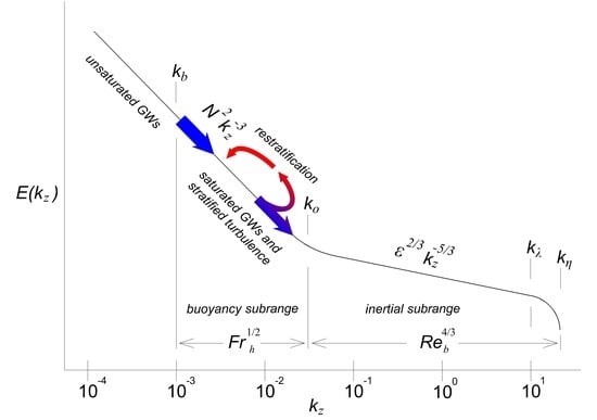
Figure 1 summarizes our knowledge of the buoyancy subrange of the SST regime. It defines locations of the buoyancy and Ozmidov scales. Scaling analysis suggests that $F{r}_h$ controls this subrange, while $R{e}_b$ controls the inertial subrange [44]. Blue arrows represent the constant net spectral energy flux that later continues to cascade down to the smallest scales, and red arrows highlight the region of the spectrum with inverse buoyancy flux. $k_{\lambda }$ is the wavenumber of the Taylor microscale, it is define as

$$\lambda =3.9\sqrt{\nu /N}$$

(5)

(see for more detail Appendix A). Seemingly simplistic form of the inner scale $\lambda$ and its importance for estimation of the turbulent dissipation rate makes (5) of great importance for the geophysical turbulence. An analytic observation that not only $L_o$ but also $\lambda$ is dependent on the local value of the buoyancy frequency N suggests, that even beyond the Ozmidov scale the flow exhibits small-scale vertical anisotropy. Indeed, an analysis of the turbulent velocity strains confirmed the anisotropy that vanishes at high $R{e}_b$ [30,45].

3. On the Concept of Critical Balance

The theory of stratified turbulence proposed by Lindborg [39] suggests that vertical spectra of kinetic and potential energy have the following form

$$\begin{array}{c}\hfill E_k\left(k_z\right)\sim N^2{k}_z^{-3},\end{array}$$

(6)

$$\begin{array}{c}\hfill E_p\left(k_z\right)\sim N^2{k}_z^{-3}.\end{array}$$

(7)

As it is clear from the Introduction, this form of spectra in the buoyancy subrange was quite well studied. However, it was Lindborg [39] who first proposed that stratified turbulence is vertically bounded by $L_b$ and $L_o$ for the largest and the smallest scales, respectively. Recently scaling laws (6), (7) were derived using a concept of critical balance in the theory of wave turbulence [46]. This concept proposes that there is a scale-by-scale balance between GWs and turbulent coherent structures. In other words, it postulates that breaking of gravity wave induces the turbulent eddy with a similar horizontal ($L_h$) and vertical ($L_b$) scales. Using the dispersion relation for incompressible GWs $\omega =N{k}_h/k_z$ and a characteristic turbulent timescale of ${\tau }^{-1}=u_h{k}_h$, here $k_h,u_h$ are the characteristic horizontal length and velocity scales, it is possible to reconstruct the scaling $k_z=N/u_h$ derived by Billant and Chomaz [38]. Then, using a property of horizontal isotropy of the stratified turbulence, it is easy to show that characteristic horizontal velocity satisfies a Kolmogorov-like scaling

$$u_h\sim {ϵ}^{1/3}{k}_h^{-1/3}.$$

(8)

Together with the scaling for buoyancy scale Equation (8) allows obtaining a relation between characteristic horizontal and vertical scales in stratified turbulence

$$L_b=L_o^{2/3}{L}_h^{1/3}.$$

(9)

Here $L_b=u_h/N$ is the buoyancy scale [38], $L_o=\sqrt{ϵ/N^3}$ is the Ozmidov scale [8,9] and $L_h=u_h^3/ϵ$ is the horizontal integral scale [47]. An interesting feature of relation (9) is that it allows us to explicitly define horizontal and vertical scales that contribute to the buoyancy subrange of stratified turbulence. Using a typical numbers for $L_o=100$ m and $L_b=1000$ m for the mesosphere we can find that the largest horizontal scale of the stratified turbulence is $L_h=100$ km. As, $L_h$ is a horizontal outer scale of turbulence it closely correlates with measurements of the spectrum that exhibit change of its form from $k_h^{-3}$ to $k_h^{-5/3}$ [16,48,49,50].

According to the concept of critical balance [46] relation (9) suggests the largest scales of GWs that break in the stably stratified atmospheric flow and contribute to the stratified turbulence. However, GWs of the smaller than horizontal $L_h$ and vertical $L_b$ sizes also contribute to the stratified turbulence even without breaking. For better physical interpretation of the relation (9), it is possible to rewrite it in the following form

$$L_h=F{r}_h^{-1}{L}_b,$$

(10)

where the horizontal Froude number defines the strength of stratification of the flow [44].

4. On Scaling Law Constants in the Buoyancy Subrange

As can be seen from Figure 1, the buoyancy scale is the largest scale of the buoyancy subrange, which spans from $L_b$ to $L_o$, and not of the inertial subrange. With this analytic consideration, let us find scaling constants for (6) and (7). Following the analysis presented in Fukao et al. [51], we may write the following relations for inertial and buoyancy subranges separately

$$\begin{array}{ccc}\hfill \frac{1}{2}\overline{{\left(u_{rms}\right)}^2}& =& {\int }_{k_{\nu }}^{k_o}\alpha {ϵ}^{2/3}{k}_z^{-5/3}d{k}_z,\hfill \end{array}$$

(11)

$$\begin{array}{ccc}\hfill \frac{1}{2}\overline{{\left(u_b^h\right)}^2}& =& {\int }_{k_o}^{k_b}\beta N^2{k}_z^{-3}d{k}_z,\hfill \end{array}$$

(12)

here $\overline{\left(u_{rms}\right)}$ and $\overline{\left(u_b^h\right)}$ are root-mean-square velocities of inertial and buoyancy subranges, respectively, and $\alpha =0.5$ is the Kolmogorov constant for inertial subrange [52], and $\beta$ is the constant for buoyancy subrange. Alternatively, the value of Kolmogorov constant is derived in Appendix B. Due to additional condition of marginally weak stratification of the atmosphere its value is smaller ($\alpha =0.42$) than the classical one.

Integrals (11) and (12) are solved with an assumption that $ϵ$ and N are not functions of vertical wavenumber $k_z$. Thus, the following relations for turbulent dissipation rates are obtained

$$\begin{array}{ccc}\hfill {ϵ}_{in}=C_{1}N\overline{{\left(u_{rms}\right)}^2},& & C_1={\alpha }^{-1}{\left[1-{\left(\frac{k_o}{k_{\nu }}\right)}^{2/3}\right]}^{-1},\hfill \end{array}$$

(13)

$$\begin{array}{ccc}\hfill {ϵ}_b=C_{2}N\overline{{\left(u_b^h\right)}^2},& & C_2={\beta }^{-1}{(F{r}_h^{-1}-1)}^{-1}.\hfill \end{array}$$

(14)

As can be seen, the functional form of turbulence dissipation rate relations in (13) and (14) are similar in both subranges. However, it is necessary to indicate that due to a forward turbulent cascade in the stratified turbulence root-mean-square velocities $\overline{\left(u_{rms}\right)}$ and $\overline{\left(u_b^h\right)}$, characteristic for these regimes, are not equal to each other.

For two limiting cases of SST in the inertial subrange ($R{e}_b\gg 1$) and buoyancy subrange ($F{r}_h\ll 1$), it is possible to simplify $C_1$ and $C_2$ scaling constants. In case of intense isotropic turbulent cascade $k_{\nu }\gg k_o$ so that $C_1={\alpha }^{-1}=2.38$, while for strongly stratified flows we have $k_o\gg k_b$ and $F{r}_h\ll 1$, so that $C_2={\beta }^{-1}F{r}_h$.

Assuming equal net spectral energy fluxes for both subranges Holloway [36] (Holloway [36], Holloway [29])

$${\int }_{k_{\nu }}^{k_o}\frac{d{ϵ}_{k_z}\left(k_z\right)}{d{k}_z}d{k}_z={\int }_{k_o}^{k_b}\frac{d{ϵ}_{k_z}\left(k_z\right)}{d{k}_z}d{k}_z={ϵ}_{in}={ϵ}_b=ϵ,$$

(15)

we can define $\beta$ scaling constant through $\alpha$ and $F{r}_h$, as $\beta =F{r}_h\alpha$. Thus, the vertical spectrum of one-dimensional horizontal kinetic energy has the following form

$$E_k\left(k_z\right)=\alpha ({ϵ}^{2/3}{k}_z^{-5/3}+F{r}_h{N}^2{k}_z^{-3}).$$

(16)

Similar to (16), it is possible to derive the vertical spectrum of available potential energy

$$E_p\left(k_z\right)={\alpha }_o({ϵ}^{-1/3}{ϵ}_p{k}_z^{-5/3}+\Gamma F{r}_h{N}^2{k}_z^{-3}),$$

(17)

here ${\alpha }_o=0.68$ is the Obukhov-Corrsin constant, ${ϵ}_p$ is the potential energy dissipation rate, and $\Gamma ={ϵ}_p/ϵ$ is the turbulent flux coefficient (sometimes also called the mixing efficiency) [25,26].

Equations (16) and (17) indicate that scaling parameters in the buoyancy subrange depend on two non-dimensional ratios, namely, the Froude number $F{r}_h$ and the turbulent flux coefficient $\Gamma$.

5. An Implication to Turbulence Strength Measurements Using Radar

A strong correlation between the turbulent kinetic energy dissipation rate and vertical rms velocity fluctuations $ϵ$∼$w_{rms}^3$ is widely used in studies of geophysical turbulence. However, in Weinstock [53], it was shown that a more accurate relation between $ϵ$ and $w_{rms}$ exists for the stably stratified atmosphere. It was demonstrated, that at low vertical velocity fluctuations, typically when $0\le w_{rms}\le 200$ cm s${}^{-1}$, the following relation is more accurate

$$ϵ=0.4w_{rms}^{2}N.$$

(18)

In Hocking [54], it was proposed that turbulent dissipation rates can be calculated from radar measurements of vertical velocity fluctuation. When radar volume is smaller than the largest scales of turbulence than the following relation is valid

$$ϵ=0.47w_{rms}^{2}N.$$

(19)

Otherwise, a more generalized form of this equation shall be used

$$ϵ=0.47c_f^{-2/3}{w}_{rms}^{2}N,$$

(20)

where $c_f$ is a scaling factor, that varies between 0.9 and 2. According to [55] Equation (20) is used when gravity waves significantly contribute to the measured vertical oscillations.

Recent results from the ShUREX campaign [56,57,58] question applicably of (19) and (20) in the troposphere region. It is shown that $ϵ=w_{rms}^3/L_c$ where $L_c\approx$ 50–70 m correlates much better than (19) or (20) with the in-situ measurements for both convective and stratified turbulent conditions. The authors suggest that the characteristic scale $L_c$ is not necessarily related to an effective outer scale of turbulence (the Ozmidov scale $L_o=\sqrt{ϵ/N^3}$) as it is relevant for all cases. However, since it is obtained from the horizontal in-situ turbulence measurements, that are isotropic for both stratified and convective cases, it is highly likely that this scale is still related to the outer scale of turbulence.

Present analysis with the usage of the theory of SST allows us to refine the relation (19). The value $\alpha =0.42$ derived in Appendix B for weakly stratified flow as well as the classical value of the Kolmogorov constant $\alpha =0.5$ are both very close to the one used in (19). In the case of weak-to-strong stratification, it can be shown that

$$\begin{array}{c}\hfill u_b^v=\sqrt{F{r}_h}{u}_{rms},\end{array}$$

(21)

$$\begin{array}{c}\hfill u_{rms}=\sqrt{F{r}_h}{u}_b^h,\end{array}$$

(22)

where $u_b^v$ and $u_b^h$ are the vertical and horizontal rms velocities in the buoyancy subrange and $u_{rms}$ is the rms velocity in the inertial subrange ($u_{rms}=w_{rms}$). Thus, when the corresponding range resolution is larger than the outer scale of turbulence and depending on the measured velocity component, the following relations can be used

$$\begin{array}{cc}\hfill ϵ=0.42F{r}_h{\left(u_b^h\right)}^{2}N,& \mathrm{for}\mathrm{horizontal}\mathrm{velocity}\mathrm{measurements}\hfill \end{array}$$

(23)

$$\begin{array}{cc}\hfill ϵ=0.42F{r}_h^{-1}{\left(u_b^v\right)}^{2}N.& \mathrm{for}\mathrm{vertical}\mathrm{velocity}\mathrm{measurements}\hfill \end{array}$$

(24)

Relation (24) partially correlates with (20) in parameter space. However, that does not necessarily mean that these two relations have a similar physical interpretation. Further analyses are required to settle this issue.

6. Conclusions

The main goal of the present study is to analyze the complexity of dynamics in the buoyancy subrange, which involves GWs and stratified coherent structures, called pancake-like vortices. The results of the present study could be relevant for the remote and in-situ measurements, improvement of the sub-grid scale parameterization schemes, and also for the analysis of uncertainties in future climate projections [59,60].

Following Nazarenko and Schekochihin [46], we have shown that wave turbulence theory supports $k_z^{-3}$ scaling for this subrange and imposes certain constraints on the scales of breaking GWs. These constraints suggest the location of the knee in horizontal energy spectra at $\mathcal{O}$(100–300) km scales. This estimate is following the transition point in the horizontal energy spectrum observed in the stratosphere [48] and also with some other measurements in the mesosphere [16,50] and numerical simulations [49].

An analysis of the scaling constants of the vertical energy spectra in the buoyancy subrange performed in Section 4 has revealed that relations for turbulence dissipation rates in inertial and buoyancy subranges have a similar functional form (see Equations (13) and (14)). For the first time, it was also shown that scaling constants $C_1$ and $C_2$ are both functions of the Froude number.

In Sukoriansky and Galperin [61], using the theory of Quasi-Normal Scale Elimination in the limit of weak stratification, it was shown that the value of the scaling constant is $\beta =0.214$. Our analysis supports this result, although the present study is focused on the strongly stratified turbulent regime.

For the potential energy spectrum, it was found that the turbulent flux coefficient $\Gamma$ is also a part of the scaling constant, it is following the results of Sukoriansky and Galperin [61].

References

- Lindzen, R.S. Turbulence and stress owing to grawity wave and tidal breakdown. J. Geophys. Res. 1981, 86, 9707–9714. [Google Scholar] [CrossRef] [Green Version]
- Lübken, F.J. Thermal structure of the Arctic summer mesosphere. J. Geophys. Res. 1999, 104, 9135–9149. [Google Scholar]
- Avsarkisov, V.; Strelnikov, B.; Becker, E. Analysis of the vertical spectra of density fluctuation variance in the strongly stratified turbuelence. In Proceedings of the 11th International Symposium on Turbulence and Shear Flow Phenomena (TSFP11), Osaka, Japan, 30 July–2 August 2019; pp. 1–5. [Google Scholar]
- Strelnikov, B.; Eberhart, M.; Staszak, T.; Asmus, H.; Strelnikova, I.; Grygalashvyly, M.; Lübken, F.J.; Latteck, R.; Baumgarten, G.; Höffner, J.; et al. Simultaneous in situ measurements of small-scale structures in neutral, plasma, and atomic oxygen densities during WADIS sounding rocket project. Atmos. Chem. Phys. 2019, 19, 114-43-60. [Google Scholar] [CrossRef] [Green Version]
- Lumley, J.L. The spectrum of nearly inertial turbulence in a stably stratified fluid. J. Atmos. Sci. 1964, 21, 99–102. [Google Scholar] [CrossRef]
- Shur, G.H. Experimental studies of the energy spectrum of atmospheric turbulence. Tr. Tsent. Aerolog. Observ. 1962, 43, 79–90. [Google Scholar]
- Richardson, L.F. The supply of energy from and to atmospheric eddies. Proc. R. Soc. 1920, 97, 354–373. [Google Scholar]
- Ozmidov, R.V. On the turbulent exchange in a stably stratified ocean. Izv. Akad. Nauk. SSSR Atmos. Oceanic Phys. Ser. 1 1965, 853, 1950–1954. [Google Scholar]
- Dougherty, J.P. The anisotropy of turbulence at the meteor level. J. atmos. terr. Phys. 1961, 21, 210–213. [Google Scholar] [CrossRef]
- Gregg, M.C. A Comparison of Finestructure Spectra from the Main Thermocline. J. Phys. Oceanogr. 1977, 7, 33–40. [Google Scholar] [CrossRef] [Green Version]
- Dewan, E.M. Stratospheric Wave Spectra Resembling Turbulence. Science 1979, 204, 832–835. [Google Scholar] [CrossRef]
- VanZandt, T.E. A universal spectrum of buoyancy waves in the atmosphere. J. Atmos. Sci. 1982, 9, 575–578. [Google Scholar] [CrossRef]
- Garrett, C.; Munk, W. Space-time scales of internal waves. Geophys. Fluid Dyn. 1972, 2, 225–268. [Google Scholar] [CrossRef]
- Phillips, O.M. The Dynamics of the Upper Ocean; Cambridge University Press: Cambridge, UK, 1977. [Google Scholar]
- Fritts, D.C. Gravity wave saturation in the middle atmosphere: A review of theory and observations. Rev. Geophys. 1984, 22, 275–308. [Google Scholar] [CrossRef]
- Cai, X.; Yuan, T.; Zhao, Y.; Pautet, P.D.; Taylor, M.J.; Pendleton, W.R., Jr. A coordinated investigation of the gravity wave reaking and the associated dynamical instability by a Na lidar and an Advanced Mesosphere Temperature Mapper over Logan, UT (41.7∘ N, 111.8∘ W). J. Geophys. Res. Space Phys. 2014, 119, 6852–6864. [Google Scholar] [CrossRef]
- Yuan, T.; Heale, C.J.; Snively, J.B.; Cai, X.; Pautet, P.D.; Fish, C.; Zhao, Y.; Taylor, M.J.; Pendleton, W.R., Jr.; Wickwar, V.; et al. Evidence of dispersion and refraction of a spectrally broad gravity wave packet in the mesopause region observed by the Na lidar and Mesospheric Temperature Mapper above Logan, Utah. J. Geophys. Res. Atmos. 2016, 121, 579–594. [Google Scholar] [CrossRef] [Green Version]
- Chau, J.L.; Urco, J.M.; Avsarkisov, V.; Vierinen, J.P.; Latteck, R.; Hall, C.M.; Tsutsumi, M. Four-Dimensional Quantification of Kelvin-Helmholtz Instabilities in the Polar Summer Mesosphere Using Volumetric Radar Imaging. Geophys. Res. Lett. 2020, 47, e2019GL086081. [Google Scholar] [CrossRef] [Green Version]
- Smith, S.A.; Fritts, D.C.; VanZandt, T.E. Comparison of mesospheric wind spectra with a gravity wave model. Radio Sci. 1985, 20, 1331–1338. [Google Scholar] [CrossRef]
- Smith, S.A.; Fritts, D.C.; Zandt, T.E.V. Evidence for a saturated spectrum of atmospheric gravity waves. J. Atmos. Sci. 1987, 44, 1404–1410. [Google Scholar] [CrossRef]
- Dewan, E.M.; Good, R.E. Saturation and the “universal” spectrum for vertical profiles of horizontal scalar winds in the atmosphere. J. Geophys. Res.: Atmos. 1986, 91, 2742–2748. [Google Scholar] [CrossRef]
- Weinstock, J. On the theory of turbulence in the buoyancy subrange of stably stratified flows. J. Atmos. Sci. 1978, 35, 634–649. [Google Scholar] [CrossRef] [Green Version]
- Munk, W. Internal waves and small-scale processes. In Evolution of Physical Oceanography; Warren, B.A., Wunsch, C., Eds.; MIT Press: Cambridge, MA, USA, 1981; pp. 264–291. [Google Scholar]
- Weinstock, J. Vertical wind shears, turbulence and non-turbulence in the troposphere and stratosphere. Geophys. Res. Lett. 1980, 7, 749–752. [Google Scholar] [CrossRef]
- Osborn, T.R. Estimates of the local rate of vertical diffusion from dissipation measurements. J. Phys. Oceanogr. 1980, 10, 83–89. [Google Scholar] [CrossRef] [Green Version]
- Maffioli, A.; Brethouwer, G.; Lindborg, E. Mixing efficiency in stratified turbulence. J. Fluid Mech. 2016, 794, R3. [Google Scholar] [CrossRef] [Green Version]
- Weinstock, J. On the theory of temperature spectra in a stably stratified fluid. J. Phys. Oceanogr. 1985, 15, 475–477. [Google Scholar] [CrossRef]
- Dalaudier, F.; Sidi, C. Evidence and interpretation of a spectral gap in the turbulent atmospheric temperature spectra. J. Atmos. Sci. 1987, 44, 3121–3126. [Google Scholar] [CrossRef] [Green Version]
- Holloway, G. The buoyancy flux from internal gravity wave breaking. Dyn. Atmos. Oceans 1988, 12, 107–125. [Google Scholar] [CrossRef]
- Riley, J.J.; Metcalfe, R.W.; Weissman, M.A. Direct numerical simulations of homogeneous turbulence in density-stratified fluids. AIP Conf. Proc. 1981, 76, 79–112. [Google Scholar] [CrossRef]
- Brethouwer, G.; Billant, P.; Lindborg, E.; Chomaz, J.M. Scaling analysis and simulation of strongly stratified turbulent flows. J. Fluid Mech. 2007, 585, 343–368. [Google Scholar] [CrossRef] [Green Version]
- Waite, M.L. Stratified turbulence at the buoyancy scale. Phys. Fluids 2011, 23, 1–12. [Google Scholar] [CrossRef] [Green Version]
- Bouruet-Aubertot, P.; Sommeria, J.; Staquet, C. Stratified turbulence produced by internal wave breaking: two-dimensional numerical experiments. Dyn. Atmos. Oceans 1996, 23, 357–369. [Google Scholar] [CrossRef]
- Gerz, T.; Schumann, U. A Possible Explanation of Countergradient Fluxes in Homogeneous Turbulence. Theoret. Comput. Fluid Dyn. 1996, 8, 169–181. [Google Scholar] [CrossRef] [Green Version]
- Sidi, C. Wave-turbulence coupling. In Coupling Processes in the Lower and Middle Atmosphere; Thrane, E.W., Blix, T.A., Fritts, D.C., Eds.; Kluwer Academic Publishers: Berlin, Germany, 1993; pp. 291–304. [Google Scholar]
- Holloway, G. A conjecture relating oceanic internal waves and small-scale processes. Atmos. Ocean 1983, 21, 107–122. [Google Scholar] [CrossRef] [Green Version]
- Smyth, W.D.; Moum, J.N. Anisotropy of turbulence in stably stratified mixing layers. Phys. Fluids 2000, 12, 1343–1362. [Google Scholar] [CrossRef] [Green Version]
- Billant, P.; Chomaz, J.M. Self-similarity of strongly stratified inviscid flows. Phys. Fluids 2001, 13, 1645–1651. [Google Scholar] [CrossRef] [Green Version]
- Lindborg, E. The energy cascade in a strongly stratified fluid. J. Fluid Mech. 2006, 550, 207–242. [Google Scholar] [CrossRef]
- Holmboe, J. On the behaviour of symmetric waves in stratified shear layers. Geophys. Publ. 1962, 24, 67–113. [Google Scholar]
- Browand, F.K.; Winant, C.D. Laboratory observations of shear-layer instability in a stratified fluid. Bound.-Layer Meteor. 1973, 5, 67–77. [Google Scholar] [CrossRef]
- Salehipour, H.; Peltier, W.R.; Caulfield, C.P. Self-organized criticality of turbulence in strongly stratified mixing layers. J. Fluid Mech. 2018, 856, 228–256. [Google Scholar] [CrossRef] [Green Version]
- Smyth, W.D.; Nash, J.D.; Moum, J.N. Self-organized criticalityin geophysical turbulence. Sci. Rep. 2019, 9. [Google Scholar] [CrossRef] [Green Version]
- Mater, B.D.; Venayagamoorthy, S.K. A unifying framework for parameterizing stably stratified shear-flow turbulence. Phys. Fluids 2014, 26, 036601-1-18. [Google Scholar] [CrossRef]
- Yamazaki, H.; Osborn, T. Dissipation estimates for stratified turbulence. J. Geophys. Res. 1990, 95, 9739–9744. [Google Scholar] [CrossRef]
- Nazarenko, S.V.; Schekochihin, A.A. Critical balance in megnetohydrodynamic, rotating and stratified turbulence: towards a universal scaling conjecture. J. Fluid Mech. 2011, 677, 134–153. [Google Scholar] [CrossRef] [Green Version]
- Davidson, P.A. Turbulence in Rotating, Stratified and Electrically Conducting Fluids; Cambridge University Press: Cambridge, UK, 2013. [Google Scholar]
- Nastrom, G.D.; Gage, K.S. A climatology of atmospheric wavenumber spectra of wind and temperature observed by commercial aircraft. J. Atmos. Sci. 1985, 42, 950–960. [Google Scholar] [CrossRef] [Green Version]
- Liu, H.L. Quantifying gravity wave forcing using scale invariance. Nature Comm. 2019, 10, 1–12. [Google Scholar] [CrossRef] [Green Version]
- Vierinen, J.; Chau, J.L.; Charuvil, H.; Urco, J.M.; Clahsen, M.; Avsarkisov, V.; Marino, R.; Volz, R. Observing Mesospheric Turbulence With Specular Meteor Radars: A Novel Method for Estimating Second-Order Statistics of Wind Velocity. Earth Space Sci. 2019, 6, 1171–1195. [Google Scholar] [CrossRef] [Green Version]
- Fukao, S.; Yamanaka, M.D.; Ao, N.; Hocking, W.K.; Sato, T.; Yamamoto, M.; Nakamura, T.; Tsuda, T.; Kato, S. Seasonal variability of vertical eddy diffusivity in the middle atmosphere 1. Three-year observations by the middle and upper atmosphere radar. J. Geophys. Res. 1994, 99, 18973–18987. [Google Scholar] [CrossRef]
- Sreenivasan, K. On the universality of the Kolmogorov constant. Phys. Fluids 1995, 7, 2778–2784. [Google Scholar] [CrossRef] [Green Version]
- Weinstock, J. Energy dissipation rates of turbulence in a the stable free atmosphere. J. Atmos. Sci. 1981, 38, 880–883. [Google Scholar] [CrossRef] [Green Version]
- Hocking, W.K. The dynamical parameters of turbulence theory as they apply to middle atmosphere studies. Earth Planets Space 1999, 51, 525–541. [Google Scholar] [CrossRef] [Green Version]
- Hocking, W.K.; Roettger, J.; Palmer, R.D.; Sato, T.; Chilson, P.B. Atmospheric Radar; Cambridge University Press: Cambridge, UK, 2016. [Google Scholar]
- Kantha, L.; Luce, H.; Hashiguchi, H. Shigaraki UAV-radar experiment (ShUREX): overview of the campaign with some preliminary results. Earth Planets Space 2017, 4, 1–26. [Google Scholar] [CrossRef] [Green Version]
- Luce, H.; Kantha, L.; Hashiguchi, H.; Lawrence, D.; Doddi, A. Turbulence kinetic energy dissipation rates estimated from concurrent UAV and MU radar measurements. Earth Planets Space 2018, 70, 1–19. [Google Scholar] [CrossRef]
- Kantha, L.; Luce, H.; Hashiguchi, H. On a numerical model for extracting TKE dissipation rate from very high frequency (VHF) radar spectral width. Earth Planets Space 2018, 70, 1–18. [Google Scholar] [CrossRef] [Green Version]
- Dauxois, T.; Peacock, T.; Bauer, P.; Caulfield, C.P.; Cenedese, C.; Gorlé, C.; Haller, G.; Ivey, G.N.; Linden, P.F.; Meiburg, E.; et al. Confronting Grand Challenges in Environmental Fluid Dynamics. arXiv 2019, arXiv:1911.09541. [Google Scholar]
- Caccamo, M.T.; Magazú, S. A physical-mathematical approach to climate change effects through stochastic resonance. Climate 2019, 7, 1–16. [Google Scholar] [CrossRef] [Green Version]
- Sukoriansky, S.; Galperin, B. An analytical theory of the buoyancya-Kolmogorov subrange transition in turbulent flows with stable stratification. Phil. Trans. R. Soc. A 2013, 371, 20120212. [Google Scholar] [CrossRef] [PubMed] [Green Version]
- Tennekes, H.; Lumley, J.L. A First Course in Turbulence; The MIT Press: Berlin, Germany, 1972. [Google Scholar]
- Pope, S.B. Turbulent Flows; Cambridge University Press: New York, NY, USA, 2000. [Google Scholar]
Figure 1.
Schematics of vertical wavenumber spectra of turbulent energy. is the buoyancy scale (4); is the Ozmidov scale (1); is the Taylor microscale (5) and is the Kolmogorov scale. The blue arrows show the constant spectral energy flux and red arrows highlight the region in the buoyancy subrange, where buoyancy flux re-stratifies the flow through partial conversion of potential into kinetic energy.
© 2020 by the author. Licensee MDPI, Basel, Switzerland. This article is an open access article distributed under the terms and conditions of the Creative Commons Attribution (CC BY) license (http://creativecommons.org/licenses/by/4.0/).
Share and Cite
MDPI and ACS Style
Avsarkisov, V. On the Buoyancy Subrange in Stratified Turbulence. Atmosphere 2020, 11, 659. https://doi.org/10.3390/atmos11060659
AMA Style
Avsarkisov V. On the Buoyancy Subrange in Stratified Turbulence. Atmosphere. 2020; 11(6):659. https://doi.org/10.3390/atmos11060659
Chicago/Turabian StyleAvsarkisov, Victor. 2020. "On the Buoyancy Subrange in Stratified Turbulence" Atmosphere 11, no. 6: 659. https://doi.org/10.3390/atmos11060659
Note that from the first issue of 2016, this journal uses article numbers instead of page numbers. See further details here.