Urban CO2 Budget: Spatial and Seasonal Variability of CO2 Emissions in Krakow, Poland


1
Institute of Meteorology and Water Management, National Research Institute, 30-215 Krakow, Poland
2
Faculty of Physics and Applied Computer Science, AGH University of Science and Technology, 30-059 Krakow, Poland
*
Author to whom correspondence should be addressed.
Atmosphere 2020, 11(6), 629; https://doi.org/10.3390/atmos11060629
Submission received: 11 May 2020
/
Revised: 5 June 2020
/
Accepted: 12 June 2020
/
Published: 14 June 2020
(This article belongs to the Special Issue Greenhouse Gases Monitoring, Inventory, and Modelling Studies in Poland)
Abstract
:Krakow, with an area of 327 km2 and over 750,000 inhabitants, is one of the largest cities in Poland. Within the administrative city borders several anthropogenic CO2 source types are located, including car traffic, household coal and natural gas burning, and industrial emissions. Additionally, the biosphere produces its own, seasonally variable, input to the local atmospheric carbon budget. In order to quantify each of CO2 budget contributions to the local atmosphere, a number of analytical and numerical techniques have been implemented. The seasonal variability of CO2 emission from soils around the city has been directly measured using the chamber method; CO2 net flux from an area containing several source types has been measured with a relaxed eddy accumulation—a variation of the eddy covariance method. Global emissions inventory, as well as local statistical data have been utilized to assess anthropogenic component of the budget. As other cities where CO2 budget was quantified, Krakow proved to be a net source of this greenhouse gas, and the calculated annual mean net flux of CO2 to the atmosphere equal 6.1 kg C m−2 is consistent with previous estimations.
1. Introduction
Depending on the estimation method, urban areas occupy from 0.24% to 2.74% of the Earth’s land surface, the Antarctic and Arctic excluded [1]. This relatively small area is inhabited by more than half of the global population, and is estimated to be a source of over 70% of global anthropogenic carbon dioxide emissions [2]. At the same time, urban areas are considered to be a challenge for climatology and meteorology, mostly due to their highly heterogeneous characteristics varying widely in space and time.
Due to the large number of anthropogenic CO2 emissions, urban atmosphere is characterized by elevated concentrations, as well as modified isotope composition (13C/12C and 14C/12C ratios) of this gas (e.g., [3,4,5]). Carbon dioxide released to the urban atmosphere during fossil fuel combustion originates from one of three basic source types: (i) traffic, (ii) individual households (so-called low emission sources), and (iii) industry and power plants (so-called high emission sources). In densely populated urban areas, the respiration of residents also have to be taken into account in local carbon budget [6,7,8,9].
Urban vegetation assimilates CO2 from the local atmosphere, and transforms it into organic compounds through photosynthesis. The total mass of carbon assimilated annually is called gross primary production (GPP). Organic compounds produced in the process of photosynthesis are partly utilized to build plant tissues, whereas other fractions are transformed back to CO2 through the autotrophic respiration, to obtain energy for cellular metabolic processes. The difference between GPP and autotrophic respiration is called net primary production (NPP).
Biogenic emissions of CO2 originate from two major sources: (i) the autotrophic respiration of vegetation, both above and below ground; and (ii) the decomposition of soil organic matter. Soil respiration intensity is determined by the CO2 production in the soil, along with oxygen uptake from air present in soil pores. The term respiration covers a group of processes of aerobic and anaerobic respiration of plants and soil organisms, and the decomposition of soil organic matter. The produced CO2 is transported to the surface mainly through diffusion, driven by the partial pressure difference of CO2 between soil air and adjoining atmosphere. Root respiration has been shown to be a linear function of the aboveground part of the plant volume [10]. Soil respiration intensity is an exponential function of soil temperature [11]. The exponent specific constant, the so-called Q10 coefficient, is defined as the ratio of respiration intensity at the given temperature, and at the temperature higher by 10 °C. Relatively low Q10 values mean that soil is less sensitive to temperature changes: with the increase of temperature, the respiration intensity—and, thus, the CO2 flux from soil—rises slower than for soil with relatively high Q10. Q10 values have been widely studied for soils across different climatic zones and vary within the range of 1.3–3.3, with a median of around 2.4 [11]. The impact of soil moisture on respiration intensity reveals a certain maximum value, above which the number of air-filled pores is insufficient for the soil microorganisms and roots to draw oxygen efficiently. Additionally, with lower air porosity of the soil, the efficiency of CO2 diffusive transport in the soil is diminished. Therefore, above this threshold value, the flux of soil CO2 to the atmosphere decreases. On the other hand, at low levels of soil moisture, respiration intensity decreases, due to an insufficient amount of water being available for microorganisms and plant roots. Between those two thresholds, respiration intensity increases approximately linearly with the soil water content [12].
In aquatic environment, carbon can be found in various forms such as: (i) dissolved inorganic carbon, including dissolved gaseous CO2 and methane; (ii) dissolved organic carbon; and (iii) particulate organic carbon. The concentration of CO2 in water is modified through the same processes which occur on land: photosynthesis, respiration, and the decomposition of organic matter. In addition, it can be influenced by supply of rainwater that contains low amounts of carbon [13] or the weathering of carbonate minerals [14]. Due to the presence of CO2 sources in river bottom sediments and in the water column, the river usually remains supersaturated with respect to CO2, resulting in positive flux of CO2 from the water body to the atmosphere [15]. The contributions of surface waters to the local carbon balance vary between a few and over a dozen percent of net ecosystem flux to the atmosphere, and depend on latitude and river basin topography [13].
In densely populated urban areas, the respiration of humans is a non-negligible part of the local CO2 budget. An average person produces 0.8 mole of CO2 per hour [6]; more sophisticated human metabolism models estimate 21.4 mole of CO2 per day [7]. The contribution of humans to the local CO2 budget depends strongly on the population density, with town emissions up to two orders of magnitude lower than that of a highly urbanized area [9]. In an extreme case, human respiration may account for up to 38% of total CO2 emissions to the local atmosphere [6]. For mid-latitude, well-developed cities this fraction is estimated to be about 5% [8].
The presented study was aimed at constructing a comprehensive carbon budget for Krakow, the second largest city in Poland.
2. Methods
2.1. Study Site
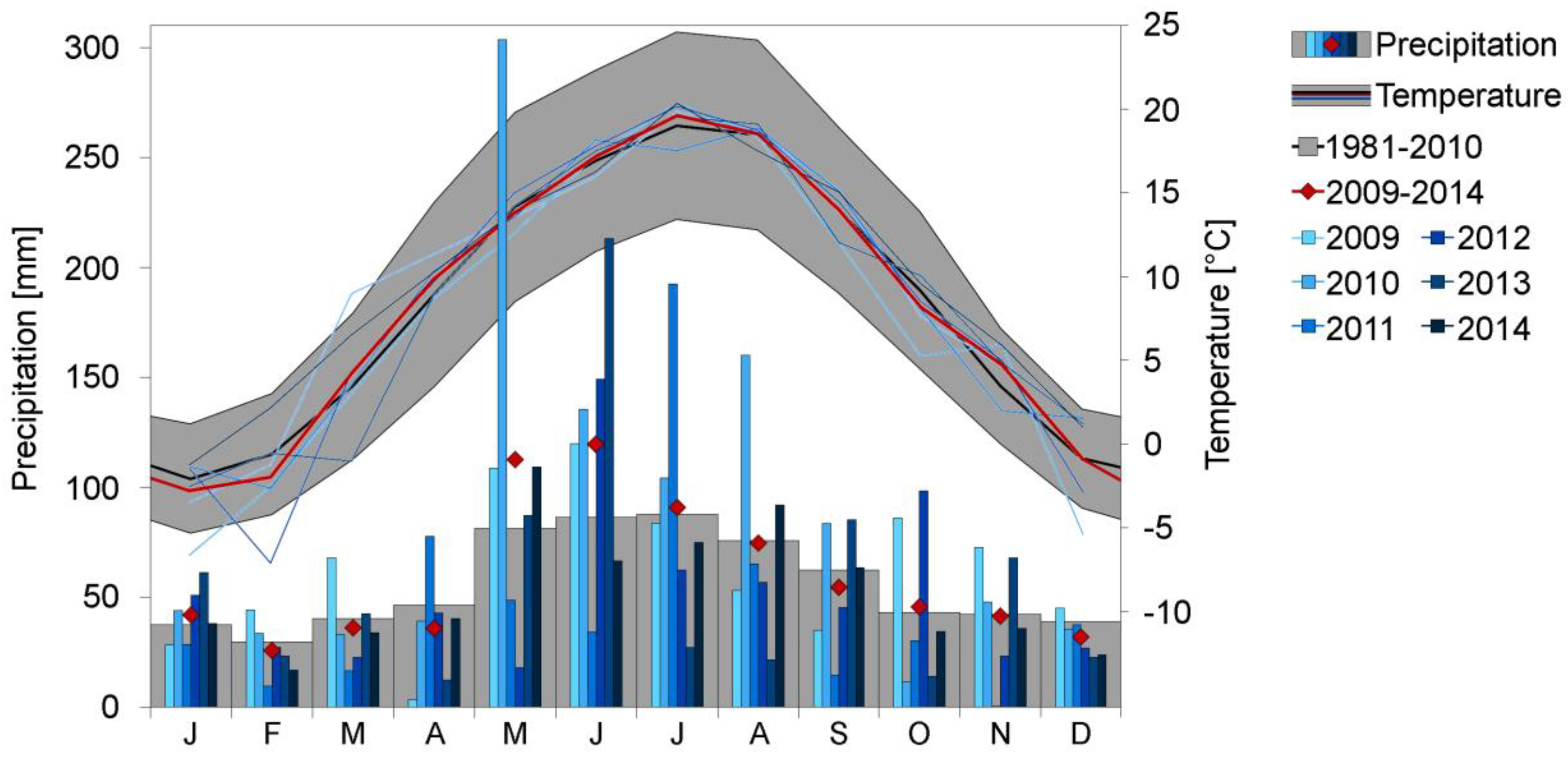
Krakow is located in the southern part of the region called Lesser Poland, in a temperate climate of central Europe. The daily mean temperature is equal to 8.2 °C, with a variation between a minimum of −5.3 °C in January and a maximum of 24.6 °C in July. Precipitation occurs throughout the year with yearly mean amount of 678 mm, with the driest season being winter, with around 30 mm of precipitation per month; the most rain occurs from May to August, with around 80 mm per month on average (calculated for the period 1981–2010; Figure 1). During the study, the monthly mean temperature remained close to the values expected from the city climatology, while warm season precipitation varied significantly over subsequent years (Figure 1).
The city is located in Vistula river valley surrounded by hills. This is the reason of significant wind speed reduction and frequent air temperature inversions. Such conditions stimulate accumulation of CO2 within boundary layer, and result in a high amplitude of the diurnal CO2 concentration cycle (up to 100 ppm), observed especially during winter season [16]. Krakow represents a typical urban environment, with a number of anthropogenic and natural CO2 sources and sinks, like low emission sources, industry, transport, water reservoirs and city biosphere, including citizens and pets. The Vistula flows through Krakow latitudinally. The watercourse length of the Vistula within administrative borders of Krakow is 34 km, compared to the city span of about 26 km. The river is regulated within the city limits, including three navigation dams. Before entering Krakow, the Vistula drains densely populated areas, where agriculture and heavy industry is located. More detailed description of the Vistula river in Krakow reach is available in [17].
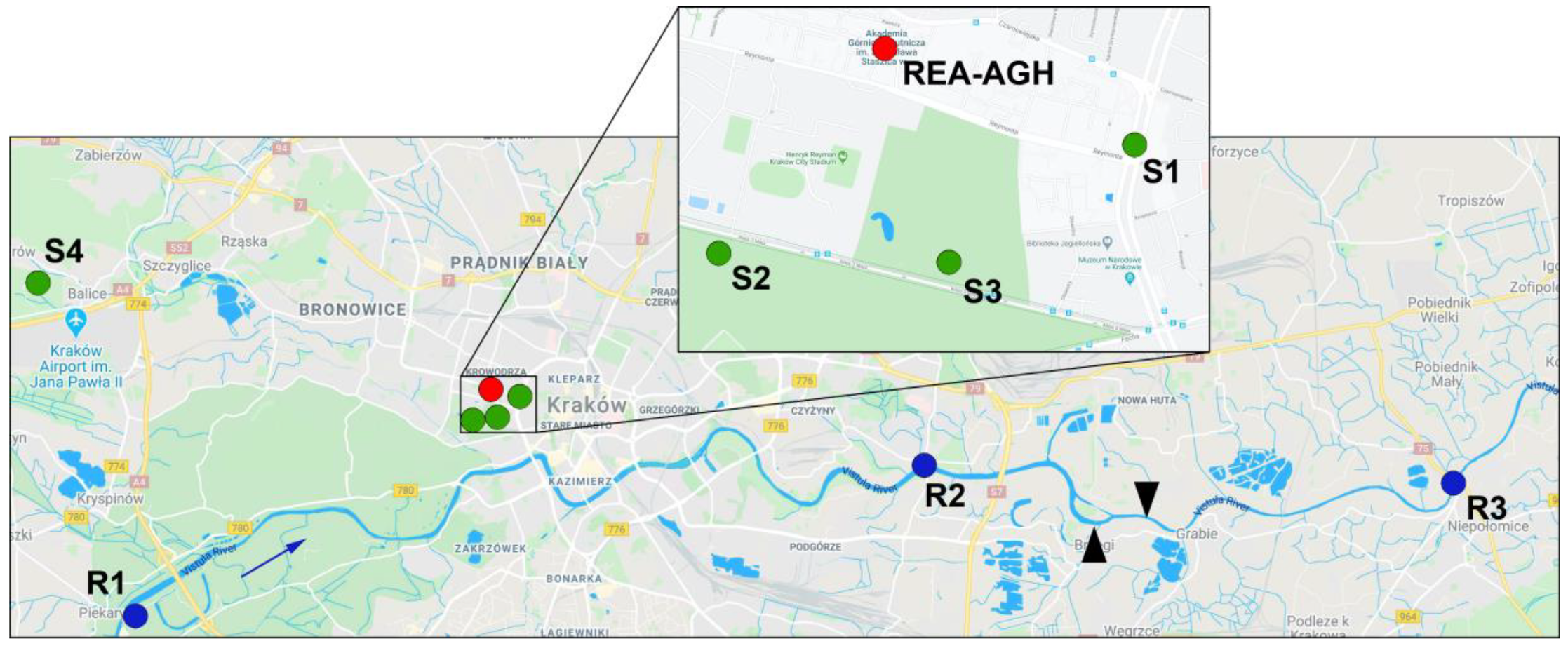
In order to measure CO2 flux from soil, four sites with different type of land cover have been selected across the city (Figure 2). Site S1 was located on a lawn separating two lines of one of the main city traffic arteries. Due to increased emissions from traffic, the local biosphere is exposed to elevated CO2 levels, even 20–40 ppm higher than at other locations in the city. Site S2 was located on the outskirts of a large urban meadow of 48 hectares, which is also a recreational area, and borders low and moderate traffic routes. According to historical records this area has never undergone drastic changes nor an urbanization processes, so the soil at this site has remained undisturbed for at least two hundred years. The measurement sites S1 and S2 have been described in detail in [18]. Site S3 was set up in a park adjacent to the meadow where the S2 site was located. The park was created in the nineteenth century and, since then, has been repeatedly transformed. The measurement site was located on one of the lawns in the least transformed portion of the park, in the vicinity of elm and oak trees. A reference site, S4, was located on a suburban backyard lawn, outside the city administrative boundaries, and far away from busy traffic routes. Soil carbon content at each site has been analyzed with a CNS LECO 2000 elemental analyzer and pH was determined with the potentiometric method. Sites characteristics are presented in Table 1.
Three sites have been selected along the Vistula to measure CO2 flux from the water column: (i) site R1, upon the entrance of the river to the city; (ii) site R2, close to the city center; and (iii) site R3, at the outflow from the city, downstream of the discharge points of municipal wastewater treatment plants (Figure 2). Regular CO2 flux measurements have been performed at those three sites in the course of one year (2011–2012), in approximately monthly time intervals. Apart of CO2 flux, selected physico-chemical parameters of water have been determined (temperature, pH, conductivity, alkalinity) for the calculation of CO2 content in the river. Site characteristics are presented in Table 2.
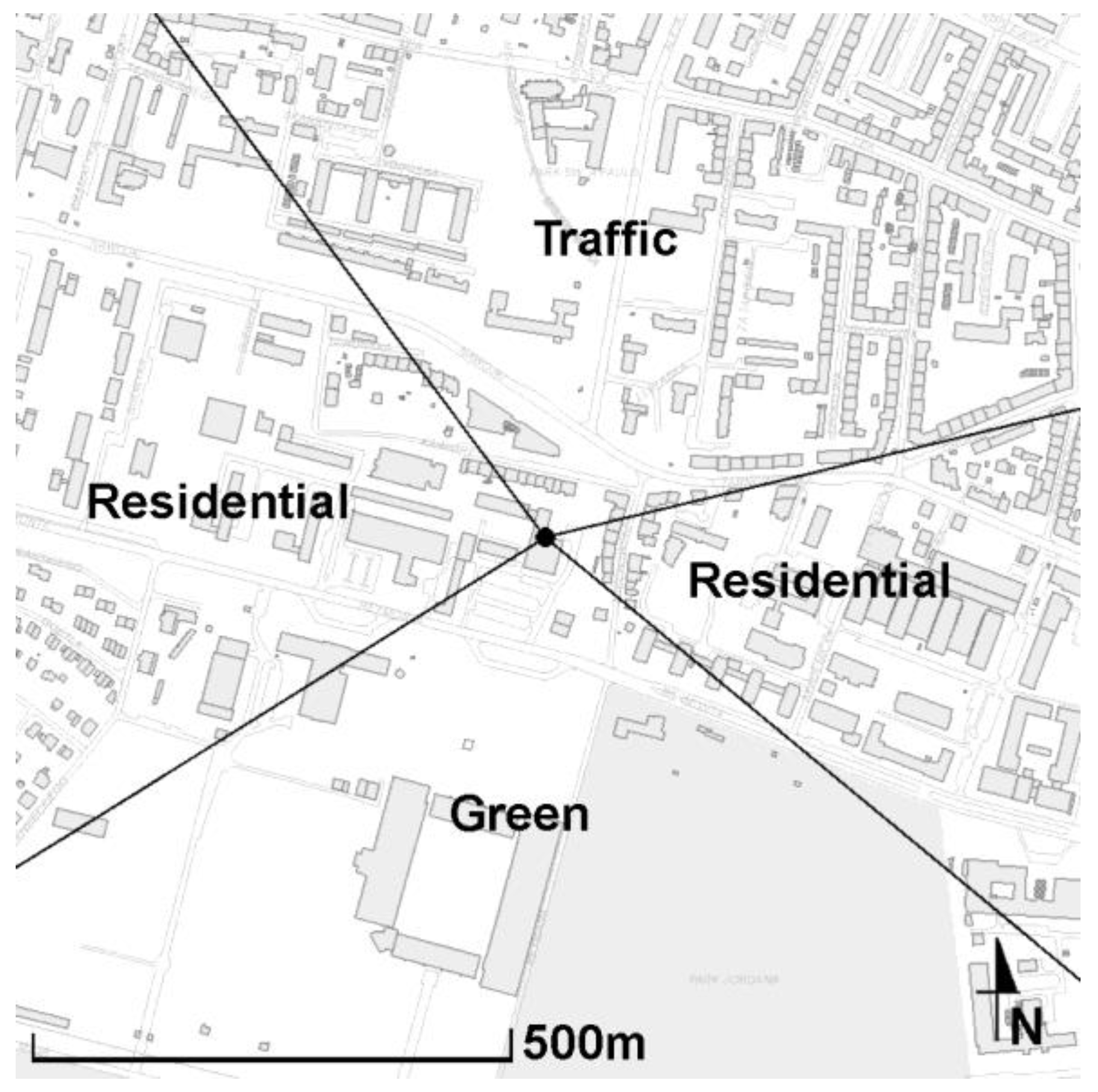
The REA-AGH net CO2 flux measurement site was located within university campus near the city center (Figure 2). Various elements of the urban environment can be identified within 500 m of the site, including traffic routes, built-up areas, and the park, where one of the chamber measurement sites was located. The university campus is located west and east of the site. The area south of the site is mainly green, with the public park and a city stadium, but also with minor traffic routes. North of the site, numerous four- to six-stories household blocks are located. Approximately 115 m north, a busy and often jammed traffic intersection is located. In total, within 500 m of the measurement site, built-up, or otherwise transformed areas comprised 41% of the total area, low-rise green (i.e., lawns) 18%, high-rise green (i.e., trees and bushes) 34%, and roads 6%. Three zones with different prevalent CO2 source type were established according to land use map: (i) traffic zone, located north of the measurement site and including busy traffic routes; (ii) green zone, located south of the site and including several lawns as well as the city park; and (iii) built-up zone, including two separate areas of household and university buildings that are located west and east of the measurement site (Figure 3).
2.2. CO2 Flux Measurements
The CO2 flux from soils and water surfaces within the city limits has been measured directly with chamber method [18,22]. Net CO2 flux from the urban ecosystem was quantified using the relaxed eddy accumulation method [22].
The chamber method has been thoroughly discussed in numerous studies (e.g., [23,24]). Closed (non-steady state) chamber method employed in this study estimates CO2 flux by measuring the rate of change of CO2 concentration within the chamber volume over time. Assuming the air in the chamber headspace to be ideal gas, CO2 flux density F [µmol m−2 s−1] from the area A [m2], which is covered by the chamber is proportional to the rate of CO2 concentration change in the headspace, ∂c/∂t [µmol mol−1 s−1]:
where p stands for atmospheric pressure [Pa]; R is the universal gas constant equal to 8.31 J mol−1 K−1; T–air temperature [K]; V–chamber headspace volume [m3]. As a result of a diffusive character of CO2 emission from the soil or water surface, the increase of CO2 concentration in the headspace volume is best described by exponential function (e.g., [23]).
F = (∂c/∂t) (pV/RTA),
Two different chamber designs have been employed in the study: (i) a stainless steel square-based chamber with the volume of 45 L; and (ii) a cylindrical, stainless steel and plexiglas chamber with a volume of 27 L and a pressure compensation vent [25]. Both chambers have been equipped with stainless steel collars inserted into the ground to avoid leakages. Laboratory and in-situ tests have been performed with both chamber designs. Additionally, a triple-channel system has been designed to simultaneously measure CO2 flux with three identical chambers located on an area within ten-meter radius from the concentration analyzer. The concentration of CO2 in the headspace volume was measured with Vaisala CarboCAP GMP343 probe (Vaisala, Vantaa, Finland) and, starting from 2011, with Picarro G2101i analyzer (Picarro Inc., Santa Clara, California, USA). The initial measurement setup (2009–2011) has been thoroughly discussed in [18].
The chamber measurements of soil CO2 emissions have been performed during a four-year period (2009–2013). Each month, on the same day for all of the sites, a single measurement of the flux was taken. First, chambers collars were pressed into the ground. Unlimited access to the sites meant that it was not possible to leave the collars in the ground, as it is recommended for this type of measurement [23,25]. To compensate for the soil disturbance, chambers were deployed for flux measurement at least fifteen minutes after installing the collar. During this time, the measurement system was vented with ambient air, and the soil temperature and humidity were determined. Soil temperature was measured once around each collar, with a thermocouple probe thermometer at 5 cm depth. When the ground was frozen, the surface air temperature was recorded. Soil humidity was measured at a 5 cm depth three times around each collar with a Theta probe coupled with a Delta T hand-held reader. The collars were newly installed in the ground during each measurement campaign, so the chambers headspace volume varied accordingly. Chamber closure time for a single-chamber setup depended on CO2 increase rate and varied between 10 and 30 min. In a triple-chamber setup the total closure time was 9 min, with a “3 × 3” sequence of concentration analysis combined with delaying of subsequent chamber closing. The CO2 concentration increase recorded for a single chamber in this setup consisted of three parts, each three minutes long, with gaps in between, when the concentration in other chambers was measured.
In order to perform measurements of CO2 flux from water surfaces, a floating chamber has been designed. The chamber was constructed using a 74-L PVC container equipped with two floats, stabilizing its position on the water surface and an anchor. Both CarboCAP and Picarro analyzers were used to measure the CO2 concentration in the headspace volume.
The CO2 emissions from Vistula river were measured at three sites (R1–R3, Figure 2) on monthly basis, for approximately one year. Measurements were performed from riverbanks in places free of dead zones and obstacles to water flow. An anchor was used to fix chamber position at a distance of several meters from riverbanks. Sites R1 and R2 were located within the backwater zones of navigation dams, characterized by low water velocities in the whole cross section of the river. River flow at site R3 was fast and turbulent. After flushing the system with ambient air, the chamber was put on the water surface. The closure time depended on the CO2 increase rate, and usually varied between 10 and 40 min. In the meantime, water temperature, pH and electric conductivity were being measured in situ by portable sensors, and samples were collected for determination of alkalinity by the Gran titration method, and further calculation of partial pressure of dissolved CO2 (pCO2) [17].
Relaxed eddy accumulation (REA) method is a modification of an established and widely used eddy covariance methodology. Eddy covariance method quantifies the flux of CO2 that is being transported up (so-called updraft) and down (so-called downdraft) at the given location through the turbulent mixing of air; time-averaged covariance of vertical wind speed and concentration is a measure of net CO2 flux (e.g., [26]). Due to the turbulent movement of air, a high frequency measurement (i.e., 10 Hz) of both vertical wind speed as well as concentration is required for eddy covariance. In contrast, relaxed eddy accumulation method allows for lower measurement frequency [27,28]. Instead of direct measurement of fluctuations in concentration of the constituents of interest, it utilizes a system of fast-changing valves, which direct air according to vertical wind direction to one of two containers attached to the sampling system. The accumulation of air over a fixed time interval corresponds to time-averaging of eddy covariance method, but also allows for off-line gas concentration measurement with a slow analyzer. The CO2 flux, Fc, is calculated as a product of updraft and downdraft CO2 concentration difference (Δc), and standard deviation of vertical wind component, σw:
Fc = βσw ∆c,
Where β = 0.56 is an empirical constant that accounts for a fixed sampling rate [29]. To maximize concentration difference between updraft and downdraft, a so-called dynamic dead band was introduced, meaning that for vertical wind speed less than a prescribed threshold value no sampling is performed. The threshold value is determined dynamically through running mean of vertical wind speed standard deviation [30].
The REA-AGH measurement system that was employed in Krakow was designed based on systems dedicated to aerosols and methane measurements [27,28]. The system is composed of: (i) a 10 Hz three-dimensional anemometer Gill Windmaster Pro (Gill Instruments Ltd., Lymington, UK); (ii) a set of fast-changing electromagnetic valves that separate updraft and downdraft air samples along with a data logger CR-3000 (Campbell Sci, Logan, Utah, USA); (iii) two pairs of containers for sampled air; and (iv) Picarro G2101i analyzer. The anemometer, together with fast-changing valves, have been installed on top of a mast located on a university campus building, with a total measurement height of 39.7 m above the ground level. The remaining components of the system were located in a room on the top floor of the building. Air samples were collected in 5-L tedlar bags, enclosed in vacuum containers. Each one-hour measurement cycle consisted of sampling and analyzing two pairs of bags, to obtain two 30-min averaged CO2 flux values. During the first fifteen minutes of the cycle, the CO2 concentration in one pair of bags was analyzed, and then, for another fifteen minutes, direct measurements of the ambient air took place. By then, a second set of bags was filled with sampled air and ready for the concentration measurement, which, again, took seven-and-a-half minutes for each bag, and after that, the ambient air was measured directly for the last fifteen minutes. The measurements have been conducted quasi-continuously for two years (2012–2014), with a number of short brakes, due to sampling system maintenance and other reasons. The CO2 flux was calculated using Equation (2), with a half-hour temporal resolution. The mean values of the updraft and downdraft concentration were calculated using a dedicated software, while the standard deviation of the vertical wind component σw was calculated with the EddyPro software version 6.0.0 (LiCOR Biosciences, Lincoln, Nebraska, USA). Although the software does not have a module dedicated to the REA method, it makes it possible to make the necessary corrections to the calculated wind components, as well as to obtain wind turbulence characteristics. Momentum and sensible heat flux data have been subject to quality control, based on steady state tests and developed turbulence conditions [26], although their rigorous use for sites located in urban areas may lead to the rejection of more than 50% of the data [31]. According to the three-level quality control system adopted in the CarboEurope-IP and FLUXNET networks [32], 24% of the obtained and analyzed data was at the highest degree of reliability, and 21% at the lowest. The lowest quality data have been rejected. Additionally, some concentration data appeared to be not reliable, due to leakages caused by tedlar bags material fatigue, and had to be rejected as well. In total, 39.6% of the CO2 flux data was left available for further analysis. In order to define the source area of the REA-AGH site, an analytical footprint function has been calculated for half-hour intervals averaging wind velocity, according to the Kljun model [33]. The results have been averaged over ten-degree angular intervals, and classified according to atmospheric stratification.
2.3. Urban CO2 Budget Estimation
Net CO2 emissions from Krakow area, expressed in CO2 flux density (μmol m−2 year−1) or in CO2 flux (MtCO2 year−1), were estimated using the following balance equation:
where Fnet is the total net flux from the ecosystem to the atmosphere; Ctraff, Cres, Cind indicate flux components from fossil fuels combustion in traffic, individual households, and industry, respectively; Rsoil, Rriv, Rhum indicate biogenic flux components, including soil respiration and soil organic matter decomposition, emissions from rivers and other surface waters and respiration of city inhabitants, respectively. GPPU represents photosynthetic uptake flux of CO2 by the local biosphere, with an index U emphasizing urban ecosystem.
Fnet = Ctraff + Cres + Cind + Rsoil + Rriv + Rhum − GPPU,
To estimate photosynthetic uptake of CO2, a local-scale budget was calculated for the source area of the REA-AGH site. On the scale of the REA-AGH source area (Figure 3), not all of the CO2 sources indicated in Equation (3) were present. Within this area, the full CO2 budget consists of traffic emissions, individual households, inhabitant respiration and biogenic source, which is composed of soil emissions and the photosynthetic uptake of local biosphere. Equation (3) has been used on this local scale to estimate the photosynthetic uptake of CO2 from the atmosphere (gross primary production) in Krakow:
where Fnet is a net flux of CO2 to the atmosphere measured by REA. Within the REA-AGH source area no industry or water courses are present. The CO2 flux from fossil fuel combustion in traffic and individual households have been estimated utilizing the 2019 version of the Emission Database for Global Atmospheric Research (EDGAR) [34]. In this database, the city is represented by four grid cells, latitudinally arranged. In the western part of the city emissions from residential buildings dominate, whereas in the eastern part industry is located, including the heat and power plant and Nowa Huta ironworks. The REA-AGH site is located in the western part of the city. The same concerns soil CO2 flux measurement sites (S1–S4) and two riverine measurement sites (R1 and R2). Anthropogenic emissions in the EDGAR inventory are categorized, according to the Intergovernmental Panel on Climate Change (IPCC)guidelines [35]. To obtain traffic and residential emissions, the corresponding categories were summed up for the grid cell where the REA-AGH site is located, and then divided by the grid cell area of to obtain averaged CO2 flux density.
GPPU = Ctra + Cres + Rsoil + Rhum − Fnet
To estimate emissions from human respiration, municipal records in a form of an interactive gridded map (grid size: 100 × 100 m) [21] have been used to determine the number of people who live in the REA-AGH source area permanently. Then, using an estimate of a single person respiration provided by Moriwaki and Kanda [6], a collective CO2 flux (Rhum) was calculated. The estimation was done under the assumption that an approximately constant number of people were present within the area at any time. The assumption was supported by a mixed purpose of the surrounding buildings (both residential and offices). Still, due to the fact that lots of students are moving through the university campus (and the REA-AGH source area) during the day, the resulting human respiration flux can be underestimated by this assumption.
On a city scale, soil emissions of CO2 in Krakow have been estimated, based on the chamber measurements and municipal land-use data [36]. Each of the undeveloped land cover types listed in the municipal land-use report were assigned to representative chamber measurement site. Then, using the corresponding soil CO2 flux data, the total annual CO2 emission has been estimated. If more than one site was assigned to the given land-use category, the average value of the soil CO2 flux was calculated. Photosynthetic uptake flux (GPPU) obtained from the local-scale budget was up-scaled to the city area, based on the municipal land-use data [36] with the assumption that its value is representative for all non-built-up areas of the city. Human respiration flux on a city scale has been calculated, based on a single person emission [6] and municipal population data [36].
2.4. Statistical Analyses and Uncertainty Estimations
Measurement uncertainty for a single CO2 chamber flux analysis was calculated with the uncertainty propagation law applied on Equation (1). Out of the terms present in this equation, only the universal gas constant (R) is assumed to be exact. Uncertainty of concentration increase rate was derived from the regression fit parameters. Due to variable chamber height, the collar insertion height was being measured at 10 different points of the circumference and an average value and its standard deviation was determined to derive uncertainty of height measurement. Temperature and atmospheric pressure measurements were performed with an accuracy of 0.1 °C and 0.1 hPa, respectively. If the triple-chamber system was deployed, mean CO2 flux result was calculated with uncertainty composed of the uncertainty of the average flux derived from propagation law and the standard deviation of an average flux calculated with a correction due to small number of samples (c4 unbiased standard deviation estimation correction factor). The seasonally averaged CO2 flux was calculated for each site, along with an unbiased standard deviation.
Based on the horizontal wind direction, each REA flux result was assigned to one of the basic source zones (Figure 3). In addition to the mean and its standard deviation, the median flux values, along with the 0.05, 0.25, 0.75, and 0.95 percentiles, were calculated for each season within the respective spatial zones. Since by design REA provides a large set of data, the calculation of single flux measurement uncertainty is redundant, because its value remains negligible, compared to the dispersion of the obtained fluxes. Therefore, uncertainty of the median of REA flux was assessed based on the literature regarding eddy covariance measurements [37]. Additional systematic errors connected to possible undetected leakages of REA system were taken into consideration.
At a spatial resolution of 0.1°, different emission inventories in urban areas can differ by more than 100% [38]. Moreover, large differences for the same emission types for Krakow can be found between different versions of the same database. For instance, Krakow road transportation related CO2 emission (IPCC category 1A3b [35]) reported in EDGAR version 4.2 published in 2011 was only 25% of the value that is reported in the recent (2019) version of this database for the same year; however some differences may occur due to changes in categories definition or database structure. Undoubtedly, inventory-related terms of Krakow CO2 budget are burden with higher uncertainty compared to the measured fluxes, and it is difficult to assess a reliable uncertainty of those values. For a crude estimation, differences between the reported emissions for EDGAR database versions 4.2 and 5.0 were assumed as a measure of uncertainty of Ctra and Cind terms in Equation (3), being equal 74% and 10% respectively. The change in the database structure meant that the residential emissions difference between different versions of EDGAR database was impossible to determine, so the same uncertainty was assumed for Cres term as for Cind.
3. Results and Discussion
3.1. Soil Emissions of CO2
The seasonal variability of CO2 emissions from soils reflects changes in soil respiration intensity throughout a year. The highest fluxes of CO2 from the soil were recorded at all four sites during summer (Figure 4). In winter, emissions were substantially lower, indicating that processes of CO2 production in the soil were slowed down but not completely stopped. The highest emissions of CO2 were recorded at site S2 (large meadow in the city center), which is consistent with the highest carbon concentration in the soil at this site. As expected, no significant difference was observed in the recorded emissions from soils within the city and at suburban site. The soil CO2 emissions depend on soil type and its respiration intensity, and are not directly related to the extent of urbanization. Changes of respiration intensity are mostly driven by two factors: soil temperature and its water content [11]. The exponential dependence of CO2 flux on the soil temperature has been confirmed, with strongest soil temperature sensitivity (Q10 coefficient) found for the S2 site. The Q10 values varied from 1.59 ± 0.36 for S1 site (lawn separating two traffic lanes of the busy street), to 1.96 ± 0.35 for S2 site, within the range reported in the literature [11]. Among the sites studied in Krakow, the only one with undisturbed soil is S2, where the highest carbon content was measured. The effect of soil moisture content on soil respiration intensity has been observed at all sites, with maximum CO2 fluxes measured for soil water contents varying between 27% and 32%.
The seasonal variability of soil CO2 emissions has been widely studied in various climatic zones. At mid-latitude areas, the maximum CO2 emissions occurred during summer, and the minimum during the winter months, reflecting the seasonal changes of the respiration activity of the biosphere. This general trend was confirmed in Krakow, with all-sites average CO2 efflux equal to 7.51 ± 071 µmol m−2 s−1 during summer (June to August) and 1.77 ± 0.26 µmol m−2 s−1 during winter (December to February) (Figure 4). The obtained results are comparable with other studies conducted at mid latitudes: the annual mean flux density from grasslands in the temperate climate was estimated at 442 ± 78 gC m−2 [11], to be compared with the mean value obtained in this study equal 424 ± 43 gC m−2 per year.
3.2. Riverine Emissions of CO2
In contrast to soil sites, the measured riverine CO2 fluxes did not vary substantially with the season, suggesting that the processes of CO2 production and transport in the water column were only loosely linked to water temperature. However, distinct differences were observed between individual sites, with CO2 emissions increasing along the river (Figure 5). The annual mean CO2 flux density from the Vistula river was calculated as a mean of the fluxes measured at the three sites, and is equal 1.52 ± 0.31 μmol m−2 s−1.
During the study, two different flow regimes of the river were observed. The first one occurred in spring, when low values of water conductivity and the concentration of dissolved CO2 were accompanied by high water levels resulting from snowmelt in the upstream portion of the river catchment. At two sites that are located within the backwater of navigation dams (R1 and R2), the measured values of CO2 flux were lower than at the R3 site, where the river flow is not obstructed. Damming reduces river water velocity thus the intensity of vertical turbulent mixing, which, in turn, leads to less efficient transport of CO2 from the bottom sediments, where it is mostly produced, to the surface layer of water [39]. The measurements of dissolved CO2 confirmed higher concentrations of this gas in surface water at R3 site.
3.3. Net CO2 Flux from an Urban Area
Under unstable stratification, 90% of the measured net flux originates within average distance of 363 m, corresponding to source area of 0.41 km2. The area for which the normalized footprint function is less than 1%, (virtually no flux is detected) extends to 18–22 m from the measuring station, depending on the direction, and contains the building on which the mast is installed. Footprint function maximum is located on average at 133 m from the site, corresponding to an area of 0.055 km2. Within this source area, all of the main local CO2 budget components are present: traffic, vegetation and individual households with their inhabitants (Figure 3).
As expected, the area surrounding the REA-AGH measurement site is a net source of CO2, with a seasonal variation of the observed emissions. The minimum values have been observed during the summer, with an average flux density of 4.28 ± 0.15 µmol m−2 s−1; in the remaining seasons the observed flux was significantly higher, with the average values of 9.35 ± 0.19 μmol m−2 s−1, 9.40 ± 0.30 μmol m−2 s−1, and 7.51 ± 0.14 μmol m−2 s−1 representing winter, spring and autumn, respectively.
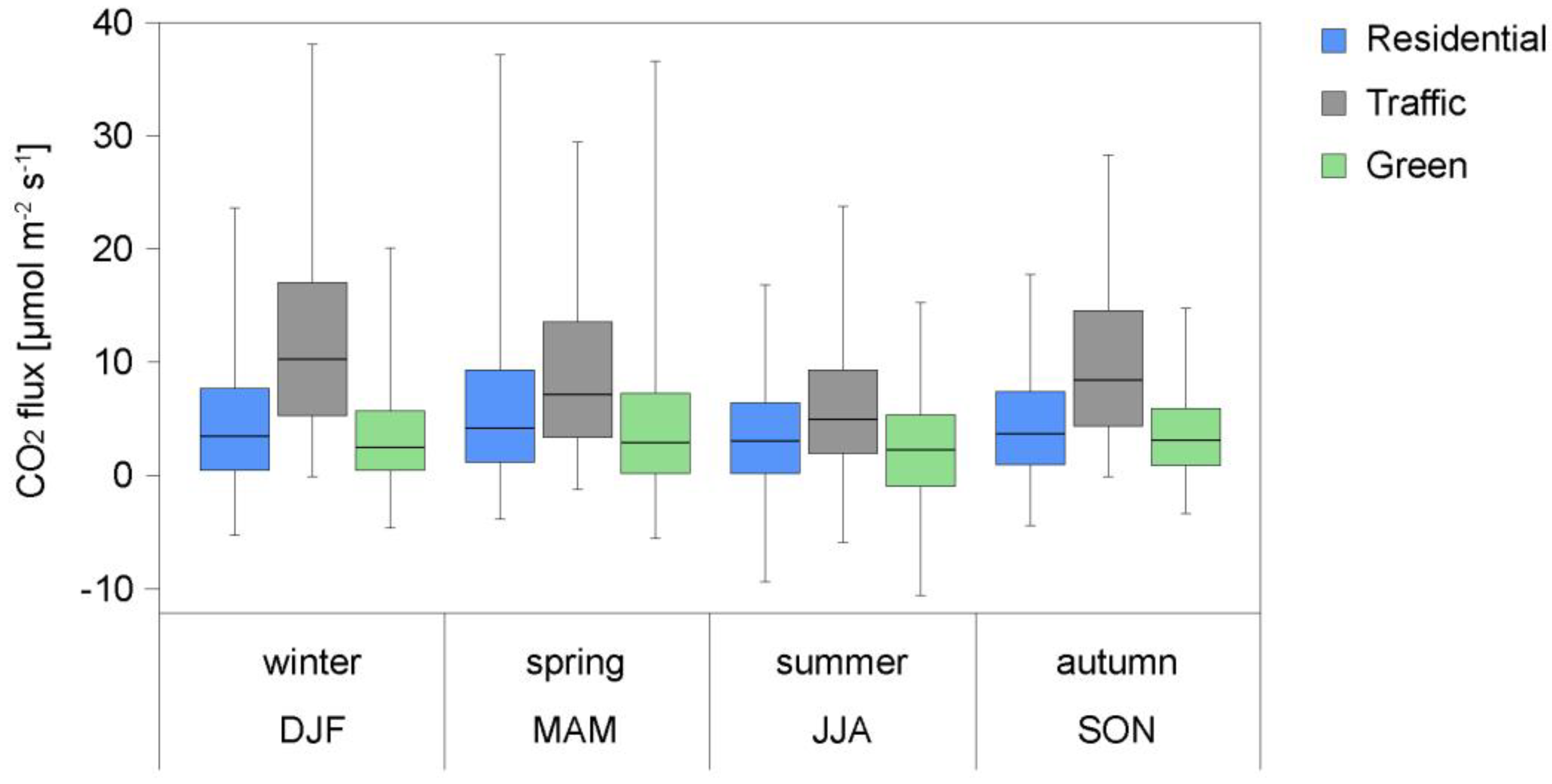
The observed flux values varied significantly with the direction. The highest observed values occurred from the traffic land-use sector, with a median of 7.68 μmol m−2 s−1. The lowest values were observed from the direction of green land-use sector, with a median of 2.65 μmol m−2 s−1 and 24% of the measured fluxes being negative. Negative values indicate net CO2 uptake. Although, under favorable conditions, i.e., in a growing season and under sufficient sunlight, urban area may become a net sink of CO2, most of the time this is not the case. Spatial inhomogeneity of the net flux was most evident in autumn and winter, when the observed CO2 influx from the traffic sector was more than twice as high as from the other directions (Figure 6).
The results obtained at the REA-AGH site are comparable with data available in the literature. In Helsinki, the seasonal average CO2 flux from various land use sectors ranged from –1.2 to 11 µmol m−2 s−1 [40]. In Łódź, one of the largest Polish cities, the most commonly occurring values were in the range of 0–15 µmol m−2 s−1, with some negative values during summer and exceeding 30 µmol m−2 s−1 during winter [41]. In London, the range of the measured net CO2 flux range was even wider: from 7 to 47 µmol m−2 s−1 [8], and in Basel from 5 to 25 µmol m−2 s−1 [42].
3.4. Urban CO2 Budget on a Local Scale
The local-scale CO2 budget (Equation (4)) was used to calculate the photosynthetic uptake from the atmosphere in a source area of the REA-AGH site (GPPU). In this equation, Fnet denotes the total net CO2 flux density measured by REA with the median of 5.71 μmol m−2 s−1. Anthropogenic emissions in Krakow as of 2010, according to the EDGAR inventory [34], are listed in Table 3. The estimated annual CO2 flux from transportation and built-up areas within the REA-AGH source area is equal to 1.37 μmol m−2 s−1 and 4.72 μmol m−2 s−1, respectively.
According to the city records [21], at the time of the study 2357 inhabitants lived within the source area of the REA-AGH site. Hence, the input to the local CO2 budget from human respiration is estimated as 1.1 μmol m−2 s−1. Two of the soil flux measurement sites were located within a short distance from the source area: S1 and S3 (Figure 2). Utilizing the data collected at those two sites, the mean soil CO2 flux density at the source area was calculated to 3.47 ± 0.28 μmol m−2 s−1. In the REA-AGH source area, the green surface fraction is 52%, so this number should be scaled-down to 1.8 μmol m−2 s−1. The GPPU calculated using Equation (4) and the estimated components is equal to 3.27 μmol m−2 s−1.
The calculation of the local photosynthetic uptake flux was performed with the assumption that local vegetation is the only source of CO2 flux recorded from the green sector of REA-AGH site source area. This assumption is not entirely met—in the green sector, greenery is dominant but not the only land-use type. There are also traffic lanes and a few institutional buildings located there (Figure 3). Therefore, a part of the recorded CO2 flux from this direction originates from sources other than vegetation. This may lead to underestimation of the calculated GPPU, as has been observed in previous studies of CO2 net flux from highly heterogeneous areas [43].
3.5. CO2 Budget for Krakow Agglomeration
According to the municipal land-use data green areas cover more than a half of the total administrative city area (Table 4; [36]). The total soil emissions of CO2 from green areas located within the city limits are equal 1.378 MtCO2 yr−1. Along with CO2 emissions from water courses in Krakow, they account for 1.389 Mt CO2 that is emitted annually to the local atmosphere (Table 4).
The above estimate was obtained based on direct measurements of surface CO2 fluxes. Therefore, it does not take into account above-ground plant emissions, as well as the CO2 photosynthetic uptake.
The assessment of local-scale CO2 budget within the REA-AGH source area resulted in photosynthetic uptake flux of 3.27 μmol m−2 s−1. Green areas occupy 53% of the surface within the administrative borders of the city, corresponding to area of 174 km2 (Table 4) therefore, in total, the city biosphere absorbs approximately 0.79 Mt CO2 annually.
As for other cities where the carbon budget was estimated, Krakow has been found to be a net source of CO2. The CO2 budget entire administrative area of the city is presented below (cf. Equation (3)):
Ftot = Ctra + Cres + Cind + Rsoil + Rriv + Rhum − GPPU
= 0.37 + 1.10 + 4.97 + 1.378 + 0.011 + 0.23 − 0.79 = 7.27 Mt CO2 yr−1.
= 0.37 + 1.10 + 4.97 + 1.378 + 0.011 + 0.23 − 0.79 = 7.27 Mt CO2 yr−1.
Several components of the net CO2 flux vary seasonally, so some variation of Ftot should be expected. Soil CO2 emissions strongly depend on the season, with temperature being the main driver: CO2 flux measured in different seasons at the same location could differ by more than one order of magnitude, with the maximum values observed in spring and summer and the minimum in winter. CO2 uptake from the local atmosphere vary seasonally as well, with the maximum occurring during spring and summer. On an annual scale, the vegetation in Krakow assimilates more than a half of biogenic CO2 (Equation (5)). In a temperate climate, the seasonal variability of energy and heat demand is pronounced as well, with both coal and natural gas consumption amplitude reaching 60% of annual average [5]. Relatively low emissions from fossil fuel burning, combined with maximum of photosynthetic uptake of CO2 in the warm season, result in a distinct minimum of the net CO2 emissions from the city. This effect has previously been shown for the CO2 concentration in the atmosphere of Krakow [3,5,44].
The Krakow municipal area produces around 7.3 Mt CO2 annually, which corresponds to a flux density of 22.3 kg CO2 m−2 yr−1, or 6.1 kg C m−2 yr−1. Similar results have been obtained for other European cities (Table 5). They are also in agreement with the prediction of a model based on satellite land cover data which estimates around 7 kg C m−2 annually for Krakow [45].
Industry is the most important source of CO2 in Krakow, accounting for 68% of the total annual emissions. Local biosphere net exchange accounts for 9% of the total emissions, with more than a half of the emitted CO2 being assimilated by the vegetation trough photosynthetic uptake. Traffic and residential sources account for 5% and 15% of the total emission, respectively. Human respiration contributes with ca. 3%, while surface waters are responsible for only a small fraction (0.1%) of the emissions.
When a fraction of green area in the city is about 80%, the urban area has the potential to become carbon-neutral, with biosphere able to assimilate all of the CO2 emitted by other local sources [45]. Out of 140 km2 of the urbanized area of the Krakow agglomeration, 89 km2 is directly built-up [36]. Assuming that all of the available roof surface is converted into green, the additional assimilation would be around 0.02 Mt CO2 annually, and the total budget would be changed only slightly. With the main source of CO2 being industry in Krakow, reducing the emissions in this part of the total carbon budget of the city seems to be the most perspective type of action towards making the city more environmentally friendly.
3.6. Uncertainty Estimation for Components of the CO2 Budget
In order to assess how uncertain the estimated GPPU and Ftot values are, the uncertainty propagation law was applied to Equations (3) and (4). For the Rsoil term, a combination of a single flux measurement uncertainty of 7.0% (with 0.05 and 0.95 percentiles equal to 0.8% and 30.4%, respectively) and the standard deviations of seasonal mean flux at sites S1 and S3 were applied to obtain the respective uncertainty value of 0.28 µmol m−2 s−1. Similarly, uncertainty of the CO2 flux from the Vistula river was calculated as 0.31 µmol m−2 s−1, with the flux results from all three measurement sites. The uncertainty of the single-point eddy covariance flux measurements have been recently assessed in Helsinki, with a recommendation for a general rule of thumb that a 12% CO2 flux bias can be applied in densely built-up areas [37]. Additional systematic errors connected with possible undetected leakages of REA system were taken into consideration as well, and, thus, the overall relative uncertainty of the Fnet in the order of 20% was assessed.
The differences between the reported emissions for the EDGAR database versions 4.2 and 5.0 were assumed as a measure of uncertainty of Ctra and Cind terms, 74% and 10% respectively. The same uncertainty was assumed for Cres term as for Cind. Human respiration term Rhum relative uncertainty was assumed to be 20%, to consider human movements and population changes in time.
Applying the above estimations and uncertainty propagation law to Equation (4), the uncertainty of photosynthetic uptake flux (GPPU) estimate was assessed as 1.62 µmol m−2 s−1 (50% relative), with the main source of uncertainty being the anthropogenic emissions inventory data. Similarly, applying the estimated uncertainty values to Equation (3), and additionally assuming that land cover data presented in Table 4 are certain, the annual CO2 emission from municipal area of Krakow was assessed as 7.27 ± 0.74 Mt CO2 yr−1.
The estimation of Rsoil term based on the chamber measurements does not take into account aboveground respiration of high-rise green. In a temperate, humid climate, deciduous forest respiration (both autotrophic and heterotrophic; both belowground and aboveground) is a source of 1048 ± 64 gC m−2 annually, and the respective value for evergreen forests is 1336 ± 57 gC m−2 yr−1 [51]. Forests cover 1731 hectares, or 5.3% of total Krakow area. According to the Regional Dictorate of the State Forests, 61.7% of that is coniferous and 38.3% is deciduous [52]. The remaining 633 ha of an area, which sums up to 23.64 km2 in Table 4, under the category forests and parks, is covered by parks and orchards, so it was assessed that a majority of tree species in this land cover is deciduous (70%) and the rest is evergreen (30%). Using the fluxes estimated by Luyssaert et al. [51] and above fractions of deciduous and evergreen species, the CO2 annual respiration of forests and parks in Krakow was assessed as 0.078 MtCO2 and 0.026 MtCO2 respectively, summing up to the total emission of 0.104 MtCO2 from tree-covered areas in the city. Since the obtained value of 0.104 Mt CO2 represents a maximum underestimation that might take place due to omitting aboveground respiration, it was assumed to be a reliable measure of this uncertainty. Hence, the total uncertainty of the CO2 flux from soils in forested areas is a combination of the uncertainty associated with the chamber flux measurements, and the uncertainty resulting from undetermined aboveground respiration, in total approximately 0.105 Mt CO2. However, due to the relatively small area covered by forests and parks, the impact of this omission on the total CO2 emission from Krakow is negligible, the difference being 0.003 Mt CO2.
The same values of forest respiration were used to assess a maximum possible photosynthetic uptake flux underestimation, due to aboveground respiration in the REA-AGH source area. Annual emissions of deciduous and evergreen forests from Luyssaert et al. [51] correspond to respective CO2 fluxes of 2.77 µmol m2 s−1 and 3.53 µmol m2 s−1. The majority of the trees are deciduous in the source area (ca. 80%), so the mean weighted flux is 2.92 µmol m2 s−1. Within 500 m radius of the measurement site, high-rise green covers 18% of the area (Figure 3), so scaling-down of this fraction was applied. The resulting respiration flux from the high-rise green in the REA source area is 0.53 µmol m2 s−1. This is a measure of potential underestimation of gross primary production. The resulting annual uptake correction due to aboveground respiration on a city scale is 0.13 Mt CO2. This is less than the assessed uncertainty of the estimated GPPU, equal to 0.40 Mt CO2 yr−1.
4. Conclusions
The CO2 flux from soils in Krakow is an important component of the city’s carbon budget. It is characterized by strong seasonal variability, with maximum values occurring in early summer and minimum during winter. The soil CO2 flux depends primarily on temperature [11] and humidity [12], but also on the soil type: at the site representing undisturbed natural soil, the highest values of soil CO2 flux were measured. Small but positive soil CO2 fluxes measured in winter confirm that soil respiration is active also during this season, despite of temperatures approaching 0 °C or being negative.
Emissions of CO2 from water courses reflect mainly the flow regime of water. Water damming has large effect on the observed emissions. The relatively small area covered by water courses within Krakow administrative borders means that the contribution of water sources to the total CO2 budget of the city is minor, accounting for only 0.1% of the total CO2 emissions annually (Table 4). However, with the flux density comparable to soil emissions, it should not be neglected in urban CO2 budgets, especially in cities with larger water bodies.
Krakow is a net source of CO2, with approximately 7.3 ± 0.8 Mt CO2 being emitted annually from the administrative area of the city. Although, under favorable conditions, the local vegetation can assimilate enough CO2 to generate negative net CO2 fluxes to the local atmosphere during summer, on the annual time-scale, it is a source of CO2, being responsible for 9% of the total emissions. Fossil fuel combustion is responsible for 88% of the total CO2 emissions in the city while the respiration of inhabitants accounts for ca. 3%. Although the CO2 budget of an urban area with a relatively high green fraction can be negative [45], for cities with strong industrial sources of CO2, achieving carbon-neutrality can be very difficult.
Author Contributions
Conceptualization, A.J.-K., M.Z., and K.R.; methodology, A.J.-K., M.Z., and P.W.; investigation, A.J.-K., M.Z., and P.W.; writing—original draft preparation, A.J.-K.; writing—review and editing, M.Z., K.R., and P.W. All authors have read and agreed to the published version of the manuscript.
Funding
This work was partially supported by the Ministry of Science and Higher Education, project No. 817/N-COST/2010/0, and project No. 16.16.220.842 B02; and European Science Foundation TTorch exchange grant No. 4705.
Acknowledgments
Authors would like to express gratitude towards Leena Järvi and Timo Vesala from Institute for Atmospheric and Earth System Research, University of Helsinki, for essential support in REA data handling, and Paweł Siedlecki from Meteorology Department, Poznań University of Life Sciences, for helping with system design and construction. We would also like to appreciate our colleagues from AGH University of Science and Technology for tremendous help with field measurement campaigns.
Conflicts of Interest
The authors declare no conflict of interest.
References
- Schneider, A.; Friedl, M.A.; Potere, D. A new map of global urban extent from MODIS satellite data. Environ. Res. Lett. 2009, 4, 44003. [Google Scholar] [CrossRef] [Green Version]
- International Energy Agency. World Energy Outlook 2008; Organisation for Economic Co-operation and Development: Paris, France, 2008; ISBN 9789264019065. [Google Scholar]
- Kuc, T.; Zimnoch, M. Changes of the CO2 sources and sinks in a polluted urban area (southern Poland) over the last decade, derived from the carbon isotope composition. Radiocarbon 1998, 40, 417–423. [Google Scholar] [CrossRef] [Green Version]
- Pataki, D.E.; Bowling, D.R.; Ehleringer, J.R. Seasonal cycle of carbon dioxide and its isotopic composition in an urban atmosphere: Anthropogenic and biogenic effects. J. Geophys. Res. 2003, 108, 4735. [Google Scholar] [CrossRef]
- Zimnoch, M.; Jeleń, D.; Gałkowski, M.; Kuc, T.; Nęcki, J.; Chmura, Ł.; Gorczyca, Z.; Jasek, A.; Różański, K. Partitioning of atmospheric carbon dioxide over Central Europe: Insights from combined measurements of CO2 mixing ratios and their carbon isotope composition. Isotopes Environ. Health Stud. 2012, 48, 421–433. [Google Scholar] [CrossRef]
- Moriwaki, R.; Kanda, M. Seasonal and diurnal fluxes of radiation, heat, water vapor and carbon dioxide over a suburban area. J. Appl. Meteorol. 2004, 43, 1700–1710. [Google Scholar] [CrossRef]
- Prairie, Y.T.; Duarte, C.M. Direct and indirect metabolic CO2 release by humanity. Biogeosciences 2007, 4, 215–217. [Google Scholar] [CrossRef] [Green Version]
- Helfter, C.; Famulari, D.; Phillips, G.J.; Barlow, J.F.; Wood, C.R.; Grimmond, C.S.B.; Nemitz, E. Controls of carbon dioxide concentrations and fluxes above central London. Atmos. Chem. Phys. 2011, 11, 1913–1928. [Google Scholar] [CrossRef] [Green Version]
- Briber, B.M.; Hutyra, L.R.; Dunn, A.L.; Raciti, S.M.; Munger, J.W. Variations in atmospheric CO2 mixing ratios across a Boston, MA urban to rural gradient. Land 2013, 2, 304–327. [Google Scholar] [CrossRef] [Green Version]
- Schüssler, W.; Neubert, R.; Levin, I.; Fischer, N.; Sonntag, C. Determination of microbial versus root-produced CO2 in an agricultural ecosystem by means of δ13CO2 measurements in soil air. Tellus B 2000, 52, 909–918. [Google Scholar] [CrossRef]
- Raich, J.W.; Schlesinger, W.H. The global carbon dioxide flux in soil respiration and its relationship to vegetation and climate. Tellus B 1992, 44, 81–89. [Google Scholar] [CrossRef] [Green Version]
- Tang, X.L.; Liu, S.G.; Zhou, G.Y.; Zhang, D.Q.; Zhou, C.Y. Soil-atmospheric exchange of CO2, CH4, and N2O in three subtropical forest ecosystems in southern China. Glob. Chang. Biol. 2006, 12, 546–560. [Google Scholar] [CrossRef]
- Zhou, W.-J.; Zhang, Y.-P.; Schaefer, D.A.; Sha, L.-Q.; Deng, Y.; Deng, X.-B.; Dai, K.-J. The role of stream water carbon dynamics and export in the carbon balance of a tropical seasonal rainforest, Southwest China. PLoS ONE 2013, 8, e56646. [Google Scholar] [CrossRef] [PubMed]
- Nimick, D.A.; Gammons, H.C.; Parker, S.R. Diel biogeochemical processes and their effect on the aqueous chemistry of streams: A review. Chem. Geol. 2011, 283, 3–17. [Google Scholar] [CrossRef]
- Raymond, P.A.; Hartmann, J.; Lauerwald, R.; Sobek, S.; McDonald, C.; Hoover, M.; Butman, D.; Striegl, R.; Mayorga, E.; Humborg, C. Global carbon dioxide emissions from inland waters. Nature 2013, 503, 355–359. [Google Scholar] [CrossRef] [PubMed] [Green Version]
- Jeleń, D. Anthropogenic Carbon Dioxide in Krakow City. PhD Thesis, University of Science and Technology, Krakow, Poland, 2012. [Google Scholar]
- Wachniew, P. Isotopic composition of dissolved inorganic carbon in a large polluted river: The Vistula, Poland. Chem. Geol. 2006, 233, 293–308. [Google Scholar] [CrossRef]
- Jasek, A.; Zimnoch, M.; Gorczyca, Z.; Smula, E.; Różański, K. Seasonal variability of soil CO2 flux and its carbon isotope composition in Krakow urban area, Southern Poland. Isotopes Environ. Health Stud. 2014, 50, 143–155. [Google Scholar] [CrossRef]
- Stewart, I.D.; Oke, T.R. Local Climate Zones for Urban Temperature Studies. Bull. Amer. Meteor. Soc. 2012, 93, 1879–1900. [Google Scholar] [CrossRef]
- IUSS Working Group WRB. World Reference Base for Soil Resources 2014, update 2015. In International Soil Classification System for Naming Soils and Creating Legends for Soil Maps; World Soil Resources Reports No. 106; FAO: Rome, Italy, 2015; ISBN 978-92-5-108369-7. [Google Scholar]
- Municipal Spatial Information System, Geodesy Department of the Municipality of Krakow. Available online: https://msip.krakow.pl/ (accessed on 20 February 2016).
- Jasek-Kamińska, A. Variability of Biogenic Carbon Dioxide Emissions and Its Stable Isotopic Composition in an Urban Area of Krakow. PhD Thesis, University of Science and Technology, Krakow, Poland, 2017. [Google Scholar]
- Kutzbach, L.; Schneider, J.; Sachs, T.; Giebels, M.; Nykänen, H.; Shurpali, N.J.; Martikainen, P.J.; Alm, J.; Wilmking, M. CO2 flux determination by closed-chamber methods can be seriously biased by inappropriate application of linear regression. Biogeosciences 2007, 4, 1005–1025. [Google Scholar] [CrossRef]
- Pihlatie, M.K.; Christiansen, J.R.; Aaltonen, H.; Korhonen, J.F.J.; Nordbo, A.; Rasilo, T.; Benanti, G.; Giebels, M.; Helmy, M.; Sheehy, J.; et al. Comparison of static chambers to measure CH4 emissions from soils. Agr. Forest Meteorol. 2013, 171–172, 124–136. [Google Scholar] [CrossRef] [Green Version]
- Hutchinson, G.L.; Livingston, G.P. Vents and seals in non-steady-state chambers for measuring gas exchange between soil and the atmosphere. Eur. J. Soil Sci. 2001, 52, 675–682. [Google Scholar] [CrossRef]
- Foken, T.; Aubinet, M.; Leuning, R. The Eddy Covariance Method. In Eddy Covariance: A Practical Guide to Measurement and Data Analysis; Aubinet, M., Vesala, T., Papale, D., Eds.; Springer: Berlin/Heidelberg, Germany, 2012; ISBN 978-94-007-2350-4. [Google Scholar]
- Grönholm, T.; Aalto, P.; Hiltunen, V.; Rannik, U.; Rinne, J.; Laakso, L.; Hyvönen, S.; Vesala, T. Measurements of aerosol particle dry deposition velocity using the relaxed eddy accumulation technique. Tellus B 2007, 59, 381–386. [Google Scholar] [CrossRef]
- Chojnicki, B.; Siedlecki, P.; Rinne, J.; Urbaniak, M.; Juszczak, R.; Olejnik, J. The methane emission measurements using relaxed eddy technique–preliminary results from Rzecin wetland. Acta Agrophysica 2010, 179, 102–112. [Google Scholar]
- Milne, R.; Mennim, A.; Hargreaves, K. The value of the β coefficient in the relaxed eddy accumulation method in terms of fourth-order moments. Bound.-Lay. Meteorol. 2001, 101, 359–373. [Google Scholar] [CrossRef]
- Amman, C.; Meixner, F.X. Stability dependence of the relaxed eddy accumulation coefficient for various scalar quantities. J. Geophys. Res. 2002, 107. [Google Scholar] [CrossRef]
- Fortuniak, K. Radiacyjne i Turbulencyjne Składniki Bilansu Cieplnego Terenów Zurbanizowanych na Przykładzie Łodzi; Wydawnictwo Uniwersytetu Łódzkiego: Łódź, Poland, 2010; ISBN 9788375253696. (In Polish) [Google Scholar]
- Mauder, M.; Foken, T. Documentation and Instruction Manual of the Eddy-Covariance Software Package TK3. Arbeitsergebnisse 2011, 46, 62. [Google Scholar]
- Kljun, N.; Calanca, P.; Rotach, M.W.; Schmid, H.P. A simple parametrisation for flux footprint predictions. Boundary-Layer Met. 2004, 112, 503–523. [Google Scholar] [CrossRef]
- Crippa, M.; Oreggioni, G.; Guizzardi, D.; Muntean, M.; Schaaf, E.; Lo Vullo, E.; Solazzo, E.; Monforti-Ferrario, F.; Olivier, J.G.J.; Vignati, E. Fossil CO2 and GHG Emissions of All World Countries–2019 Report; EUR 29849 EN; Publications Office of the European Union: Luxembourg, 2019; ISBN 978-92-76-11100-9. Available online: https://edgar.jrc.ec.europa.eu/overview.php?v=50_GHG (accessed on 21 April 2020).
- Sanchez, M.J.S.; Bhattacharya, S.; Mareckova, K. Volume 1: General Guidance and Reporting. In 2006 IPCC Guidelines for National Greenhouse Gas Inventories, Prepared by the National Greenhouse Gas Inventories Programme; Eggleston, H.S., Buendia, L., Miwa, K., Ngara, T., Tanabe, K., Eds.; IGES: Kanagawa, Japan, 2006. [Google Scholar]
- City Development Department, Municipality of Krakow, 2013. City Status Report as of 2012. Available online: https://www.bip.krakow.pl/ (accessed on 15 February 2020). (In Polish).
- Järvi, L.; Rannik, Ü.; Kokkonen, T.V.; Kurppa, M.; Karppinen, A.; Kouznetsov, R.D.; Rantala, P.; Vesala, T.; Wood, C.R. Uncertainty of eddy covariance flux measurements over an urban area based on two towers. Atmos. Meas. Tech. 2018, 11, 5421–5438. [Google Scholar] [CrossRef] [Green Version]
- Gately, C.K.; Hutyra, L.R. Large uncertainties in urban-scale carbon emissions. J. Geophys. Res.-Atmos. 2017, 122, 11242–11260. [Google Scholar] [CrossRef]
- Long, H.; Vihermaa, L.; Waldron, S.; Hoey, T.; Quemin, S.; Newton, J. Hydraulics are a first-order control on CO2 efflux from fluvial systems. J. Geophys. Res. Biogeosci. 2015, 120, 1912–1922. [Google Scholar] [CrossRef] [Green Version]
- Vesala, T.; Järvi, L.; Launiainen, S.; Sogachev, A.; Rannik, Ü.; Mammarella, I.; Siivola, E.; Keronen, P.; Rinne, J.; Riikonen, A.; et al. Surface-atmosphere interactions over complex urban terrain in Helsinki, Finland. Tellus B 2008, 60, 188–199. [Google Scholar] [CrossRef] [Green Version]
- Pawlak, W.; Fortuniak, K.; Siedlecki, M. Carbon dioxide flux in the centre of Łódź, Poland–analysis of a 2-year eddy covariance measurement data set. Int. J. Climatol. 2011, 31, 232–243. [Google Scholar] [CrossRef]
- Schmutz, M.; Vogt, R.; Feigenwinter, C.; Parlow, E. Ten years of eddy covariance measurements in Basel, Switzerland: Seasonal and interannual variabilities of urban CO2 mole fraction and flux. J. Geophys. Res.-Atmos. 2016, 121, 8649–8667. [Google Scholar] [CrossRef] [Green Version]
- Hiller, R.; McFadden, J.; Kljun, N. Interpreting CO2 fluxes over a suburban lawn: The influence of traffic emissions. Bound.-Lay. Meteorol. 2011, 138, 215–230. [Google Scholar] [CrossRef] [Green Version]
- Jasek, A.; Zimnoch, M.; Różański, K. Isotopic composition of carbon dioxide in the atmosphere of Krakow. Acta Geogr. Lodz. 2016, 104, 113–122. [Google Scholar]
- Nordbo, A.; Järvi, L.; Haapanala, S.; Wood, C.R.; Vesala, T. Fraction of natural area as main predictor of net CO2 emissions from cities. Geophys. Res. Lett. 2012, 39, 1–5. [Google Scholar] [CrossRef]
- Gioli, B.; Toscano, P.; Lugato, E.; Matese, A.; Miglietta, F.; Zaldei, A.; Vaccari, F.P. Methane and carbon dioxide fluxes and source partitioning in urban areas: The case study of Florence, Italy. Environ. Pollut. 2012, 164, 125–131. [Google Scholar] [CrossRef]
- Soegaard, H.; Møller-Jensen, L. Towards a spatial CO2 budget of a metropolitan region based on textural image classification and flux measurements. Remote Sens. Environ. 2003, 87, 283–294. [Google Scholar] [CrossRef]
- Järvi, L.; Nordbo, A.; Junninen, H.; Riikonen, A.; Moilanen, J.; Nikinmaa, E.; Vesala, T. Seasonal and annual variation of carbon dioxide surface fluxes in Helsinki, Finland, in 2006–2010. Atmos. Chem. Phys. 2012, 12, 8475–8489. [Google Scholar] [CrossRef] [Green Version]
- Kordowski, K.; Kuttler, W. Carbon dioxide fluxes over an urban park area. Atmos. Environ. 2010, 44, 2722–2730. [Google Scholar] [CrossRef]
- Magliulo, V.; Toscano, P.; Grimmond, C.S.B.; Kotthaus, S.; Järvi, L.; Setälä, H.; Lindberg, F.; Vogt, R.; Staszewski, T.; Bubak, A.; et al. Environmental measurements in BRIDGE case studies. In Understanding Urban Metabolism: A Tool for Urban Planning; Chrysoulakis, N., de Castro, E.A., Moors, E.J., Eds.; Routledge: London, UK, 2014. [Google Scholar]
- Luyssaert, S.; Inglima, I.; Jung, M.; Richardson, A.D.; Reichstein, M.; Papale, D.; Piao, S.L.; Schulze, E.-D.; Wingate, L.; Matteucci, G.; et al. CO2 balance of boreal, temperate, and tropical forests derived from a global database. Glob. Change Biol. 2007, 13, 2509–2537. [Google Scholar] [CrossRef] [Green Version]
- Forest Resources, Regional Dictorate of the State Forests. Available online: https://www.krakow.lasy.gov.pl/zasoby-lesne#.XtVa5MDgokk (accessed on 1 June 2020). (In Polish)
Figure 1.
Monthly mean air temperature and precipitation in Krakow (WMO station index: 12566) during the period of the study (2009–2014). The 30-year averages of air temperature and precipitation (1981–2010) are also shown. Horizontal axis depicts first letters of subsequent months; solid lines in the upper part of the figure depict mean monthly temperature, with an area between daily mean minimum and maximum temperatures shaded; bars and diamond markers indicate monthly precipitation. Each year of the study period is presented separately in different shades of blue, and the mean value for the study period is marked in red. Data source: Institute of Meteorology and Water Management.

Figure 2.
CO2 flux measurement locations in Krakow: soil chamber sites S1–S4 marked in green, riverine sites R1–R3 marked in blue, and relaxed eddy accumulation(REA-AGH) site marked in red. Arrow indicates river flow direction; black triangles indicate inflows of treated municipal wastewater effluents to the river (map source: Google Maps; modified).

Figure 3.
The REA-AGH site marked by black dot in the center of the map and its immediate vicinity, with established CO2 basic source types (map source: [21]).
Figure 3.
The REA-AGH site marked by black dot in the center of the map and its immediate vicinity, with established CO2 basic source types (map source: [21]).

Figure 4.
Seasonal averages of soil CO2 flux density measured at four sites (S1–S4) located in Krakow agglomeration (DJF—December, January, February; MAM—March, April, May; JJA—June, July, August; SON—September, October, December). Error bars denote standard deviation of the mean values.
Figure 4.
Seasonal averages of soil CO2 flux density measured at four sites (S1–S4) located in Krakow agglomeration (DJF—December, January, February; MAM—March, April, May; JJA—June, July, August; SON—September, October, December). Error bars denote standard deviation of the mean values.

Figure 5.
The annual mean CO2 flux density from the Vistula river measured at three sites located along the river (Figure 1). Error bars denote standard deviation of the mean values.
Figure 5.
The annual mean CO2 flux density from the Vistula river measured at three sites located along the river (Figure 1). Error bars denote standard deviation of the mean values.

Figure 6.
Box-and-whisker plot of seasonal variability of net CO2 flux density originating from different land-use sectors. Shown is median, 5–95% bars, and 25–75% boxes. Letters at the bottom of the figure denote seasons with first letters of the month (see text for details).
Figure 6.
Box-and-whisker plot of seasonal variability of net CO2 flux density originating from different land-use sectors. Shown is median, 5–95% bars, and 25–75% boxes. Letters at the bottom of the figure denote seasons with first letters of the month (see text for details).


Table 1.
Characteristics of soil CO2 flux measurement sites.
| Site | Urban Local Climate Zone 1 | Soil Type 2 | Vegetation Maintenance | pH 3 | Volumetric Porosity 4 | Carbon Content 4 [wt.%] |
|---|---|---|---|---|---|---|
| S1 | LCZ 2 | Urbisols | Regularly cut during vegetation period | 7.6 | 0.50 | 3.4 |
| S2 | LCZ D | Cambic Fluvisols | Cut upon reaching 20–30 cm in height | 7.0 | 0.51 | 3.7 |
| S3 | LCZ B | Technosols | Regularly cut during vegetation period | 7.7 | 0.50 | 2.3 |
| S4 | LCZ 6 | Hortisols | Regularly cut during vegetation period | 7.9 | 0.37 | 0.5 |
Table 2.
Characteristics of riverine CO2 flux measurement sites.
| Site | Channel Width [m] | Temperature [°C] | pH | Conductivity [mS cm−1] | Alkalinity [meq/L] | pCO2 1 [ppm] |
|---|---|---|---|---|---|---|
| R1 | 90 | 1.9–29.1 | 7.5–7.9 | 1.34–5.69 | 1.54–3.46 | 1267–5052 |
| R2 | 110 | 1.9–26.4 | 7.5–7.9 | 1.28–4.39 | 1.64–3.85 | 1132–5446 |
| R3 | 70 | 3.3–26.0 | 7.5–7.9 | 1.38–4.20 | 1.76–3.81 | 1271–5072 |
1 CO2 partial pressure in the surface layer of the water derived from alkalinity, temperature, and pH.
Table 3.
CO2 anthropogenic emissions inventory in Krakow as of 2010, according to 2019 edition of the Emission Database for Global Atmospheric Research (EDGAR) [34].
Table 3.
CO2 anthropogenic emissions inventory in Krakow as of 2010, according to 2019 edition of the Emission Database for Global Atmospheric Research (EDGAR) [34].
| Emission Category 1 | CO2 Emission [MtCO2 yr−1] |
|---|---|
| Energy and industry (1A1a, 1A2, 2A, 2B, 2C1a, 2C1c, 2C1e, 2C1f, 2C2, 2G, 3) | 4.967 |
| Transportation (1A3a, 1A3b, 1A3c, 1A3d, 1A3e) | 0.369 |
| Commercial/residential buildings and waste (1A4, 1A5, 6C) | 1.102 |
1 According to Intergovernmental Panel on Climate Change (IPCC) guidelines [35].
Table 4.
Inventory of biogenic CO2 emissions in Krakow according to land-use type.
| Land Use Category | Land Area 1 [km2] | Fraction of Total City Area 1 | Representative Site | CO2 Emission [MtCO2 yr−1] |
|---|---|---|---|---|
| Urbanized | 140.40 | 43% | - | - |
| Agricultural | 149.96 | 46% | S2 | 1.264 |
| Forests and parks | 23.64 | 7% | S1, S3 | 0.114 |
| Surface water | 5.44 | 2% | R1, R2, R3 | 0.011 |
| Other | 10.01 | 2% | - | - |
| Total | 326.85 | 100% | - | 1.389 |
1 According to municipal land-use data [36].
Table 5.
CO2 emissions from European cities reported in the literature.
| Location | CO2 Emission [kg CO2 m−2 yr−1] |
|---|---|
| London [8] | 35.5 |
| Florence [46] | 30.3 |
| Kraków (this study) | 22.3 |
| Basel [42] | 17.6–19.4 |
| Helsinki city center [45] | 17.4 |
| Copenhagen [47] | 12.8 |
| Łódź [41] | 10.8 |
| Helsinki university campus [48] | 6.5 |
| Essen [49] | 6.0 |
| Gliwice [50] | 2.8 |
© 2020 by the authors. Licensee MDPI, Basel, Switzerland. This article is an open access article distributed under the terms and conditions of the Creative Commons Attribution (CC BY) license (http://creativecommons.org/licenses/by/4.0/).
Share and Cite
MDPI and ACS Style
Jasek-Kamińska, A.; Zimnoch, M.; Wachniew, P.; Różański, K. Urban CO2 Budget: Spatial and Seasonal Variability of CO2 Emissions in Krakow, Poland. Atmosphere 2020, 11, 629. https://doi.org/10.3390/atmos11060629
AMA Style
Jasek-Kamińska A, Zimnoch M, Wachniew P, Różański K. Urban CO2 Budget: Spatial and Seasonal Variability of CO2 Emissions in Krakow, Poland. Atmosphere. 2020; 11(6):629. https://doi.org/10.3390/atmos11060629
Chicago/Turabian StyleJasek-Kamińska, Alina, Mirosław Zimnoch, Przemysław Wachniew, and Kazimierz Różański. 2020. "Urban CO2 Budget: Spatial and Seasonal Variability of CO2 Emissions in Krakow, Poland" Atmosphere 11, no. 6: 629. https://doi.org/10.3390/atmos11060629
Note that from the first issue of 2016, this journal uses article numbers instead of page numbers. See further details here.