Chemical Analysis of Surface-Level Ozone Exceedances during the 2015 Pan American Games

Abstract

Surface-level ozone (O₃) continues to be a significant health risk in the Greater Toronto Hamilton Area (GTHA) of Canada even though precursor emissions in the area have decreased significantly over the past two decades. In July 2015, Environment and Climate Change Canada (ECCC) led an intensive field study coincident with Toronto hosting the 2015 Pan American Games. During the field study, the daily 1-h maximum O₃ standard (80 ppbv) was exceeded twice at a measurement site in North Toronto, once on July 12 and again on July 28. In this study, ECCC’s 2.5-km configuration of the Global Environmental Multi-scale (GEM) meteorological model was combined with the Modelling Air-quality and CHemistry (MACH) on-line atmospheric chemistry model and the Town Energy Balance (TEB) urban surface parameterization to create a new urban air quality modelling system. In general, the model results showed that the nested 2.5-km grid-spaced urban air quality model performed better in statistical scores compared to the piloting 10-km grid-spaced GEM-MACH model without TEB. Model analyses were performed with GEM-MACH-TEB for the two exceedance periods. The local meteorology for both cases consisted of light winds with the highest O₃ predictions situated along lake-breeze fronts. For the July 28 case, O₃ production sensitivity analysis along the trajectory of the lake-breeze circulation showed that the region of most efficient O₃ production occurred in the updraft region of the lake-breeze front, as the precursors to O₃ formation underwent vertical mixing. In this updraft region, the ozone production switches from volatile organic compound (VOC)-sensitive to NOx-sensitive, and the local net O₃ production rate reaches a maximum. This transition in the chemical regime is a previously unidentified factor for why O₃ surface-level mixing ratios maximize along the lake-breeze front. For the July 12 case, differences between the model and observed Lake Ontario water temperature and the strength of lake-breeze opposing wind flow play a role in differences in the timing of the lake-breeze, which impacts the predicted location of the O₃ maximum north of Toronto.

1. Introduction

A large fraction of the world population now lives in urban areas where they are exposed to harmful air pollutants. A recent study in the U.S. showed that urban areas have up to twice the burden of asthma as compared to rural areas [1]. In addition to respiratory effects, there are cardiovascular, metabolic function, pregnancy, neurologic and psychiatric outcomes associated with human exposure to air pollution [2,3,4]. All of these effects lead to more emergency room visits, hospitalizations, absenteeism and higher health care costs. Another recent study found that paediatric asthma incidence is associated with exposure to traffic-related air pollution [5]. They estimate that 1-in-5 new cases of childhood asthma are linked to on-road mobile emissions in a large North American city. All of these recent studies highlight how urban air pollution continues to negatively impact human health.

While the mix of pollutants most responsible for health effects is still unknown, nitrogen dioxide (NO₂) has been used as a proxy for traffic-related air pollution in epidemiological studies because of the large NO_x emission (sum of oxides of nitrogen, NO+NO₂) from transportation sources and its short atmospheric lifetime [6]. The short NO_x lifetime results in large concentration gradients between urban areas and regional background conditions. Ozone (O₃) is another important component of surface-level air pollution. The Canadian Air Quality Health Index (AQHI) has two terms related to the acute human health impacts from the exposure to NO₂ and O₃ gases, as well as a term for exposure to particulate matter [7]. Odd oxygen (O_x) is defined as the sum of O₃ and NO₂. O_x has a longer lifetime in the atmosphere and can impact ecosystems on regional scales [8,9]. The spatial gradient in O_x between urban and rural areas is much weaker than NO_x because O₃ is not emitted from localized urban sources. Rather, O₃ is a secondary pollutant, which is largely dependent on chemical production and depositional loss processes. Exposure of vegetation to ground-level O₃ also leads to billions of lost revenue from lower crop yields worldwide [10].

Surface-level O₃ mixing ratios have been a challenge to control because O_x production in the lower atmosphere is a non-linear function of its precursor gases. The two classes of important precursor gases to O₃ formation are volatile organic compounds (VOCs) and oxides of nitrogen (NO_x). The precursor gases also have a wide range of emission sources, both anthropogenic and biogenic. The mixing and dilution of these precursor gases, as they transport away from their emission sources, is highly dependent on wind speed and atmospheric vertical stability. Net production of O₃ occurs in the troposphere when VOCs react with oxidants to produce peroxy radicals (RO₂), which, in turn, react with NO to form NO₂ [11]. In the presence of sunlight, the NO₂ will photolyze to form an oxygen atom that can quickly react with the abundant molecular oxygen in the troposphere to form O₃. Collectively, the availability of precursor emissions, local chemical production and dispersion (i.e., low wind speeds and vertical stability) are the key processes that impact whether O₃ mixing ratios reach unhealthy levels within and downwind of urban areas.

High concentrations of ground-level O₃ continue to be observed in the Great Lakes Region despite significant reductions in the precursor emission [12,13]. The exceedances of the national standards for O₃ in both the U.S. and Canada occur most often on hot, sunny days, downwind of the major urban areas and frequently near shorelines with well-developed lake-breeze circulations [14,15,16]. Foley et al. was one of the first comprehensive studies performed between 1994 and 2003 to measure O₃ over Lake Michigan [17]. They found that, under southwest winds, precursor emissions could be transported out over the lake where they can photochemically react to form O₃ and then can be swept on-shore in an afternoon lake-breeze. Cleary et al. measured O₃ over Southern Lake Michigan using ferry transects across and also with a shoreline-based differential optical absorption spectrometer (DOAS) instrument [18]. Ferry O₃ observations across the lake were on average 3.8 ppbv higher in O₃ than the long-path DOAS. Comparisons of the ferry measurements to community multiscale air quality (CMAQ) model predictions showed significant model over-predictions over the lake with the bias generally larger to the east side of the lake (i.e., more chemically aged air masses). More recently, McNider et al. used the WRF (weather research forecast) and the off-line CMAQ model to study the effect of mismatches between meteorological models and air-quality models using the off-line paradigm, on O₃ over-prediction over Lake Michigan. They also showed that the use of satellite-derived skin temperatures improves model predictions for temperature. Both of these factors were shown to improve their simulations of the lake-breeze circulation and atmospheric chemistry. They concluded that having a land surface scheme that can adjust moisture based on the surface energy budget is important in reducing model temperature errors [19].

Loughner et al. studied the impact of the Chesapeake Bay breeze on surface air quality in the Baltimore area [20]. On one day, they found that the convergence zone of the bay-breeze resulted in the pollution from Baltimore being transported to the upper boundary layer. Goldberg et al. found that O₃ was measured at higher concentrations over Chesapeake Bay compared to a nearby upwind site [21]. During the 10-day field study, the measured O₃ exceeded the U.S. 8-h standard on 4 different days. It was hypothesized that lower dry deposition rates, lower boundary layer heights and high photolysis rates due to clear skies over the water all contributed to the higher O₃ levels.

Southern Ontario is bounded by three of the five North American Great Lakes: Lake Huron, Lake Erie, and Lake Ontario. Sills et al. characterized lake-breeze frequency and impact on air pollution during the Border Air Quality and Meteorology (BAQS-Met) study in the Detroit/Windsor area [22]. They noted that the cool, shallow inflow to the urban boundary layer and the clear skies associated with lake-breeze days were two important factors in the concentration of precursor emissions and photochemical O₃ formation (Figure 1). Sills et al. also compared an observation-based mesoscale analyses with a high-resolution weather forecast model. The weather forecast model accurately predicted the occurrence and type of lake-breezes, but selected cases showed differences in the timing and in-land penetration of the fronts.

Brook et al. summarized air quality observations from the BAQS-Met study [23]. They concluded that the high-pressure systems associated with well-developed lake-breeze circulations could last several days, resulting in urban emissions being concentrated in the same recirculating air mass. They found that lake-driven meteorology enhances secondary pollution production and that local anthropogenic emissions have their impact closer to urban areas than would occur in the absence of the lake effects. They concluded that the presence of the large lakes causes an enhancement in the impact of local pollutant emissions on O₃.

Makar et al. showed with a chemical transport model that lake-breeze convergence zones that formed in the afternoon downwind of Detroit/Windsor confined pollutants in narrow bands horizontally (few tens of kilometers) and were locations of rapid ozone formation, though the chemistry explanation for ozone enhancement along the front was not developed in that paper [15].

Hastie et al. was one of the first studies to report the impact of a lake-breeze on the Toronto air pollution plume [24]. They observed a 30 ppbv O₃ increase in a 1-h increment at a downwind rural town associated with the passage of a lake-breeze front from Lake Ontario. Geddes et al. reported the observed trend in the daily maximum 8-h average O₃ for eight Toronto sites and showed a near zero change in this average mixing ratio between 2000 and 2007 [25]. They argued that competing effects of: (1) a small positive change in O₃ (due to NO emission deceases over the time period and a shift in O₃ photo-stationary state from NO₂ to O₃) coupled with (2) small decreases in VOC emissions (in turn decreasing the magnitude of O₃ production) resulted in near zero change in O₃ mixing ratio over the 8-year period. More recently, Pugliese et al. extended the O₃ trend for Toronto over a longer time period (2000–2012) and found a small O₃ decrease at urban and suburban sites, although decreases were not statistically significant (except for the northern suburban town of Newmarket) [26]. They also examined O₃ observations for Toronto in 2012, which was a year with a large number of O₃ exceedances. They found that year 2012 was an anomaly due to a higher-than-average number of days with light winds and winds from the west to the southeast, which cause air to be transported from other southern urban locations. There was also a higher frequency of days with stagnant wind conditions and accompanying higher-than-average frequency of clear sky days. The role of oxygenated volatile organic compounds (OVOCs) was identified as a knowledge gap due to the lack of measurements, as was the lack of data in the vertical for periods of O₃ exceedances.

Wentworth et al. assessed the impact of lake-breeze circulations on pollutants in the Greater Toronto Area using a multi-year observation data set [16]. They found that the average daily 1-h O₃ maximum was 42–49% higher on lake-breeze days. Case study analysis found that sites frequently located within the lake-breeze circulation experienced much higher O₃ than sites just outside the circulation, even though all of the sites remained within the same synoptic-scale environment that dictates long-range transport. Morning NO_x levels were greater on lake-breeze days, probably due to the stagnant, vertically stable conditions associated with lake-breeze days. They concluded that there is likely O₃-enriched air over the lake, which is transported onshore in the late morning, resulting in the high O₃ events for cities along the shoreline. Possible mechanisms were identified for high O₃ mixing ratios over the lake including: (1) reduced mixing height over the lake and near the shoreline, (2) reduced dry deposition to the lake surface, (3) a night-time land breeze that fumigates the lake surface with pollutants from the city followed by rapid O₃ production in the morning, (4) subsidence of O₃-rich air from the upper boundary layer over the lake and (5) reduced cloud cover and increased solar radiation reaching the surface over the lake. Wentworth et al. (2015) concluded that models need to represent lake-breeze circulations accurately to improve air quality predictions in the region [16].

In preparation for the July 2015 Pan American Games, held in the Greater Toronto Hamilton Area (GTHA), Environment and Climate Change Canada (ECCC) developed a suite of forecast demonstration products using the GEM (global environmental multi-scale) numerical weather prediction model as the core to the forecast systems. The demonstration forecasts included high spatial resolution forecasts for heat indices, severe weather and Lake Ontario wave heights and air quality forecasts made with the GEM-modelling air quality and chemistry (MACH) chemical transport model. The real-time, high-resolution versions of GEM showed improved forecast skill compared to the ECCC operational forecast products at the time [27].

The 2015 Pan American Games science demonstration also included an intensive meteorology and air quality field study that took place in July 2015. The summer of 2015 had two cases in the GTHA when O₃ exceeded the Ontario daily 1-h standard of 80 ppbv: 12 July and 28 July. Hence, these periods provide a valuable data set for testing meteorology and air quality model developments. The first goal of this paper is to assess the performance of the high-resolution 2.5-km GEM-MACH-town energy balance (TEB) model for predicting O₃ and NO₂ within the GTHA during the Pan American Games study. The special version of the GEM-MACH air quality model used for this study includes the town energy balance module (TEB) for urban surfaces and a high-resolution surface data assimilation scheme for updating both land and lake temperatures, as well as water vapour and surface energy fluxes at 1-h intervals. The second goal of this paper is to examine, in detail, model performance for the two O₃ exceedance periods. For the 28 July case period, a chemical coordinate analysis was performed to diagnose the chemical regime for O₃ production along the trajectory of the lake-breeze circulation. An important factor was uncovered, which contributes to the local enhancement in O₃ mixing ratio along the lake-breeze front. It was found that the vertical mixing associated with the lake-breeze front resulted in a shift in O₃ production from VOC-to-NO_x sensitive conditions. O₃ production maximizes during this chemical transition and, thus, contributes to the observed O₃ surface maximum along the lake-breeze front.

2. Experimental Methods

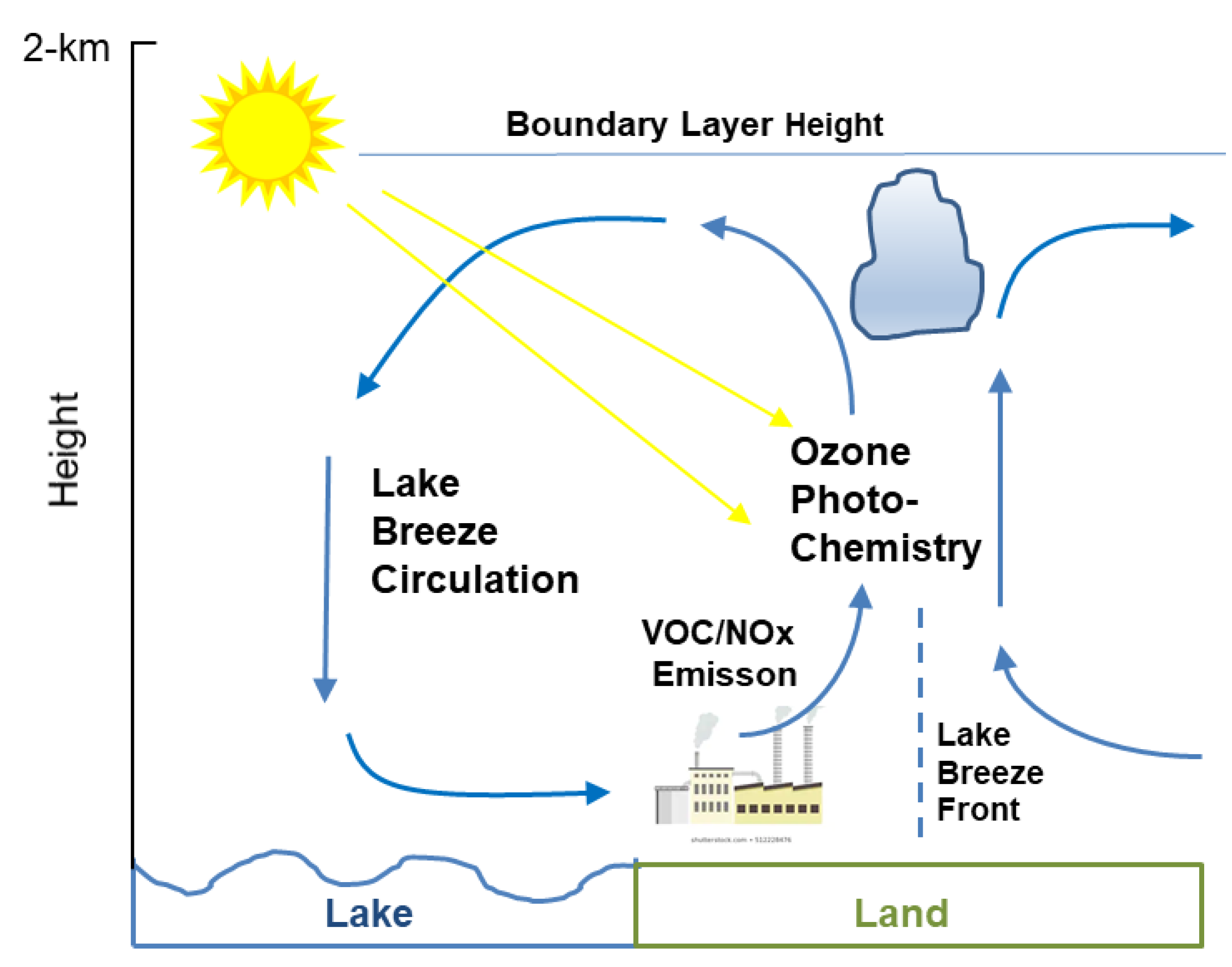
2.1. Evaluation Datasets for the 2015 Pan American Games Period

The Greater Toronto Hamilton Area (GTHA) is a region that includes both the Greater Toronto Area, located on the northwestern shore, and the city of Hamilton, located on the western shore of Lake Ontario (Figure 2). As of 2018, the population of the GTHA approached 6.8 million people and is projected to increase to 10.2 million by 2046 [28]. NO_x and VOC emissions in the GTHA are dominated by transportation, residential and commercial sources, while Hamilton also has steel production industries producing point source emissions of SO₂ and NO_x. Under prevailing summertime southwesterly winds, the GHTA is also downwind of several major U.S. cities (Chicago, Detroit and Cleveland), as well as pollution sources from the industrial Ohio Valley.

Figure 2 illustrates the 11 air quality (AQ) measurement stations active within the GTHA in 2015. These stations are part of ECCC’s National Air Pollution Surveillance (NAPS) monitoring network. One additional AQ measurement site was deployed on Toronto Island (shown on Figure 2) to support forecasting for the Pan American Games water sports. In total, there are 37 Canadian AQ stations within the 2.5-km model domain (Figure 3).

These NAPS stations continuously measure the mixing ratio of the gases O₃, NO, NO₂ and SO₂. In this study, the focus of the evaluation is on O₃, NO₂, NO_x (sum of NO + NO₂) and O_x (sum of O₃ + NO₂). In the NAPS network, O₃ is measured by UV absorption detection [29]. NO is measured by chemiluminescence detection [30]. NO₂ is measured by heated molybdenum conversion of NO₂ to NO [30,31]. An alternating inlet measures NO and then NO_x. The NO₂ is measured from the difference between NO_x and NO.

The ECCC mobile AQ laboratory (CRUISER) was deployed and made air quality measurements for several days of the Pan American Games period [27]. The CRUISER measured carbon monoxide (CO) with a UV absorption technique [32]. NO₂ and NO were measured with a selective photolytic NO₂-to-NO converter, followed by NO detection by chemiluminescence [30].

Routine surface meteorological measurements were available for sites operated permanently by the Meteorological Service of Canada (MSC). Over 40 additional compact weather stations were added in transects running north–south in Toronto [27]. The weather station data, low-level radar and GOES-13 visible satellite cloud observations were combined to form a mesoscale meteorological analysis [33]. The mesoscale analysis was used in this study to diagnose the location of lake-breeze fronts for the air quality case studies.

2.2. GEM-MACH-TEB Model Description and Setup

The GEM-MACH (global environmental multiscale–modelling air quality and chemistry) numerical model is a chemical transport model composed of dynamics, physics and atmospheric chemistry modules [34,35,36,37,38], where the chemistry modules run on-line within the GEM meteorological model [39,40]. The on-line paradigm has significant advantages over off-line models, including removal of potential interpolation errors between weather forecast and air-quality model grids, avoiding the use of conflicting boundary layer parameterizations between weather and air-quality models [19] reducing the large amount of memory space required for the storage of high resolution meteorological model output files, and reducing the overall processing time required to carry out a large domain, high resolution simulation. The on-line paradigm also enables chemistry feedbacks on weather. However, in this work, the feedback of MACH predicted aerosol on the meteorological forecast was not included. Here, we wanted to keep the MACH version similar to the ECCC GEM-MACH operational version to see the differences related to the urban canopy model and the higher spatial resolution.

Numerical modelling for the Pan American Games study was undertaken using a nested GEM-MACH domain, comprised of an outer model domain at 10-km grid spacing (750 × 620 grid cells) and an inner nested model domain at 2.5-km grid spacing (502 × 402 grid cells) centered on the GTHA. Figure 3 shows the outer GEM-MACH model domain in green and the inner 2.5-km GEM-MACH-TEB domain contoured by predicted surface O₃ mixing ratio. Both domains used the same GEM-MACH version (v2.3.1). Both GEM-MACH domains also had 80 vertical levels, up to a pressure of 0.1 hPa, and used a staggered vertical grid (based on Charney-Phillips discretization) with thermodynamic and chemical tracers on alternating levels from the dynamical tracers. In Figure 3, the 10-km GEM outer domain in blue provides the meteorological lateral boundary conditions for the 10-km GEM-MACH model (in green).

The 10-km GEM model is used to create a meteorological analysis to initialize the 10-km GEM-MACH model and 2.5-km GEM-MACH-TEB model. The surface scheme in GEM-MACH-TEB over land is based on an advanced soil moisture and land surface temperature assimilation system (termed CALDAS, Canadian Land Data Assimilation System) [41]. Hourly lake-water temperature output, for driving the GEM-MACH-TEB lake surface, comes from a 2-km coupled lake-atmosphere model system (NEMO, Nucleus for European Modelling of the Ocean). NEMO air temperature is initialized from the 10-km GEM analysis. The 10-km GEM analysis includes a surface analysis for lake temperature [42,43].

As noted above, another recent improvement to the 2.5-km GEM-MACH model was the inclusion of the town energy balance (TEB) parameterization [44,45,46]. TEB simulates the urban heat island effect more accurately by including terms in the surface heat-flux equation for building roofs, walls and road asphalt. TEB also includes the change in optical and thermal properties for urban surfaces and the change in aerodynamic roughness associated with urban buildings. Ren et al., (2020) describes the implementation of TEB into GEM-MACH [47]. A parameterization of traffic heat flux scaled from mobile pollutant emissions (as published in [48]) was used to calculate a traffic heat input into GEM-MACH using the most recent CO and NO_x mobile emission maps. For the remainder of this paper, the urbanized GEM-MACH model is referred to as GEM-MACH-TEB.

Figure 4 shows a schematic of the dynamic, physics and chemistry processes represented in GEM-MACH-TEB. GEM-MACH-TEB includes a comprehensive chemistry process package that represents gas-phase chemistry, aqueous-phase chemistry and particle microphysics (nucleation, condensation, coagulation, settling and deposition).

Table 1. High-Resolution GEM-MACH-TEB model configuration and settings used for this study.

Numerical Model Option	Option Description
Grid Spacing	2.5-km × 2.5-km
Meteorology Data Assimilation	Ensemble variational (EnVAR) method [39]
Cloud Microphysics	Milbrandt and Yau two-moment bulk [40]
Longwave Radiation	Li-Barker correlated-k distribution
Boundary Layer Scheme	TKE with statistical representation of sub-grid clouds (MoisTKE)
Cloud Convection	Kain-Fritch scheme, important for summertime convection [50]
Land Surface Scheme	ISBA and Town Energy Balance
Surface Data Assimilation	CALDAS with ensemble Kalman filtering, hourly for temperature and moisture assimilation; 2-km NEMO model for lake with 10-km analysis
Gas-Phase Chemistry	ADOM-II mechanism [51]
Gas-to-Particle Equilibrium	HETV (Heterogeneous Chemistry Vectorized)
Gaseous Deposition	Resistance model using Henry’s Law and Oxidation Potential
Photolysis Rates	Look-up table and modulation based on cloud fraction
Physics Time Step	120 s
Chemistry Time Step	240 s

lists the key model settings for chemistry and physics. The 2.5-km inner domain was initialized, based on an interpolation from the 10-km outer domain. The inner model was run in 24-h cycles with a 24-h pollutant output used to initialize the next model cycle. Biogenic emissions are calculated off-line with the BEISv3.09C (Biogenic Emission Inventory System) module [38] with updates for the biogenic emission rate for the boreal forest tree species based on a consideration of 3-year SPOT satellite-derived leaf area index (LAI) maps (see Figure A1 and

Table A1. Updates to the Biogenic Emissions Inventory System for the Canadian Boreal Forest.

	BEIS v3.09c	BEIS v3.09c	Updated	Updated	Comments
	Monoterpene µgC/m2/h	Other VOC µg/m2/h	Monoterpene µgC/m2/h	Other VOC µg/m2/h
Birch	66	408	990	140	MEGAN 2.10 [80]
Larch	33	408	1250	140	MEGAN 2.10 [80]
Pine Jack	1849	13,881	924	6941	Reduction by 2 considering satellite LAI
Populus	33	408	990	140	MEGAN 2.10 [80]
Spruce Black	3971	1620	1986	810	Reduction by 2 considering satellite LAI
Balsam Poplar/Aspen	68	408	990	140	MEGAN 2.10 [80]

). GEM-MACH v2.3.1 includes an improvement to the gas-phase dry deposition routine by assimilating LAI based on the 3-yr SPOT satellite-derived climatology. The lateral boundary conditions for the outer 10-km GEM-MACH domain were also updated by averaging the global MOZART4 model output for a summer season [49]. GEM-MACH-TEB was run on a Cray XC40 supercomputer with parallelization using a message passing interface (MPI) and OpenMP.

2.3. Pollutant Emission Inventories and Emission Processing for GEM-MACH-TEB

For the model simulations for July 2015, the 2015 Canadian National Pollutant Release Inventory (NPRI) was considered for point-source emissions, the 2015 Canadian Air Pollutant Emission Inventory (APEI) was used for area-source emissions and the 2013 APEI was considered for Canadian transportation emissions, both on-road and off-road [52,53,54]. On-road NO_x emission for Ontario’s Drive Clean Program Phase 1 area, which is approximately the area of the GTHA, from the 2013 APEI were 3869 tonnes and were created using the MOVES (mobile vehicle emission simulator) traffic emission model [55]. For the U.S., 2017 projected U.S. emissions were available, with mobile emissions also based on the MOVES traffic model. Note that total NO_x on-road emissions reported for Ohio for 2015 were 124 kt [56,57], which is comparable to our projected 2017 on-road NO_x emissions for Ohio (118 kt).

To generate 2.5-km gridded emissions for GEM-MACH-TEB, some improvements were made to the spatial surrogate fields and temporal profiles used to transform the emissions inventories into model-ready emission maps, particularly for on-road emissions. To process Canadian on-road emissions, a new set of spatial surrogates was generated using the Canadian National Road Network and population shape-files. The Canadian on-road inventory was also modified to split emissions between different road types to make better use of the new spatial surrogate fields. New diurnal profiles were used for light-duty and heavy-duty vehicles for major Canadian highways based on diesel traffic count data from a special field study [32], as described in [58]. The impact of using the new Canadian spatial surrogate fields was to redistribute the on-road mobile emissions more to the major highways and less to city streets compared to previous emissions.

In order to switch to MOVES to generate the on-road mobile emission inventories in Canada and the U.S., a new set of on-road source classification codes was introduced (2 new rural types and 2 new urban types), which required the creation of 4 new spatial surrogate fields. In addition, new off-network vehicle emission sources (from cold-starts, idling and fuel venting) were introduced with MOVES and required the creation of 11 new spatial surrogate fields (e.g., gas stations, truck stops, landfills, bus terminals and various building types). The Canadian population spatial surrogate field was also capped at 2000 people/km², based on results from [59], which show no further increase in traffic emissions with population density above this threshold. The Canadian population spatial surrogate field is used to allocate local road emissions, and having this cap reduced the on-road emissions allocated to downtown Toronto.

The new source classification codes in MOVES also enabled very detailed weekly and hourly temporal emission profiles to be created and used for the U.S. emissions (based on the U.S. Vehicle Travel Information System). A recent version of the U.S. EPA SPECIATE database (v4.5) was used for VOC and NO_x speciation profiles and applied to both the Canadian and U.S. mobile emissions [60]. The new off-network vehicle sources added with MOVES increase urban background emissions relative to previous inventories. The changes to the U.S. temporal profiles tend to increase the on-road emissions in the morning hours but reduce emissions in the afternoon rush hours and overnight [58].

The emissions of O₃ precursor species (NO_x, VOCs and CO) in Ontario and neighbouring states have decreased considerably over the past 15 years, largely due to the use of tailpipe catalytic converters on vehicles and the closure of several fossil-fuel power plants. The Supplementary includes a model emission map (Figure S1) and summaries of the emission trends over the land decade. It is interesting to look at how O₃ mixing ratios in Ontario have responded to these emission reductions [61]. Even with large emission reductions, summertime O₃ continues to exceed the 1-h 80 ppbv ambient air quality criterion, (AAQC) for O₃ (e.g., 6 times at North Toronto site in 2015). The O₃ trend in the mean concentration for the summertime months for 39 monitoring sites in Ontario increased by 3% from 2006 to 2015. The trend in the 4th highest daily maximum 8-h average O₃ mixing ratio (DM8A) from 2006 to 2015 for sites in southern Ontario decreased only 7% from 73 to 68 ppbv [62].

3. Results and Discussion

3.1. Evaluating Pollutant Emissions for a Downtown Toronto Model Grid Cell

The CRUISER mobile laboratory was deployed on 27 July 2015 with a driving route created to spatially sample throughout one 2.5-km × 2.5-km GEM-MACH-TEB grid cell (centered at 43.66° N, −79.39° W) in downtown Toronto under light southerly winds and sunny skies. The model output was extracted along the path of the CRUISER and both model and measurement time series were averaged for the time the CRUISER was within the grid cell (15:45–17:30 UTC). The median value of a running 120 s period was used to filter the CRUISER data, thus, removing points with very high concentrations that represent fresh emissions from nearby vehicles and that would not be representative of the grid-volume concentrations [63]. The time-average of the measured values for NO_x and CO was 17.6 ± 3.7 ppbv and 421 ± 12 ppbv, respectively. The modeled mixing ratios of the two species for the same period (15:45–17:30 UTC) were 19.3 ppbv and 519 ppbv, respectively, corresponding to model over-predictions of +10% and +22%. These numbers may be compared to regional AQ model evaluations in the literature [36], where North American NO₂ normalized mean biases from the GEM-MACH, WRF-CHEM and WRF-CMAQ modelling platforms ranged from 8.09% to 30.20%, NO normalized mean biases ranged from +42.15 to −61.96%, and CO normalized mean biases ranged from −7.02 to −20.09%. Urban-station-only evaluations for a European domain in the same study showed larger normalized mean biases for three different WRF-CHEM configurations (NO₂: −60.58% to −61.11%, NO: −81.46% to −86.67% and CO −34.57%). A recent global model CO intercomparison was published using satellite data, but this is not at the same scale as our study [64]. The models in this latter case had an average mean bias of −20%. The CO evaluation results shown here are considerably better than prior results with ECCC’s predecessor off-line chemical transport model (AURAMS). For a simulation of the 2007 BAQS-Met study, AURAMS CO predictions had a normalized mean bias of +134% for a measurement comparison at an urban site (Windsor) in Southern Ontario [65].

3.2. Measured O₃ Time Series in Toronto during the 2015 Pan American Games Period

Figure 5 shows the time series for modeled and measured hourly O₃ and NO₂ mixing ratio at the North Toronto measurement site for July 2015. The characteristic diurnal cycling for O₃ and NO₂ was evident. There were two periods in Figure 5a, indicated with arrows, when the observed hourly O₃ surpassed the 80 ppbv Ontario AAQC for ozone. On 28 July at 05:00 p.m. EDT, the observed O₃ reached 90 ppbv. On 12 July at 04:00 p.m. EDT (local time), O₃ reached 84 ppbv. The model under-predicted the 12 July exceedance by about 20 ppbv. It did capture the observed daytime maxima (70 ppbv) on the days before and after, and also the night-time O₃ minimum and NO₂ maximum that occurred before the exceedance. Figure 5b also includes the time series for modelled surface-level wind speed at this station. Wind speed plays a critical role in the dilution of emissions and mixing of pollutants vertically. For the two case study periods, the modelled daytime wind speeds were quite low (<4 m/s). Conversely, afternoons with modelled wind speeds >8 m/s had the lowest ozone mixing ratios. Both case study time periods will be discussed more in Section 3.4.

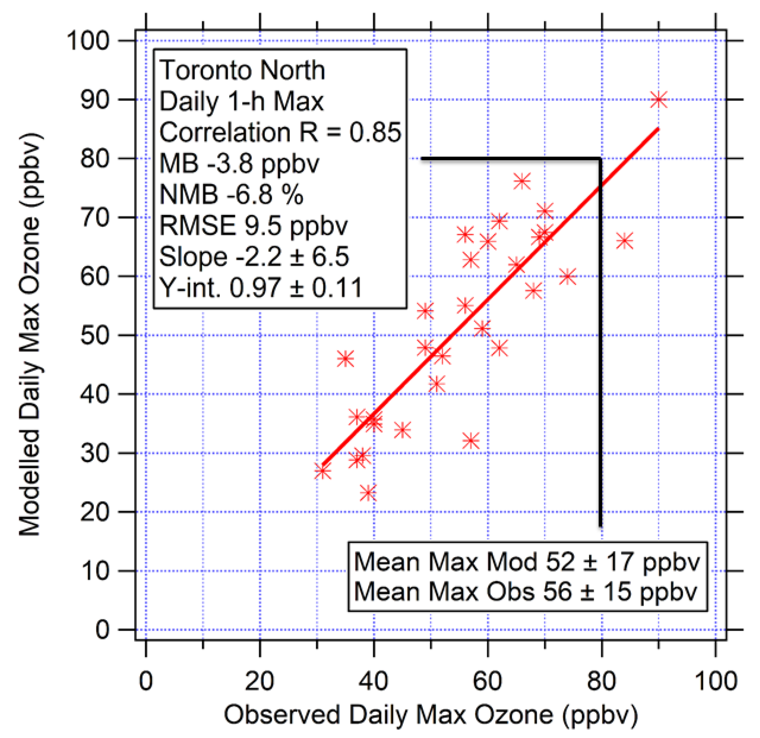
3.3. Model Evaluation

The evaluation of the 2.5-km GEM-MACH-TEB model predictions is described in detail in the Supplementary (Figures S2–S5, Tables S1–S3). Here, we briefly summarized the most important results.

Table 2. Comparison of 10-km GEM-MACH with 2.5-km GEM-MACH-TEB for 1-h data in July 2015 from all the Canadian sites in the 2.5-km domain (O₃ data is also included from U.S. AQS network). Values in red font denote better scores between the two model configurations.

Model Domain and Configuration	Metric	Observed Mean ± Standard Deviation (ppbv)	Model Mean (ppbv)	NMB (%)	Correlation Coefficient, R	RMSE (ppbv)
2.5-km GEM-MACH-TEB	O3	31.6 ± 7.5	33.3	+5.4	0.62	7.5
10-km GEM-MACH			32.6	+3.2	0.60	8.1
2.5-km GEM-MACH-TEB	NO2	6.2 ± 2.4	7.4	+18.8	0.77	3.8
10-km GEM-MACH			8.3	+34.5	0.85	4.4
2.5-km GEM-MACH-TEB	NOx	10.0 ± 4.4	10.5	+5.4	0.64	7.0
10-km GEM-MACH			11.7	+16.6	0.74	7.5
2.5-km GEM-MACH-TEB	Ox	37.7 ± 7.8	37.6	−0.34	0.80	6.8
10-km GEM-MACH			37.7	−0.18	0.81	7.3

compares the statistics for the 10-km GEM-MACH model with 2.5-km GEM-MACH-TEB for all the Canadian sites in the high-resolution 2.5-km domain (including hourly O₃ data from the U.S. Air Quality System). The 10-km model is analogous to the operational model used by the Meteorological Service of Canada for AQHI forecasting. The metrics are typical of those found in the literature to assess AQ model performance [66,67,68]; namely, normalized mean bias (NMB), root mean square error (RMSE) and the correlation coefficient (R). In looking at the NO_x statistics, the model NMB was +5.4% and correlation coefficient, R = 0.64. The O_x NMB was also very good with almost no bias, −0.3%, and a strong correlation coefficient, R = 0.80. In looking at the scores for NO₂ and O₃, there was a small O₃ over-prediction (NMB=5.4%) and a larger NO₂ over-prediction (NMB =1 9%). The RMSE for NO₂, O₃, NO_x and O_x were all lower for the high-resolution 2.5-km nested model compared to the 10-km resolution GEM-MACH piloting model. Correlation coefficient scores were slightly worse with the higher spatial resolution model for NO₂, NO_x and O_x and slightly better for O₃. Simon et al. (2012) reported RMSE values in the range, 15–20 ppbv, for hourly O₃ comparisons in other model validation studies [68], which are higher than the RMSE values here. The Supplementary section also includes a section evaluating the 2.5-km GEM-MACH-TEB model against the 10-km GEM-MACH model for all the hourly data at the 12 GTHA sites. The same conclusion was found that the higher resolution model, with the urban canopy model, outperformed the 10-km version for most statistics.

Figure 6 shows a scatterplot of the correlation between modelled and measured daily 1-h maximum O₃ at the North Toronto site for July 2015. The correlation coefficient, slope and model intercept (y-axis) were R = 0.85, 0.97 and −2.2 ppbv, respectively. The Supplementary section also included a model evaluation using the Canadian 8-h O₃ metric. Overall, results here and in the Supplementary section show that the model performance was comparable to other peer AQ models [63,66,67,68,69,70] and met the performance criteria defined in the U.S. EPA guidance documents [71,72].

The Supplementary section also included an evaluation of O_x predictions grouped according to three different wind conditions (southwesterly, northerly and light wind speeds from any direction) and two temporal periods (mid-morning and mid-afternoon). The selection of data for different wind conditions helps to separate the O_x data by source region and assess how the model performs for these different wind conditions. Figure S5 in the Supplementary section summarizes these results.

3.4. Case Study Analysis for Periods of O₃ Exceedance

In this section, the two periods with 1-h O₃ exceedances are analyzed to understand the meteorological and chemical factors that contribute to the build-up of poor air quality in Toronto. We begin in Section 3.4.1 by characterizing the synoptic-scale setup for each case by presenting U.S. NCEP (National Center for Environmental Prediction) surface reanalysis and 500-hPa height maps for North America. This is followed by plots of 48-h air mass back trajectories, derived from our 2.5-km GEM-MACH-TEB output, for the middle afternoon of each case, which allows us to characterize the origin of air masses on a regional scale. Next, Section 3.4.2 presents an analysis of pollutant time series for 4 locations, along a south-to-north transect, in the GTHA, and Section 3.4.3 presents the high-resolution pollutant surface maps, vertical cross sections, high-resolution model wind fields and the observation-derived mesoscale meteorological analysis.

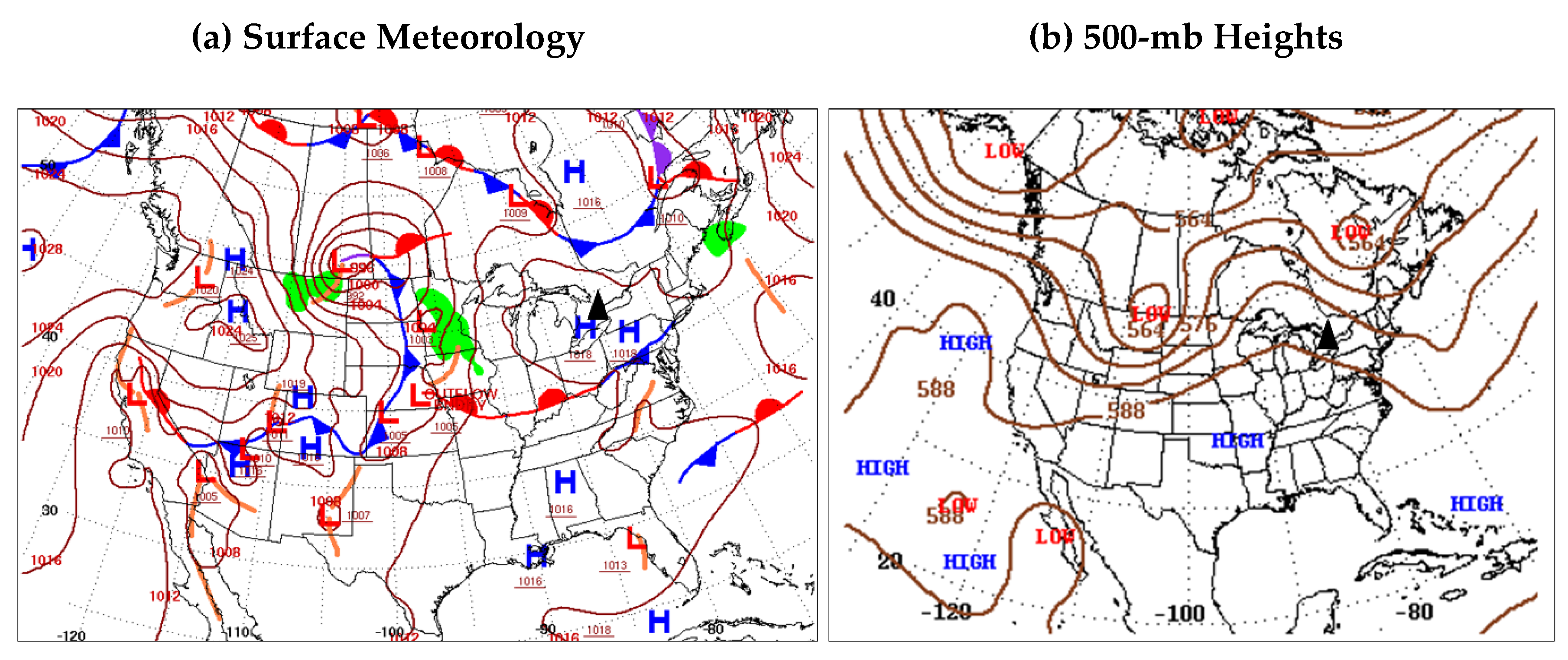
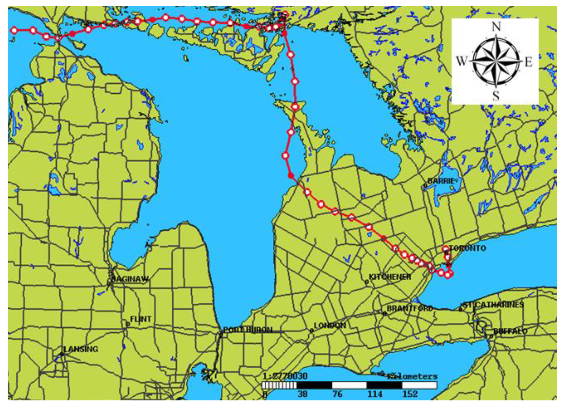
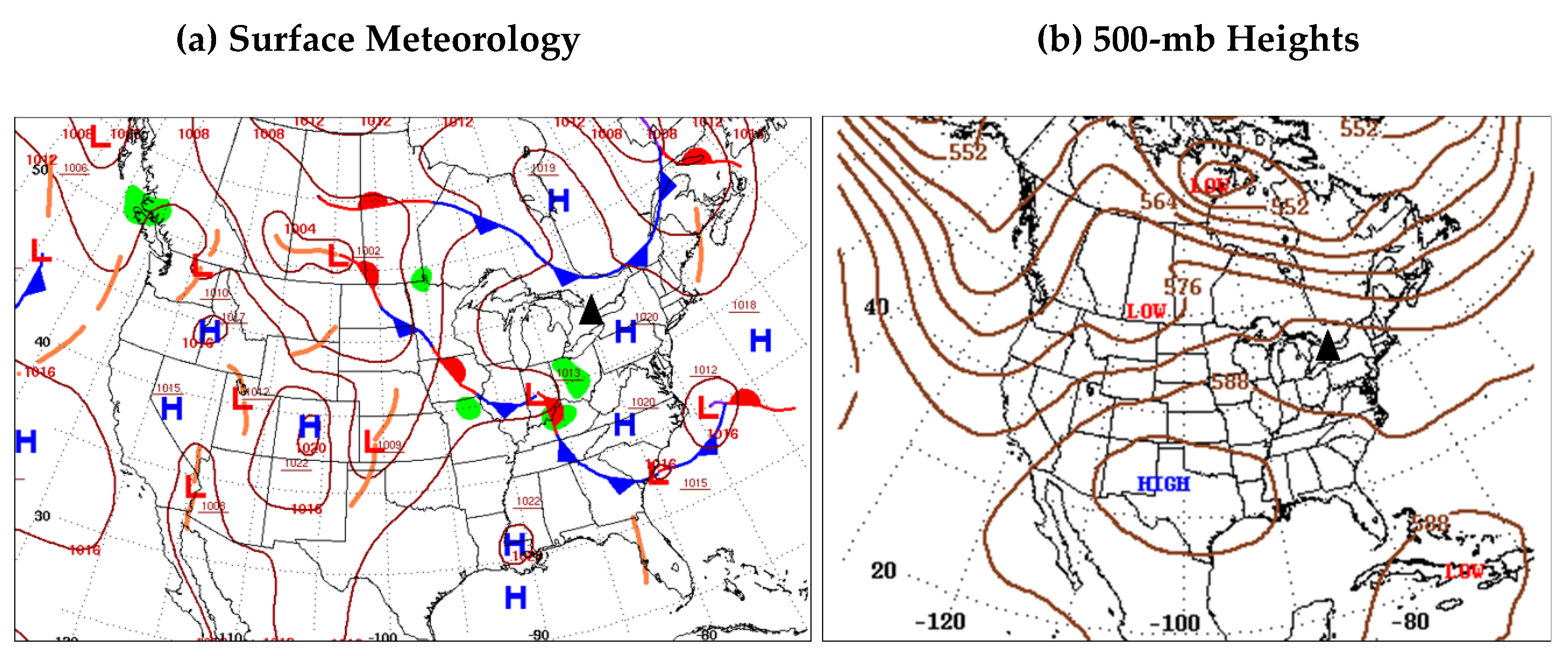
3.4.1. Synoptic-Scale Meteorology and Back Trajectories

The U.S. NCEP archives synoptic-scale reanalysis maps that show surface pressure systems and fronts each day. Geopotential heights on the 500 hPa pressure level were plotted to show the mid-troposphere jet stream. The 27 July 2015 surface map [73] has a surface high-pressure system centered over Southern Ontario. The upper-level map has a large but weak ridge building into Southern Ontario. This ridge provided for some amplification, but only small transport of surface high pressure. Figure 7 shows the surface and upper air NCEP reanalysis for 28 July 2015. A double high-pressure system has developed over Southern Ontario and Northern Pennsylvania. The upper level ridge has moved somewhat eastward into Ontario. This setup should bring air from the northern Midwest U.S. over the Great Lakes region and then SE into the GTHA. The upper-level forcing on 28 July was weak, so the surface high-pressure system did not move much throughout the daytime on 28 July.

Air mass back trajectories were calculated using the 2.5-km GEM-MACH-TEB output wind fields. Figure 8 shows the 48-h back trajectory ending in Toronto at the North Toronto station at a height of 175-m at 20:00 UTC 28 July 2015. Every point along the trajectory is a 1-h increment. For the trajectory, the time series was initialized with a height of 175-m. The trajectory starts over Northern Michigan and travels southeast over unpopulated regions of Southern Ontario before arriving over Lake Ontario. The lake breeze circulation then brings the air mass northward over downtown Toronto before arriving at North Toronto. The Supplementary section compares the 2.5-km GEM-MACH-TEB-based back trajectory with the U.S. NOAA HYSPLIT (Hybrid Single-Particle Lagrangian Integrated Trajectory) model back trajectories calculated using the 12-km NAM (North American Mesoscale) meteorological data and the 3-km HRRR (high resolution rapid refresh) meteorological data. The 2.5-km GEM-MACH-TEB back trajectory is consistent with the HYSPLIT trajectories, both of which also originate over northern Michigan.

The NCEP reanalysis map for 11 July has a surface high-pressure system over Northwestern Ohio. A weak ridge over Michigan provides for little amplification. Figure 9 shows that the surface high-pressure system has moved to Northern Pennsylvania on 12 July. The upper-level pattern on 12 July was a weak divergent zonal flow. This setup should bring air masses from the Midwest U.S. to the GTHA. The weak synoptic conditions are ideal for mesoscale features such as lake-breezes and urban heat islands to impact the local meteorology over the GTHA.

Figure 10 shows a 48-h back trajectory ending in Toronto at 20:00 UTC on 12 July 2015 based on our 2.5-km GEM-MACH-TEB wind fields. The trajectory originates over central Michigan, travels east towards Lake Ontario, passes over Lake Ontario, turns north in a lake breeze circulation, passes over downtown Toronto and finally arrives at the North Toronto station. This back trajectory is quite similar to the back trajectories calculated with the HYSPLIT model using either the 12-km NAM wind data or the 4-km HRRR data (see the Supplementary section). Note that selecting final altitudes between 50 and 300 m did not result in significant differences in the resulting back trajectories.

A 96-h HYSPLIT backward trajectory was also run for each case using the GDAS (global data assimilation system) data. Both cases were similar in that the 96-h trajectories originated from the northern Midwestern U.S. region (i.e., state of Wisconsin) and travelled over sparsely populated terrain before arriving in the GTHA. The impact from pollution sources in the Southern and Eastern U.S. are thus likely minimal. All the trajectories suggest that for both cases the enhanced pollution observed at the North Toronto site in the late afternoon is likely photochemically produced from local sources within the GTHA.

3.4.2. Case Study Time Series Analysis

Figure 11a presents the O₃ time series comparison for the 27–29 July 2015 period at the North Toronto and Newmarket measurement sites. On the afternoons of 27–28 July there was a large horizontal gradient in O₃ mixing ratio as illustrated by the 50 ppbv difference in measured O₃ between the North Toronto and Newmarket sites (a horizontal distance apart of only 30 km). This is consistent with a local influence from Toronto emissions, as also suggested by the backward trajectory for North Toronto. The model predicted the daytime O₃ maxima quite well at North Toronto on 28 July and the NO₂ maximum the night before, but under-predicted the maximum on 27 July and over-predicted the maximum on 29 July.

At the time of the 1-h O₃ exceedance in North Toronto (late afternoon on 28 July), model under-predicted at the downtown site and this under-prediction continued throughout the evening. A very stable, light-wind surface layer developed overnight and O₃ remained under-predicted throughout the night for the downtown location.

The O₃ time series between 11 and 13 July for the four sites perpendicular to the lakeshore are shown in Figure 12. The daytime O₃ maxima on July 11 were predicted well at all four sites. On 12 July, the O₃ observed at North Toronto reached over 80 ppbv in the late afternoon. At this time (20:00 UTC), the model under-predicted O₃ by 20 ppbv. The model predicted over 80 ppbv O₃ at 20:00 UTC but for the Newmarket site. The measured O₃ at Newmarket reached its maximum (73 ppbv) a couple of hours later (23:00 UTC) and the modeled O₃ at Newmarket was predicted well at 23:00 UTC. The model also under-predicted at downtown Toronto on the afternoon of 18:00 UTC 12 July. The predictions at Toronto Island did not show a strong bias in the afternoons on 11–13 July; however, the observed O₃ maxima did not exceed 65 ppbv.

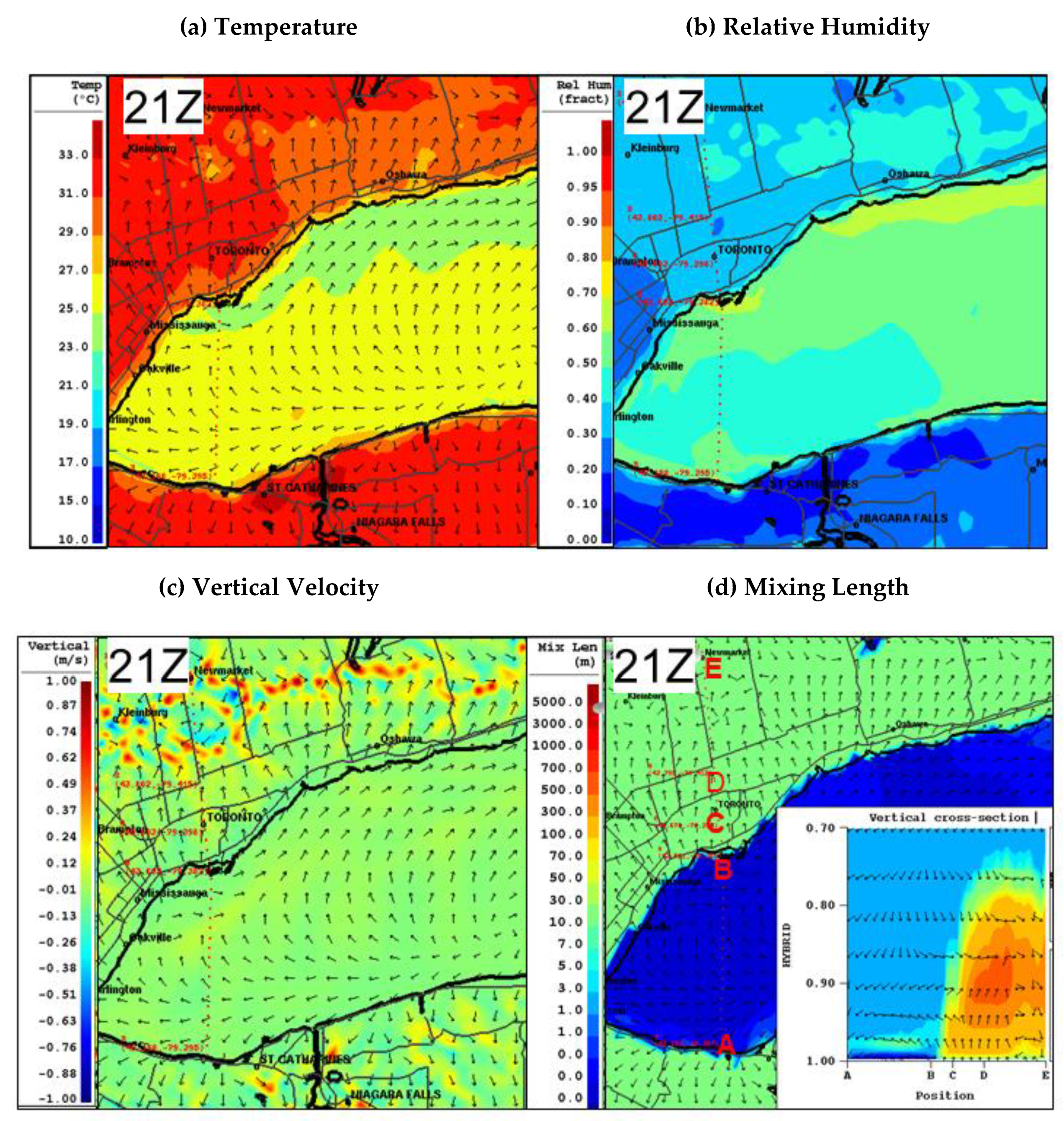
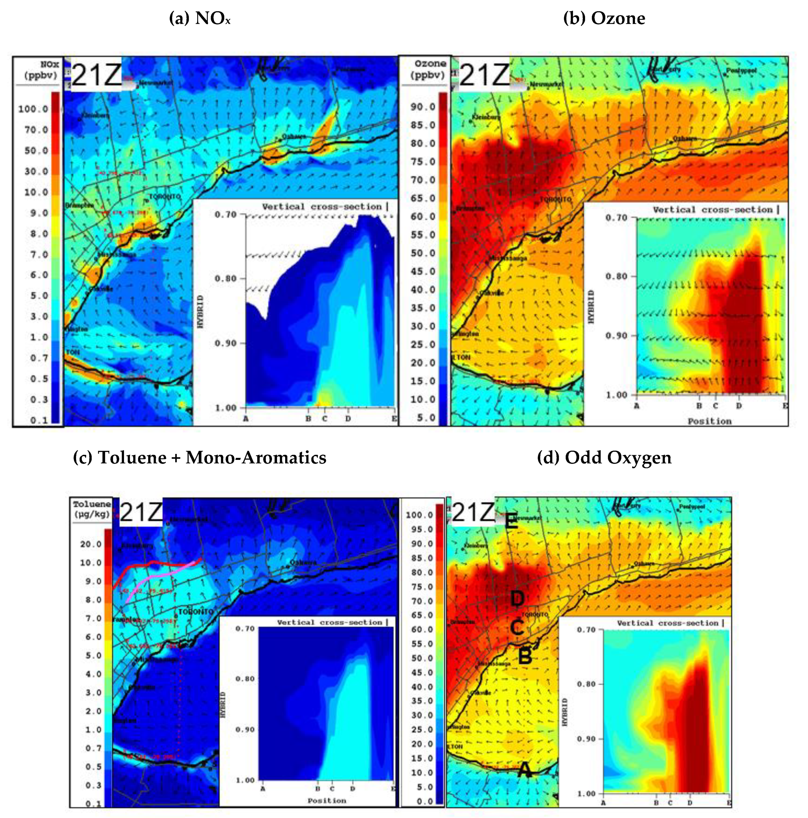
3.4.3. Modeled Pollutant Spatial Distributions, Vertical Cross Sections and Meteorological Analysis

28 July 2015 Case Study

Few observations are available in the literature on the vertical extent of lake-breeze circulations associated with O₃ exceedance periods. In this section, the modeled spatial distribution of pollutants was described for 21:00 UTC 28 July with a focus on the vertical distribution of pollutants. The Supplementary section described the meteorology and chemistry leading up to 21:00 UTC (Figures S10 and S11 at 12:00 UTC, Figures S12 and S13 at 15:00 UTC and Figures S14 and S15 at 18:00 UTC). At the end of this case study description, an O₃ sensitivity analysis was presented for 28 July at different points along the trajectory of the lake-breeze circulation. An important chemistry explanation for the O₃ maximum along a lake-breeze front would be described.

Figure 13 illustrates the temperature, relative humidity, vertical wind velocity near surface and the mixing length at 21:00 UTC (05:00 p.m. local time). The temperature over land reached a maximum up to 33 °C and the land/lake temperature difference was the maximum for the day. This temperature difference drove a strong lake-breeze front that reached as far inland as Vaughan to the north (30-km from shoreline), as illustrated by the vertical wind velocity in Figure 13c. The reader is referred to Figure 2 for the locations of cities. The vertical cross section of mixing height from Toronto Island (point A) to Newmarket (point E) shows uniformly well mixed convection all the way from point ‘C’ to point ‘E’ with mixing up to 2.3-km altitude. Horizontal winds were from the south over Toronto in the boundary layer. The lake-breeze circulation resulted in subsidence of air over Lake Ontario. A shallow layer of stable air remained over the lake surface, as shown by the dark blue color in mixing length in Figure 13d. Horizontal winds above the shallow surface layer were from the north and complete the lake breeze circulation.

A Doppler LIDAR was located at the North Toronto site on the afternoon of 28 July 2015. A description of the instrument, its deployment and the data image processing can be found in [33]. The Doppler LIDAR vertical velocity profile on 28 July at 20Z shows periods of strong up-draft followed by periods of down-draft (see Figure 6 in [27]). The up-drafts reached a maximum of 2.2-km above ground at 4 pm local time, which is the time of the lake-breeze passage. This was consistent with the height of the boundary layer predicted by GEM-MACH-TEB model and provided an independent validation of the model mixing height. The magnitude of the updrafts was similar (1 m/s) between Figure 6 in [27] and Figure 13c.

The primary emitted pollutants, NO_x and VOCs, show a uniform, well mixed region in the updraft, just south of the lake-breeze front (Figure 14). The NO_x mixing ratio is in the 3–6 ppbv range, which is optimum for efficiently producing O₃. The lumped TOLU species is in the range 1–2 ppbv throughout the updraft region. O₃ has its highest concentrations in North Toronto and Richmond Hill in the region of updraft with predicted O₃ mixing ratios of 90–95 ppbv. The region of maximum O₃ extends all the way up to 2.3-km altitude. The mixing of the O₃ with the background air was evident as the plume moves back over the lake under the northerly flow above 1-km altitude, i.e., return flow of the lake-breeze circulation. The subsidence over the lake brings cleaner air from the upper boundary layer down to the residual layer above Lake Ontario and appeared to dilute the air in the layer from 250-m to 1-km altitude above points ‘B’ to ‘C’ over Toronto Island and part of downtown Toronto (see Figure 14b). Figure 15 shows the back trajectory for 21:00 UTC 28 July 2015 for the North Toronto site. It is clear that the air traveled over the city the night before and returned over downtown Toronto in the afternoon lake-breeze circulation.

Figure 16 shows the mesoscale analysis created using data from the expanded ECCC weather station network for the study, as well as satellite and radar data. The availability of the expanded station data enables an accurate diagnosis of the location of the lake-breeze front from the observations. The observation-derived lake-breeze front at 20:00 UTC is just south of Hwy 7 and just north of the position of the CRUISER mobile vehicle location at this time. Here, the CRUISER measured up to 90 ppbv O₃, consistent with the model. The red star on Figure 16 denotes the CRUISER position at 20:00 UTC. By 21:00 UTC, the lake-breeze front is located just north of Hwy 7, passing through the city of Vaughan. Figure 14c shows the model-derived lake-breeze front on the lumped TOLU species panel (c). The gradient across the front is particularly striking for aromatic species because of their urban sources and short chemical lifetimes. The modeled lake-breeze front (red line) location is only slightly north of the observation-derived front (pink line). Both diagnosed fronts are north of the North Toronto site. The good agreement provides further validation of the modeled meteorology on 28 July 2015.

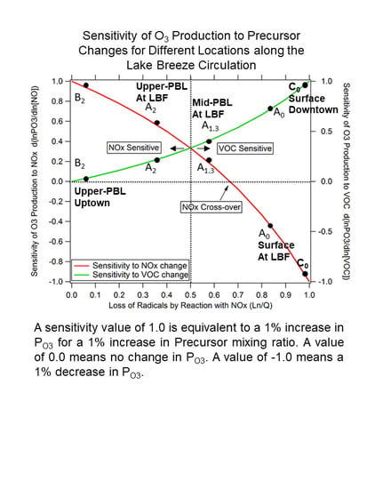
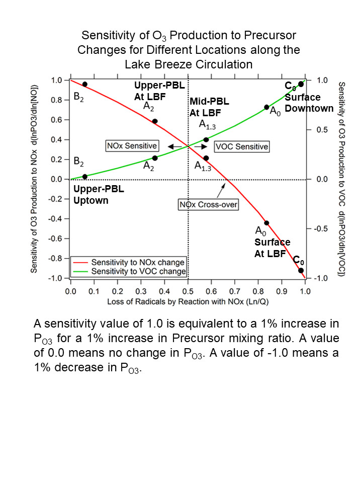
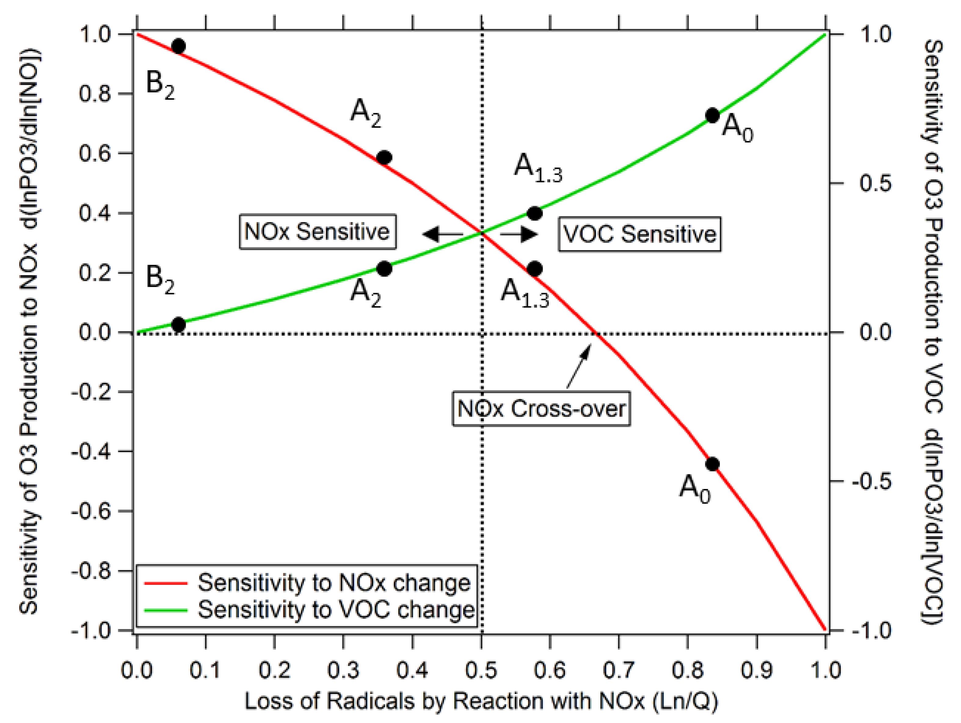
Ozone Production Sensitivity along the Lake-Breeze Air Mass Trajectory

Rapid O₃ production occurred on the afternoon of 28 July over Toronto, particularly in Uptown and North Toronto. It is informative to study the O₃ production rate sensitivity to changes in precursor concentrations, as this will shed light on the optimal emission reduction strategies to reduce O₃ mixing ratios. Kleinman et al. (2001) developed an analytical expression for the sensitivity of the O₃ production rate to changes in precursor concentrations as a function of the fraction of radicals (OH + HO₂ + RO + RO₂) that are lost by reaction with NO_x [74]. Figure 17 is a plot of the two sensitivity curves. The red curve is the O₃ production sensitivity to NO_x changes and the green curve is the sensitivity to VOC changes. The x-axis is the fraction of radicals lost by reaction with NO_x relative to the total radical loss by reactions with NO_x, HO₂ and RO₂ (termed Ln/Q). Crossing the ratio from less than 0.5 to more than 0.5 indicates a change from NOx-sensitive to VOC-sensitive O₃ production. In looking at the curve for VOC changes, the value of O₃ production sensitivity is always positive. This means that the O₃ production rate always increases with VOC increases. However, in looking at the curve for NO_x changes, the O₃ production sensitivity is positive at low Ln/Q, but turns negative at a cross-over point of Ln/Q = 0.67 and becomes increasing negative at higher Ln/Q. Figure 17 and

Table 3. Chemical coordinate analysis results for ozone production sensitivity to precursor concentration changes for different locations in lake-breeze circulation on 28 July 2015.

Chemical Sensitivity Analysis	North Toronto 20Z, Surface	North Toronto 20Z, 1.3 km	North Toronto 20Z, 2 km	Uptown Toronto 20Z, 2 km	North Toronto 18Z, Surface	Down-Town 18Z, Surface
NOx (ppbv)	5.4	3.9	2.2	0.56	12	12
Ln/Q and Sensitivity	0.84 VOC	0.59 VOC	0.36 NOx	0.059 NOx	0.88 VOC	0.96 VOC
dln(PO3)/dln(NO)	−0.45	0.16	0.56	0.94	−0.57	−0.85
dln(PO3)/dln(VOC)	0.72	0.42	0.22	0.030	0.79	0.92
OH Loss by NOx as Ratio of Total Loss	0.15	0.11	0.077	0.033	0.21	0.23
H2O2/HNO3 ratio, by mass, Sensitivity	0.253 VOC	0.246 VOC	0.301 Transition	0.702 NOx	0.348 Transition	0.356 Transition

present the results of the chemical sensitivity analysis using the model output at different locations, times and altitudes along the lake-breeze circulation.

Point A₀ on Figure 17 is the location of the CRUISER (43.80° N, 79.42° W), near the North Toronto site, when recording the 90 ppbv O₃ on at 20:00 UTC 28 July. Point A₀ refers to the ground level at point A. Point A_1.3 is at an altitude of 1.3-km above Point A. Point B is in Uptown Toronto (see Figure 2), just south of Hwy 401 (43.73° N, 79.40° W). Points A₂ and B₂ are at locations A and B, respectively, each at 2-km above ground. The analysis of the model reaction rates at point A₀ resulted in a Ln/Q value of 0.84. This corresponds to the VOC-sensitive regime with a dlnPO₃/dln(VOC) = 0.72. At this point, a 10% decrease in VOC concentration will result in a 7.2% decrease in O₃ production rate. However, in this regime, a 10% decrease in NO concentration will result in a 4.5% increase in the O₃ production rate. Above point A, at an altitude of 1.3 km, the vertical mixing is most intense resulting in a decrease in NO_x concentration because of both dilution and chemical loss. Point A_1.3 corresponds to an Ln/Q value of 0.58, just above the transition point (at 0.5) from VOC-sensitive to NO_x-sensitive conditions. This point is close to the maximum O₃ production rate for a given [VOC] reactivity (Ln/Q = 0.67 is the transition point from negative to positive value). The rapid O₃ production rate in this lake-breeze-front updraft can help to further explain why O₃ concentration maximizes along the lake-breeze convergence zone and why the high O₃ concentrations extend all the way up to 2.5-km. At point A₂, the updraft has now crossed over into the NO_x-limited regime. At this point, a 10% decrease in NO_x will result in a 6% decrease in O₃ production rate. At point B₂, there was significant dilution of plume with background air from the upper boundary layer. Point B₂ had an Ln/Q value of only 0.07. The air mass was very sensitive to NO changes and relatively insensitive to VOC changes. The modeled NO_x mixing ratios at each point in the lake-breeze circulations is also shown in Table 3. Table 3 also includes a column for downtown Toronto at surface (43.65° N, 79.38° W). The NO_x mixing ratios spanned the range from 12 ppbv downtown at surface to 0.56 ppbv uptown in the upper boundary layer.

Table 3 includes two other modeled species ratio indicators. The H₂O₂/HNO₃ ratio is a weighted measure for the O₃ production sensitivity (NO_x vs. VOC sensitive) accumulated along the history of the backward trajectory, i.e., how much of the O₃ production in an air mass has been from VOC vs. NO_x sensitive chemistry. A high H₂O₂/HNO₃ ratio (>0.6, by mass) indicates a NO_x-sensitive O₃ production regime and a low H₂O₂/HNO₃ ratio (<0.3, by mass) indicates a VOC-sensitive O₃ production regime [75,76]. In Table 3, at the surface in downtown and North Toronto, the ratio indicated a transition regime. At the North Toronto location, in the updraft, the O₃ production was VOC-sensitive and in the return flow at 2-km altitude over Uptown Toronto, the O₃ production turned to NO_x-sensitive.

There has been one recent chemical transport model study that looked at O₃ production sensitivity to precursor species. Whaley et al. (2015) used the GEOS-Chem global model to study the transport patterns for pollution events in Toronto from 2004–2007 [77]. They found that for the mid- to long-range transport cases, the O₃ maximum in Toronto was sensitive to regional-scale NO_x and isoprene emissions. For cases with stronger local O₃ production, there were high NO_x concentrations in Toronto and the local O₃ production was sensitive to anthropogenic VOC emissions in Toronto. Our high-resolution model result for light wind conditions show similar precursor sensitivity as in [77].

Finally, there are few data on OVOC contributions to total VOC reactivity for urban areas due to the challenge of measuring polar OVOCs. The OVOC/VOC ratio is the fraction of the total VOC reactivity that results from OVOC model species reacting with the OH radical. Here, we present the modeled contributions of OVOCs to the total VOC reactivity. The fraction ranged from a low of 0.28 at the downtown site to a value of 0.37 in the updraft at 2-km over North Toronto. These large fractions suggest that OVOCs are important precursors to O₃ production and the monitoring community should continue to improve network measurement methods for OVOCs.

12 July 2015 Case Study

The 2.5-km GEM-MACH-TEB model had a ‘bust’ forecast for the afternoon of 12 July 2015 when the measured O₃ exceeded 80 ppbv at the Toronto North site. In this section, we present the model-predicted spatial maps for both air quality and meteorology fields, compare them to the observation-derived mesoscale meteorological analysis, and try to answer the question as to why the model under-performed. Figure 18 presents the modeled O₃ and NO₂ surface spatial distributions at 15:00 UTC, 18:00 UTC and 21:00 UTC. The black box encompassing the downtown and North Toronto is a key region of focus. This same box is shown on the meteorological mesoscale analysis (Figure 19), and the model 10-m wind field panels (Figure S16). At 15:00 UTC, the model predicted a moderate southwesterly wind over Lake Ontario. Southwesterly winds also characterized most of the key region (black box) with the exception of the northwest corner of the box, where the model winds were more southerly, and the most southern part of the box, where a lake breeze front was just pushing on-shore. NO₂ predictions were highest over the southern portion of the box due to the urban emissions. By 18:00 UTC, the model predicted the southwesterly flow for the left half of the box and moderate southerly lake breeze flow on the right half of box. The modeled lake-breeze front arrived at Newmarket, as shown by the jump in O₃ mixing ratio in the time series (Figure 12), just after 18:00 UTC. The region of maximum ozone production was already north of Toronto. By 21:00 UTC, the model predicted over 90 ppbv O₃ north of Newmarket as the modeled lake-breeze front reached all the way to Lake Simcoe.

We next compared the model meteorology with observations to understand what caused the ‘bust’ O₃ forecast. Figure 19 shows the observation-derived mesoscale meteorological analysis from the over 40 meteorological stations. Key stations within the box were A4T (Brampton) in the west of the box, YYZ (Pearson International Airport) in the southwest of the box, King City (L2D) and Vaughan (A2T) in the north of the box and Concord (L1F) and Downsview Park (L1E) in the center of the box. At 15:00 UTC, Brampton measured the southwesterly flow, King City measured the westerly flow and the stations in the center of the box measured the light northerly flows. Pearson International Airport also measured the light northerly flow. By 17:00 UTC, the observed lake-breeze front had moved past Downsview Park and was south of Concord station. The lake-breeze front had also passed Pearson International Airport, while Brampton and King City were still reporting a southwesterly flow. By 18:00 UTC, the observed lake-breeze front had slowed its progression and was still located south of Concord. By 19:00 UTC, the front had stalled. However, by 21:00 UTC, the front had continued its progression and was now located just south of King City. By 22:00 UTC, the front had passed King City and was over Newmarket. The passage of the front at Newmarket on the mesoscale meteorological analysis was coincident with the measured O₃ maximum at Newmarket on Figure 12.

Figure S16 shows the detailed predicted surface wind fields at different times. These panels were used with the mesoscale meteorological analysis to create

Table 4. Modelled and measured time of lake-breeze passage for locations north of Toronto on 12 July 2015.

Location	Latitude, Longitude	Distance from Lake Ontario AXYZ Buoy (km)	Observed Time of Lake Breeze Passage (UTC)	Modelled Time of Lake Breeze Passage (UTC)
Downsview Park, L1E	43.75, 79.48	18	17	17
York University	43.78, 79.49	23	18	17
Concord Station L1F	43.82, 79.52	28	20	18
Vaughan Station A2T	43.86, 79.54	33	21	18
Newmarket	44.04, 79.48	51	22	19

, which compares the times of lake-breeze passage from the model and from observations along the south–north line from the lakeshore. There was a 2-h difference in the timing of the lake-breeze front passing Concord (center of box on plots). By the time the front reached Newmarket, there was a 3-h difference. The consequence of this difference in timing is that the model predicted its daytime O₃ maximum too far north (Newmarket) compared to the observed location of the O₃ maximum (North Toronto). Figure 20 shows a 24-h air-mass back trajectory arriving at Newmarket at 21:00 UTC. It is clear that the origin of the air mass earlier in the day was over Lake Ontario.

A key question to answer is why does the model predict a stronger lake-breeze flow on this afternoon? The model could differ in two potential ways. The modeled regional scale wind pattern opposing the lake-breeze front could differ from observations and/or the modeled lake/land temperature contrast could differ from observations. Figure S16 shows the predicted wind fields at 16:00–17:00 UTC. The model predicted a southwesterly flow coming into the box and southwesterly flow north of Toronto, whereas the mesoscale meteorological analysis had a weak northerly flow north of Toronto at Concord (L1F) and Vaughan (A2T) at these times. Thus, in reality on the regional scale, there was a more opposing flow to the passage of lake-breeze front.

Table 5. Modelled and measured temperatures over Lake Ontario on 12 July 2015.

Location	Time (UTC)	Model State (°C)	Observed State (°C)
Watchkeeper Buoy Station AXYZ	15:00 17:00	T water 18.1 T water 18.1	T water 19.9 T water 19.7
West Lake Buoy	15:00 17:00 19:00	T air 20.1 T air 20.0 T air 21.0	T air 22.8 T air 22.7 T air 23.1
West Lake Boat	13:00	T air 19.5	T air 21.0
Toronto Island Station YTZ	15:00 17:00	T air 20.6 T air 21.7	T air 20.9 T air 22.7

presents the modelled values for lake water (T_w) and lake air (T_air) temperatures compared to observations. There was a Watch Keeper buoy just south of Toronto Island, which measured T_w. The modeled T_w was almost 2 °C colder than that measured on the afternoon of 12 July. There was also a buoy in Southwestern Lake Ontario that recorded T_air over 2 °C warmer than the model predictions, and there was a boat deployed at a location in Western Lake Ontario that measured T_air 1.5 °C warmer than the model at its location. Finally, Toronto Island airport measured T_air slightly higher (0.3–1.0 °C) than model values on this afternoon. The wind speeds modeled at Toronto Island Airport (YTZ) were 7–9 knots (3.6–4.6 m/s) between 15:00 and 17:00 UTC. The wind speed observations at YTZ were 4–6 knots (2.0–3.1 m/s) between 15:00 and 17:00 UTC. Collectively, these results suggest the modeled T_w and T_air were cooler than the measurements in the western part of Lake Ontario. The surface scheme in 2.5-km GEM-MACH-TEB used the 2-km coupled NEMO atmosphere-lake model output over the Great Lakes. NEMO T_air was initialized from the 10-km GEM regional model meteorology [42,43]. The 10-km regional GEM model was initiated each cycle with a 10-km surface analysis, including lake T_w. A 6-h spin-up of the 2-km NEMO was used before extracting the lake T_w field for the driving 2.5-km GEM-MACH-TEB surface.

The satellite imagery on the mesoscale meteorological analysis maps suggests 12 July was a partly cloudy day over Lake Ontario. The heterogeneity in surface solar heating from broken cloud cover may have been a challenge for the NEMO model to represent on this afternoon. On 28 July, there were clear skies all morning and afternoon over Lake Ontario. In conclusion, model comparison with observations suggest the stronger modeled lake breeze on 12 July and the different timing of the front passage is due to a weak but opposing wind flow north of Toronto and a larger modeled difference in the land-lake temperature. Further improvements to the model system should consider a high-resolution, more frequent lake-water-temperature-analysis based on satellite observations. The recent McNider et al. study showed a strong sensitivity of air quality predictions on their satellite data-assimilated lake water temperatures [19].

3.5. Recommendations for Emission Reduction Strategies

Geddes et al. (2009) found that simultaneous reductions in observed mixing ratios of both VOCs and NO_x in Toronto from 2000 to 2007 did not result in a significant change in observed O₃ mixing ratios [25]. They showed using a chemical box model that this weak response was not unexpected, due to the non-linear nature of O₃ production. They also showed that, for average conditions in downtown Toronto, the O₃ production is VOC-limited. They recommended that VOC emission reductions would be most effective at decreasing local O₃ production rates. One caveat, in this prior study, was the use of 24-h VOC canister data as no high-temporal-resolution VOC data sets were available for the photochemically active times of the day. The OVOC data were also limited. They also noted the challenge in the future in reducing VOC levels as a significant fraction are biogenic in nature and biogenic emissions will likely increase in a warming climate. Makar et al. (2010) examined the sensitivities of different VOCs towards ozone formation, noting that the products of aromatic oxidation had the largest impact on urban ozone concentrations in the Great Lakes region and suggested that a reduction in on-road and shipping VOC emissions (the largest local sources of aromatics) could be one route for reducing ozone concentrations [15].

The two 1-h exceedance periods presented here are remarkably similar in terms of the meteorological setup on the synoptic scale. Based on the back trajectories, the model suggests the production of O₃ in North Toronto on these days is largely from local production. Differences in the extent of northern encroachment of the modelled lake-breeze front on each day determines which northern suburbs are affected by the maximum O₃, but both cases predict rapid production of O_x up to 90 ppbv at the front. The chemical sensitivity analysis suggests that the O₃ production is VOC-sensitive. Thus, reductions in VOC emissions over Toronto along the path from downtown to North Toronto will be most effective in reducing the rapid O₃ production rates. Indeed, conditions are NO_x saturated, in that reductions in NO_x emissions will likely increase O₃ production rates along the case study trajectories over Toronto. However, as the Toronto air mass mixes with background air from aloft, the plume will turn from VOC-sensitive to NO_x-sensitive. It seems the most prudent strategy is to reduce both urban VOC and NO_x emissions, but to reduce the urban VOC emissions more aggressively so that urban O₃ production is not enhanced further.

4. Conclusions

The first goal of this work was to evaluate 2.5-km GEM-MACH-TEB model predictions against observations for the daily maximum O₃ metric in the GTHA. The 2015 Pan American Games had 4 days in the month of July with a daily maximum 8-h average (DM8A) O₃ mixing ratio above the Canadian standard of 63 ppbv and 2 days with O₃ above the Ontario daily 1-h standard of 80 ppbv. Overall, the model performed well, with its O₃ predictions meeting the performance criteria set by the U.S. EPA. During the study, an additional measurement site was located on Toronto Island about 2-km off-shore from downtown Toronto. The model did not over-predict O₃ at this location, unlike previous model studies, including previous versions of GEM-MACH. During the study, the two highest 1-h O₃ measurements were observed farther inland along the lake-breeze front in the late afternoon. The two periods when O₃ levels were above the 1-h standard were analyzed in detail.

For 12 July, at midday, GEM-MACH-TEB predicted a strong lake-breeze front that pushed northward and that by 18:00 UTC was located north of Newmarket. However, the observation-derived mesoscale analysis diagnosed the lake-breeze front location at 18:00 UTC to be about 30 km south of Newmarket, near the town of Vaughan. The northwesterly flow, observed at the A2T station in Vaughan, also disagrees with the strong modeled southerly flow at this location. By 21:00 UTC, the modelled lake-breeze front was predicted to have reached Lake Simcoe, whereas the mesoscale analysis diagnosed the lake-breeze-front location as still south of Newmarket. This case illustrates the challenge in predicting the in-land penetration of a lake-breeze front when the synoptic forcing is weak and there is a tenuous balance of mesoscale forces resulting from land/lake temperature differences, the urban heat island, and topography changes. The model did predict the fine-scale structure and resulting O₃ maximum, but the structure was displaced northward. We identified modelled lake air and water temperatures that were too cool as a factor contributing to the difference in strength and timing of the lake-breeze front.

For 28 July, the coupled high-resolution meteorology/chemistry/urban canopy model was successful at predicting the location of the daytime O₃ maximum because the model was able to predict the location of the lake-breeze front in the afternoon. An important factor for the O₃ maximum along lake-breeze fronts was discovered when performing the O₃ production sensitivity analysis at different points along the trajectory of the lake-breeze circulation. In the shallow inflow region of the lake-breeze circulation over downtown Toronto, O₃ production is VOC-limited and suppressed by the high NO_x conditions. However, in the updraft region of the lake-breeze frontal zone, the primary pollutant concentrations begin to dilute and the O₃ production begins to transition from VOC-sensitive to NO_x-sensitive. In this transition zone, O₃ production efficiency is a maximum and the still relatively high urban VOC and NO_x absolute concentrations result in large O₃ production rates and the maximum in O₃ mixing ratios.

In general, the model results from the Pan American Games period showed that the high-resolution urbanized GEM-MACH-TEB model performed better in statistical scores (RMSE, MB) compared to the 10-km GEM-MACH model for O₃ and NO₂. The 10-km model performed slightly better for the correlation coefficient (R), likely due to the challenge in modelling the correct location of more spatially resolved pollution plumes. Future work will evaluate the high-resolution urbanized model, run in near-real time, for an entire year period against ECCC’s operational air quality model.

References

1. Alotaibi, R.; Bechle, M.; Marshall, J.D.; Ramani, T.; Zietsman, J.; Nieuwenhuijsen, M.J.; Khreis, H. Traffic related air pollution and the burden of childhood asthma in the contiguous United States in 2000 and 2010. Environ. Int. 2019, 127, 858–867. [Google Scholar] [CrossRef] [PubMed]
2. Thurston, G.D.; Kipen, H.; Annesi-Maesano, I.; Balmes, J.; Brook, R.D.; Cromar, K.; De Matteis, S.; Forastiere, F.; Forsberg, B.; Frampton, M.W.; et al. A joint ERS/ATS policy statement: What constitutes an adverse health effect of air pollution? An analytical framework. Eur. Respir. J. 2017, 49, 1600419. [Google Scholar] [CrossRef] [PubMed] [Green Version]
3. Moulton, P.V.; Yang, W. Air pollution, oxidative stress, and Alzheimer’s disease. J. Environ. Public Health 2012, 2012, 472751. [Google Scholar] [CrossRef] [PubMed]
4. Kilian, J.; Kitazawa, M. The emerging risk of exposure to air pollution on cognitive decline and Alzheimer’s disease—Evidence from epidemiological and animal studies. Biomed. J. 2018, 41, 141–162. [Google Scholar] [CrossRef]
5. Achakulwisut, P.; Brauer, M.; Hystad, P.; Anenberg, S.C. Global, national, and urban burdens of paediatric asthma incidence attributable to ambient NO2 pollution: Estimates from global datasets. Lancet Planet. Health 2019, 3, e166–e178. [Google Scholar] [CrossRef] [Green Version]
6. Levy, I.; Mihele, C.; Lu, G.; Narayan, J.; Brook, J.R. Evaluating multipollutant exposure and urban air quality: Pollutant interrelationships, neighborhood variability, and nitrogen dioxide as a proxy pollutant. Environ. Health Perspect. 2014, 122, 65–72. [Google Scholar] [CrossRef] [Green Version]
7. Stieb, D.M.; Burnett, R.T.; Smith-Doiron, M.; Brion, O.; Hwashin, H.S.; Economou, V. A new multipollutant no-threshold air quality health index based on short-term associations observed in daily time-series analyses. J. Air Waste Manag. Assoc. 2008, 58, 435–450. [Google Scholar] [CrossRef] [Green Version]
8. Clapp, L.J.; Jenkin, M.E. Analysis of the relationship between ambient levels of O3, NO2 and NO as a function of NOx in the UK. Atmos. Environ. 2001, 35, 6391–6405. [Google Scholar] [CrossRef]
9. Brown, S.S.; Ryerson, T.B.; Wollny, A.G.; Brock, C.A.; Peltier, R.; Sullivan, A.P.; Weber, R.J.; Dubé, W.P.; Trainer, M.; Meagher, J.F.; et al. Variability in nocturnal nitrogen oxide processing and its role in regional air quality. Science 2006, 311, 67–70. [Google Scholar] [CrossRef]
10. Avnery, S.; Mauzerall, D.L.; Liu, J.; Horowitz, L.W. Global crop yield reductions due to surface ozone exposure: 1. Year 2000 crop production losses and economic damage. Atmos. Environ. 2011, 45, 2284–2296. [Google Scholar] [CrossRef]
11. Jacobson, M. Fundamentals of Atmospheric Modeling, 1st ed.; Cambridge Press: Cambridge, UK, 1999; pp. 318–351. [Google Scholar]
12. MOECC. Air Quality in Ontario Report. Ontario Ministry of the Environment and Climate Change. 2016. Available online: http://www.airqualityontario.com/press/publications.php (accessed on 26 August 2019).
13. U.S. EPA. Our Nation’s Air, United States Environmental Protection Agency. 2018. Available online: https://gispub.epa.gov/air/trendsreport/2018/#home (accessed on 10 September 2019).
14. Lennartson, G.J.; Schwartz, M.D. The lake breeze-ground-level O3 connection in eastern Wisconsin: A climatological perspective. Int. J. Climatol. 2002, 22, 1347–1364. [Google Scholar] [CrossRef] [Green Version]
15. Makar, P.A.; Zhang, J.; Gong, W.; Stroud, C.; Sills, D.; Hayden, K.L.; Brook, J.; Levy, I.; Mihele, C.; Moran, M.D.; et al. Mass tracking for chemical analysis: The causes of ozone formation in southern Ontario during BAQS-Met 2007. Atmos. Chem. Phys. 2010, 10, 11151–11173. [Google Scholar] [CrossRef] [Green Version]
16. Wentworth, G.R.; Murphy, J.G.; Sills, D.M.L. Impact of lake breezes on ozone and nitrogen oxides in the Greater Toronto Area. Atmos. Environ. 2015, 109, 52–60. [Google Scholar] [CrossRef]
17. Foley, T.; Betterton, E.A.; Robert Jacko, P.E.; Hillery, J. Lake Michigan air quality: The 1994–2003 LADCO Aircraft Project (LAP). Atmos. Environ. 2011, 45, 3192–3202. [Google Scholar] [CrossRef]
18. Cleary, P.A.; Fuhrman, N.; Schulz, L.; Schafer, J.; Fillingham, J.; Bootsma, H.; McQueen, J.; Tang, Y.; Langel, T.; McKeen, S.; et al. Ozone distributions over southern Lake Michigan: Comparisons between ferry-based observations, shoreline-based DOAS observations and model forecasts. Atmos. Chem. Phys. 2015, 15, 5109–5122. [Google Scholar] [CrossRef] [Green Version]
19. McNider, R.T.; Pour-Biazar, A.; Doty, K.; White, A.; Wu, Y.; Qin, M.; Hu, Y.; Odman, T.; Cleary, P.; Kniing, E.; et al. Examination of the physical atmosphere in the Great Lakes region and its potential impact on air quality-Overwater stability and satellite assimilation. J. Alied Meteorol. Climatol. 2018, 57, 2789–2816. [Google Scholar] [CrossRef]
20. Loughner, C.P.; Tzortziou, M.; Follette-Cook, M.; Pickering, K.E.; Goldberg, D.; Satam, C.; Weinheimer, A.; Crawford, J.H.; Kna, D.J.; Montzka, D.D.; et al. Impact of bay-breeze circulations on surface air quality and boundary layer export. J. Alied Meteorol. Climatol. 2014, 53, 1697–1713. [Google Scholar] [CrossRef] [Green Version]
21. Goldberg, D.L.; Loughner, C.P.; Tzortziou, M.; Stehr, J.W.; Pickering, K.E.; Marufu, L.T.; Dickerson, R.R. Higher surface ozone concentrations over the Chesapeake Bay than over the adjacent land: Observations and models from the DISCOVER-AQ and CBODAQ campaigns. Atmos. Environ. 2014, 84, 9–19. [Google Scholar] [CrossRef] [Green Version]
22. Sills, D.M.L.; Brook, J.R.; Levy, I.; Makar, P.A.; Zhang, J.; Taylor, P.A. Lake breezes in the southern Great Lakes region and their influence during BAQS-Met 2007. Atmos. Chem. Phys. 2011, 11, 7955–7973. [Google Scholar] [CrossRef] [Green Version]
23. Brook, J.R.; Makar, P.A.; Sills, D.M.L.; Hayden, K.L.; McLaren, R. Exploring the nature of air quality over southwestern Ontario: Main findings from the Border Air Quality and Meteorology Study. Atmos. Chem. Phys. 2013, 13, 10461–10482. [Google Scholar] [CrossRef] [Green Version]
24. Hastie, D.R.; Narayan, J.; Schiller, C.; Niki, H.; Shepson, P.B.; Sills, D.M.L.; Taylor, P.A.; Moroz, W.M.J.; Drummond, J.W.; Reid, N.; et al. Observational evidence for the impact of the lake breeze circulation on ozone concentrations in Southern Ontario. Atmos. Environ. 1999, 33, 323–335. [Google Scholar] [CrossRef] [Green Version]
25. Geddes, J.A.; Murphy, J.G.; Wang, D.K. Long term changes in nitrogen oxides and volatile organic compounds in Toronto and the challenges facing local ozone control. Atmos. Environ. 2009, 43, 3407–3415. [Google Scholar] [CrossRef]
26. Pugliese, S.C.; Murphy, J.G.; Geddes, J.A.; Wang, J.M. The impacts of precursor reduction and meteorology on ground-level ozone in the Greater Toronto Area. Atmos. Chem. Phys. 2014, 14, 8197–8207. [Google Scholar] [CrossRef] [Green Version]
27. Joe, P.; Belair, S.; Bernier, N.B.; Bouchet, V.; Brook, J.R.; Brunet, D.; Burrows, W.; Charland, J.-P.; Dehghan, A.; Driedger, N.; et al. The environment Canada pan and parapan American science showcase project. Bull. Am. Meteorol. Soc. 2018, 99, 921–953. [Google Scholar] [CrossRef]
28. Ontario Ministry of Finance. Ontario Population Projections, 2018–2046, Based on the 2026 Census; Ontario Ministry of Finance: Toronto, ON, Canada, 2019.
29. Thermo Fisher Scientific. Thermo Fisher Scientific Model 49i Instruction Manual UV Photometric O3 Analyzer; Thermo Fisher Scientific: Waltham, MA, USA, 2011. [Google Scholar]
30. Thermo Fisher Scientific. Model 42i Instruction Manual Chemiluminescence NO-NO2-NOX Analyzer; Thermo Fisher Scientific: Waltham, MA, USA, 2015. [Google Scholar]
31. Dunlea, E.J.; Herndon, S.C.; Nelson, D.D.; Volkamer, R.M.; San Martini, F.; Sheehy, P.M.; Zahniser, M.S.; Shorter, J.H.; Wormhoudt, J.C.; Lamb, B.K.; et al. Evaluation of nitrogen dioxide chemiluminescence monitors in a polluted urban environment. Atmos. Chem. Phys. 2007, 7, 2691–2704. [Google Scholar] [CrossRef] [Green Version]
32. Liggio, J.; Gordon, M.; Smallwood, G.; Li, S.-M.; Stroud, C.; Staebler, R.; Lu, G.; Lee, P.; Taylor, B.; Brook, J.R. Are emissions of black carbon from gasoline vehicles underestimated? Insights from near and on-road measurements. Environ. Sci. Technol. 2012, 46, 4819–4828. [Google Scholar] [CrossRef] [PubMed]
33. Mariani, Z.; Dehghan, A.; Joe, P.; Sills, D. Observations of Lake-Breeze Events during the Toronto 2015 Pan-American Games. Bound. Layer Meteorol. 2018, 166, 113–135. [Google Scholar] [CrossRef]
34. Anselmo, D.M.D.; Moran, S.; Ménard, V.; Bouchet, P.; Makar, W.; Gong, A.; Kallaur, P.-A.; Beaulieu, H.; Landry, C.; Stroud, P.; et al. A new Canadian air quality forecast model: GEM-MACH15. In Proceedings of the 12th AMS Conference on Atmospheric Chemistry, Boston, MA, USA, 17–21 January 2000; American Meteorological Society: Boston, MA, USA; p. 6. Available online: http://ams.confex.com/ams/pdfpapers/165388.pdf (accessed on 10 August 2019).
35. Makar, P.A.; Gong, W.; Milbrandt, J.; Hogrefe, C.; Zhang, Y.; Curci, G.; Žabkar, R.; Im, U.; Balzarini, A.; Baró, R.; et al. Feedbacks between air pollution and weather, Part 1: Effects on weather. Atmos. Environ. 2015, 115, 442–469. [Google Scholar] [CrossRef]
36. Makar, P.A.; Gong, W.; Hogrefe, C.; Zhang, Y.; Curci, G.; Žabkar, R.; Milbrandt, J.; Im, U.; Balzarini, A.; Baró, R.; et al. Feedbacks between air pollution and weather, part 2: Effects on chemistry. Atmos. Environ. 2015, 115, 499–526. [Google Scholar] [CrossRef]
37. Gong, W.; Makar, P.A.; Zhang, J.; Milbrandt, J.; Gravel, S.; Hayden, K.L.; Macdonald, A.M.; Leaitch, W.R. Modelling aerosol-cloud-meteorology interaction: A case study with a fully coupled air quality model (GEM-MACH). Atmos. Environ. 2015, 115, 695–715. [Google Scholar] [CrossRef]
38. Moran, M.D.; Lupu, A.; Zhang, J.; Savic-Jovcic, V.; Gravel, S. A comprehensive performance evaluation of the next generation of the Canadian operational regional air quality deterministic prediction system. In International Technical Meeting on Air Pollution Modelling and its Application; Springer Proceedings in Complexity; Springer: Cham, Switzerland, 2018; pp. 75–81. [Google Scholar]
39. Caron, J.-F.; Milewski, T.; Buehner, M.; Fillion, L.; Reszka, M.; Macpherson, S.; St-James, J. Implementation of deterministic weather forecasting systems based on ensemble-variational data assimilation at Environment Canada. Part II: The regional system. Mon. Weather Rev. 2015, 143, 2560–2580. [Google Scholar] [CrossRef]
40. Milbrandt, J.A.; Bélair, S.; Faucher, M.; Vallée, M.; Carrera, M.L.; Glazer, A. The pan-Canadian High Resolution (2.5 km) Deterministic Prediction System. Weather Forecast. 2016, 31, 1791–1816. [Google Scholar] [CrossRef]
41. Carrera, M.L.; Bélair, S.; Bilodeau, B. The Canadian Land Data Assimilation System (CaLDAS): Description and synthetic evaluation study. J. Hydrometeorol. 2015, 16, 1293–1314. [Google Scholar] [CrossRef]
42. Dupont, F.; Chittibabu, P.; Fortin, V.; Rao, Y.R.; Lu, Y. Assessment of a NEMO-based hydrodynamic modelling system for the Great Lakes. Water Qual. Res. J. Can. 2012, 47, 198–214. [Google Scholar] [CrossRef]
43. Durnford, D.V.; Fortin, G.C.; Smith, B.; Archambault, D.; Deacu, F.; Dupont, S.; Dyck, Y.; Martinez, Y.; Klyszejko, M.; Mackay, L.; et al. Toward an operational water cycle prediction system for the Great Lakes and St. Lawrence river. Bull. Am. Meteorol. Soc. 2018, 521–546. [Google Scholar] [CrossRef]
44. Masson, V.; Grimmond, C.S.B.; Oke, T.R. Evaluation of the Town Energy Balance (TEB) scheme with direct measurements from dry districts in two cities. J. Appl. Meteorol. 2000, 41, 1011–1026. [Google Scholar]
45. Sarrat, C.; Lemonsu, A.; Masson, V.; Guedalia, D. Impact of urban heat island on regional atmospheric pollution. Atmos. Environ. 2006, 40, 1743–1758. [Google Scholar] [CrossRef]
46. Leroyer, S.; Bélair, S.; Spacek, L.; Gultepe, I. Modelling of radiation-based thermal stress indicators for urban numerical weather prediction. Urban Clim. 2018, 25, 64–81. [Google Scholar] [CrossRef]
47. Ren, S.; Stroud, C.; Belair, S.; Leroyer, S.; Moran, M.; Zhang, J.; Akingunola, A.; Makar, P. Impact of Urban Land Use and Anthropogenic Heat on Air Quality in Urban Environments. In International Technical Meeting on Air Pollution Modelling and its Application; Springer Proceedings in Complexity; Springer: Cham, Switzerland, 2020; pp. 153–158. [Google Scholar]
48. Lee, S.-H.; McKeen, S.A.; Sailor, D.J. A regression approach for estimation of anthropogenic heat flux based on a bottom-up air pollutant emission database. Atmos. Environ. 2014, 95, 629–633. [Google Scholar] [CrossRef] [Green Version]
49. Pendlebury, D.; Gravel, S.; Moran, M.D.; Lupu, A. Impact of chemical lateral boundary conditions in a regional air quality forecast model on surface ozone predictions during stratospheric intrusions. Atmos. Environ. 2018, 174, 148–170. [Google Scholar] [CrossRef]
50. Zheng, Y.; Alapaty, K.; Herwehe, J.A.; Del Genio, A.D.; Niyogi, D. Improving high-resolution weather forecasts using the Weather Research and Forecasting (WRF) model with an updated Kain-Fritsch scheme. Mon. Weather Rev. 2016, 144, 833–860. [Google Scholar] [CrossRef]
51. Stroud, C.A.; Morneau, G.; Makar, P.A.; Moran, M.D.; Gong, W.; Pabla, B.; Zhang, J.; Bouchet, V.S.; Fox, D.; Venkatesh, S.; et al. OH-reactivity of volatile organic compounds at urban and rural sites across Canada: Evaluation of air quality model predictions using speciated VOC measurements. Atmos. Environ. 2008, 42, 7746–7756. [Google Scholar] [CrossRef]
52. NPRI, National Pollutant Release Inventory. (ECCC (Environment and Climate Change Canada). Available online: https://www.canada.ca/en/services/environment/pollution-waste-management/national-pollutant-release-inventory.html (accessed on 26 May 2019).
53. APEI. Air Pollutant Emission Inventory (APEI) Report 1990–2013. Environment and Climate Change Canada February 2015. 2013. Available online: http://www.publications.gc.ca/site/eng/9.810709/publication.html (accessed on 27 May 2019).
54. APEI. Air Pollutant Emission Inventory (APEI) Report 1990–2015. Environment and Climate Change Canada February, 2015. 2015. Available online: http://www.publications.gc.ca/site/eng/9.810709/publication.html (accessed on 27 May 2019).
55. MOVES2014a User Guide. EPA-420-B-15-095. Office of Transportation and Air Quality, U.S. Environmental Protection Agency. 2015. Available online: http://nepis.epa.gov/Exe/ZyPDF.cgi?Dockey=P100NNCY.pdf (accessed on 15 June 2019).
56. APETD, Air Pollutant Emissions Trends Data. United States Environmental Protection Agency. April 2017. Available online: www.epa.gov/air-emissions-inventories/air-pollutant-emissions-trends-data (accessed on 15 September 2019).
57. AMPD, Air Market Program Data, Acid Rain Program. United States Environmental Protection Agency. April 2017. Available online: https://ampd.epa.gov/ampd/ (accessed on 26 August 2019).
58. Zhang, J.Q.; Zheng, M. Moran, Impact of new North American Emissions Inventories on Urban Mobile Source Emissions for High Resolution Air Quality Modeling. In Proceedings of the 8th Intern. Workshop on Air Quality Forecasting Research, Toronto, ON, Canada, 10–12 January 2017; Available online: https://cpaess.ucar.edu/sites/default/files/meetings/2017/iwaqfr/presentations/2.%20Zhang%2C%20Junhua%20-%20High_Resolution_Onroad_Emissions_2017IWAQFR_Session2_Junhua_Zhang.t (accessed on 26 August 2019).
59. Gately, C.K.; Hutyra, L.R.; Wing, I.S.; Brondfield, M.N. A bottom up approach to on-road CO2 emissions estimates: Improved spatial accuracy and applications for regional planning. Environ. Sci. Technol. 2013, 47, 2423–2430. [Google Scholar] [CrossRef]
60. U.S. EPA. SPECIATE. United States Environmental Protection Agency 2016. Available online: https://www.epa.gov/air-emissions-modeling/speciate-2 (accessed on 22 January 2020).
61. MOECC. Air Quality in Ontario Report. Ontario Ministry of the Environment and Climate Change. 2015. Available online: http://www.airqualityontario.com/press/publications.php (accessed on 26 August 2019).
62. Canadian Environmental Sustainability Indicators (CESI) Program. Available online: https://www.canada.ca/en/environment-climate-change/services/environmental-indicators/air-quality.html (accessed on 10 September 2018).
63. Yu, S.; Mathur, R.; Schere, K.; Kang, D.; Pleim, J.; Otte, T.L. A detailed evaluation of the Eta-CMAQ forecast model performance for O3, its related precursors, and meteorological parameters during the 2004 ICARTT study. J. Geophys. Res. Atmos. 2007, 112, D12S14. [Google Scholar] [CrossRef] [Green Version]
64. Huijnen, V.; Pozzer, A.; Arteta, J.; Brasseur, G.; Bouarar, I.; Chabrillat, S.; Christophe, Y.; Doumbia, T.; Flemming, J.; Guth, J.; et al. Pelletier, Quantifying uncertainties due to chemistry modelling-Evaluation of tropospheric composition simulations in the CAMS model (cycle 43R1). Geosci. Model Dev. 2019, 12, 1725–1752. [Google Scholar] [CrossRef] [Green Version]
65. Stroud, C.A.; Moran, M.D.; Makar, P.A.; Gong, S.; Gong, W.; Zhang, J.; Slowik, J.G.; Abbatt, J.P.D.; Lu, G.; Brook, J.R.; et al. Evaluation of chemical transport model predictions of primary organic aerosol for air masses classified by particle component-based factor analysis. Atmos. Chem. Phys. 2012, 12, 8297–8321. [Google Scholar] [CrossRef] [Green Version]
66. Dennis, R.; Fox, T.; Fuentes, M.; Gilliland, A.; Hanna, S.; Hogrefe, C.; Irwin, J.; Rao, S.T.; Scheffe, R.; Schere, K.; et al. A framework for evaluating regional-scale numerical photochemical modeling systems. Environ. Fluid Mech. 2010, 10, 471–489. [Google Scholar] [CrossRef] [Green Version]
67. Rao, S.T.; Galmarini, S.; Puckett, K. Air quality model evaluation international initiative (AQMEII): Advancing the state of the science in regional photochemical modeling and its alication. Bull. Am. Meteorol. Soc. 2011, 92, 23–30. [Google Scholar] [CrossRef] [Green Version]
68. Simon, H.; Baker, K.R.; Phillips, S. Compilation and interpretation of photochemical model performance statistics published between 2006 and 2012. Atmos. Environ. 2012, 61, 124–139. [Google Scholar] [CrossRef]
69. Russell, M.; Hakami, A.; Makar, P.A.; Akingunola, A.; Zhang, J.; Moran, M.D.; Zheng, Q. An evaluation of the efficacy of very high resolution air-quality modelling over the Athabasca oil sands region, Alberta, Canada. Atmos. Chem. Phys. 2019, 19, 4393–4417. [Google Scholar] [CrossRef] [Green Version]
70. Qin, M.; Yu, H.; Hu, Y.; Russell, A.G.; Odman, M.T.; Doty, K.; Pour-Biazar, A.; McNider, R.T.; Kniing, E. Improving ozone simulations in the Great Lakes Region: The role of emissions, chemistry, and dry deposition. Atmos. Environ. 2019, 202, 167–179. [Google Scholar] [CrossRef]
71. U.S. EPA. Guidance on the Use of Models and Other Analyses for Demonstrating Attainment of Air Quality Goals for Ozone PM2.5 and Regional Haze; United States Environmental Protection Agency: Washington, DC, USA, 2007; p. 253.
72. Chang, L.T.-C.; Duc, H.N.; Scorgie, Y.; Trieu, T.; Monk, K.; Jiang, N. Performance evaluation of CCAM-CTM regional airshed modelling for the New SouthWales Greater Metropolitan Region. Atmosphere 2018, 9, 486. [Google Scholar] [CrossRef] [Green Version]
73. NCEP Meteorology Reanalysis. Available online: https://www.wpc.ncep.noaa.gov/archives (accessed on 12 January 2020).
74. Kleinman, L.I.; Daum, P.H.; Lee, Y.-N.; Nunnermacker, L.J.; Springston, S.R.; Weinstein-Lloyd, J.; Rudolph, J. Sensitivity of ozone production rate to ozone precursors. Geophys. Res. Lett. 2001, 28, 2903–2906. [Google Scholar] [CrossRef] [Green Version]
75. Sillman, S. The use of NOy, H2O2, and HNO3 as indicators for ozone-NOx-hydrocarbon sensitivity in urban locations. J. Geophys. Res. 1995, 100, 14175–14188. [Google Scholar] [CrossRef]
76. Sillman, S.; He, D.; Cardelino, C.; Imhoff, R.E. The Use of Photochemical Indicators to Evaluate Ozone-NOx-Hydrocarbon Sensitivity: Case Studies from Atlanta, New York, and Los Angeles. J. Air Waste Manag. Assoc. 1997, 47, 1030–1040. [Google Scholar] [CrossRef]
77. Whaley, C.H.; Strong, K.; Jones, D.B.A.; Walker, T.W.; Jiang, Z.; Henze, D.K.; Cooke, M.A.; McLinden, C.A.; Mittermeier, R.L.; Pommier, M.; et al. Toronto area ozone: Long-term measurements and modeled sources of poor air quality events. J. Geophys. Res. 2015, 120, 11368–11390. [Google Scholar] [CrossRef]
78. Vukovich, J.; Pierce, T.E. U.S. EPA. 2002. Available online: https://www.epa.gov/air-emissions-modeling/beis-references (accessed on 10 September 2018).
79. Pierce, T.E.; Kinnee, E.; Geron, C. Development of a 1-km vegetation database for modeling biogenic fluxes of hydrocarbons and nitric oxide. In Proceedings of the Sixth International Conference on Air-Sea Exchange of Gases and Particles, Edinburgh, UK, 3–7 July 2000; Available online: http://www.epa.gov/asmdnerl/images/beld3_web.gif (accessed on 25 September 2017).
80. Guenther, A.B.; Jiang, X.; Heald, C.L.; Sakulyanontvittaya, T.; Duhl, T.; Emmons, L.K.; Wang, X. The model of emissions of gases and aerosols from nature version 2.1 (MEGAN2.1): An extended and updated framework for modeling biogenic emissions. Geosci. Model Dev. 2012, 5, 1471–1492. [Google Scholar] [CrossRef] [Green Version]
Figure 1. Vertical cross-section diagram of the interactions between a lake-breeze circulation, urban pollutant emissions and ozone photochemistry.
Atmosphere 11 00572 g001
Figure 2. Air quality measurement sites in the Greater Toronto Hamilton Area (GTHA). City names are referred to throughout the text. Black lines are major roads. Lake Ontario is one of the Great Lakes located in Eastern North America and separates Canada from the U.S. Background map courtesy of Google Inc.
Atmosphere 11 00572 g002
Figure 3. Nested domains used for weather and air quality forecasting. The outer blue domain is for Environment and Climate Change Canada’s (ECCC’s) 10-km regional global environmental multi-scale (GEM) weather forecast model. This outer domain provides the meteorological boundary conditions for the 10-km regional GEM-modelling air quality and chemistry (MACH) model domain, shown in green. The 10-km GEM-MACH in turn provides the meteorological and air quality boundary conditions for the 2.5-km GEM-MACH-town energy balance (TEB) model domain, shown with the predicted ozone contours. The Greater Toronto Hamilton Area (GTHA) is centered in the 2.5-km GEM-MACH-TEB domain.
Atmosphere 11 00572 g003
Figure 4. Schematic of processes in the GEM-MACH-TEB model. The GEM model (version 4.8.3-LTS.13) provides the central framework for the model system. Emissions and geophysical fields are input to the GEM model and surface and meteorological data are assimilated into the GEM model. The chemistry is called within the GEM code.
Atmosphere 11 00572 g004
Figure 5. Modelled and measured hourly surface-level O3 mixing ratio (a) and NO2 mixing ratio (b) at the North Toronto site (in North York) for July 2015. The green trace is the modelled wind speed. The arrows mark the times for the two case study periods.
Atmosphere 11 00572 g005
Figure 6. Scatterplot of modelled vs. measured daily 1-h O3 maximum at the North Toronto site for each day in July 2015. The red line is the linear best fit. The dark lines indicate the 1-h Ontario standard.
Atmosphere 11 00572 g006
Figure 7. Panel (a) is the National Center for Environmental Prediction (NCEP) surface reanalysis map at 07:00 EST 28 July 2015. Panel (b) is the 500 hPa height contour, which can be used to indicate direction and strength of mid-troposphere winds. The solid triangle marks the study region.
Atmosphere 11 00572 g007
Figure 8. 48-h air mass back trajectory for North Toronto calculated from the 2.5-km GEM-MACH-TEB output at 20:00 UTC 28 July 2015.
Atmosphere 11 00572 g008
Figure 9. Panel (a) is the NCEP surface reanalysis map for 12 July 2015 at 07:00 EST. Panel (b) is the 500 hPa height contour. The solid triangle represents the study region. The NCEP analysis is compared to the 10-km GEM analysis in the Supplementary.
Atmosphere 11 00572 g009
Figure 10. A 48-h air mass back trajectory calculated from the 2.5-km GEM-MACH-TEB output ending at the North Toronto station at a height of 175-m on 12 June 2015 at 20:00 UTC.
Atmosphere 11 00572 g010
Figure 11. A 48-h observed and GEM-MACH-TEB modeled O3 time series for North Toronto (red, panel (a)), Newmarket (blue, panel (a)), downtown Toronto (red, panel (b)) and Toronto Island (blue, panel (b)) sites from 21:00 UTC 27 July 2015 to 06:00 UTC 30 July 2015.
Atmosphere 11 00572 g011
Figure 12. Observed and modelled O3 time series for Toronto North (red, panel a), Newmarket (blue, panel a), Toronto downtown (red, panel b) and Toronto Island (blue, panel b).
Atmosphere 11 00572 g012
Figure 13. GEM-MACH-TEB predictions for meteorological variables for 21:00 UTC 28 July 2015. Panels are for (a) surface air temperature (°C), (b) surface relative humidity (as a fraction), (c) vertical wind velocity at 300-m (m/s) and (d) surface turbulent mixing length (meters). The inset vertical cross section in panel (d) extends from point A (south shore of Lake Ontario) to B (Toronto Island), C (downtown Toronto), D (North Toronto) and E (Newmarket). The white line shown in panel (d) marks the inset horizontal axis (from point A to E). The hybrid coordinate of the vertical cross section is terrain-following and can be linked to height above surface as follows: 1.0 is the surface, 0.95 is 500-m above ground level (agl), 0.90 is 1-km agl and 0.70 is 3-km agl. The wind arrows in the vertical cross section do not show all the levels near surface for clarity. The arrows shown in the four panels and vertical cross-section represent wind in horizontal plane. Note that panel (d) shows a close-up over the west end of Lake Ontario.
Atmosphere 11 00572 g013
Figure 14. GEM-MACH-TEB predictions for air quality variables (a) NOx, (b) ozone, (c) toluene and mono-aromatics and (d) odd oxygen at 21:00 UTC 28 July 2015. The red and pink lines are the model- and measurement-derived lake-breeze fronts, respectively. Refer to Figure 13 for description of the hybrid vertical coordinate.
Atmosphere 11 00572 g014
Figure 15. Air-mass back trajectory ending at North Toronto station at 175-m agl at 21:00 UTC 28 July 2015. The trajectory was calculated using the 2.5-km GEM-MACH-TEB wind output.
Atmosphere 11 00572 g015
Figure 16. Mesoscale meteorological analysis at 20:00 UTC and 21:00 UTC 28 July 2015. The purple lines are the measurement-derived lake-breeze fronts. The wind data at stations is for a 10-m height. The colour scale is radar reflectivity. The red star in the first panel is the location of the ECCC mobile AQ laboratory (CRUISER) at 20:00 UTC when it measured 90 ppbv O3.
Atmosphere 11 00572 g016
Figure 17. Sensitivity of ozone production to changes in precursor concentrations (a value of +1.0 means that a 10% increase in precursor concentration (e.g., NOx, red curve) results in a 10% increase in ozone production, a value of +0.5 means that a 10% increase in precursor concentrations results in a 5% increase in the ozone production rate, a value of −0.5 means that a 10% increase in precursor concentrations results in a −5% decrease in ozone production rate). The right axis is the sensitivity to changes in volatile organic compound (VOC) concentrations (green curve). The points represent positions along the lake-breeze circulation (A0 is surface over North Toronto, A1.3 is at 1.3-km altitude over North Toronto, A2 represents 2-km altitude over North Toronto and B2 represents 2-km altitude over Uptown Toronto).
Atmosphere 11 00572 g017
Figure 18. Modelled O3 (left column) and NO2 (right column) surface maps for at 15:00, 18:00 and 21:00 UTC 12 July 2015. The box shows the key region of interest where the lake breeze front transports pollutants north of Toronto.
Atmosphere 11 00572 g018
Figure 19. Mesoscale meteorological analysis for 12 July 2015. The box highlights the same region as Figure 18. Wind barbs report 10-m station data. The purple front is the observation-derived lake breeze front.
Atmosphere 11 00572 g019
Figure 20. A 24-h air-mass back trajectory for Newmarket starting at 21:00 UTC 12 July 2015, using the 2.5-km GEM-MACH-TEB wind output.
Atmosphere 11 00572 g020