Review

A Review of Ongoing Advancements in Soil and Water Assessment Tool (SWAT) for Nitrous Oxide (N2o) Modeling

1
School of Engineering, University of Guelph, Guelph, ON N1G2W1, Canada
2
Stockholm Environment Institute Asia Center, Bangkok 10330, Thailand
3
School of Environmental Sciences, University of Guelph, Guelph, ON N1G2W1, Canada
4
Geography, Environment and Geomatics, College of Social and Applied Human Sciences, University of Guelph, Guelph, ON N1G2W1, Canada
5
Department of Bioresource Engineering, McGill University, Montreal, QC H9X3V9, Canada
*
Author to whom correspondence should be addressed.
Atmosphere 2020, 11(5), 450; https://doi.org/10.3390/atmos11050450
Submission received: 3 April 2020 / Revised: 26 April 2020 / Accepted: 27 April 2020 / Published: 29 April 2020
(This article belongs to the Section Biosphere/Hydrosphere/Land–Atmosphere Interactions)

Abstract

:
Crops can uptake only a fraction of nitrogen from nitrogenous fertilizer, while losing the remainder through volatilization, leaching, immobilization and emissions from soils. The emissions of nitrogen in the form of nitrous oxide (N2O) have a strong potency for global warming and depletion of stratospheric ozone. N2O gets released due to nitrification and denitrification processes, which are aided by different environmental, management and soil variables. In recent years, researchers have focused on understanding and simulating the N2O emission processes from agricultural farms and/or watersheds by using process-based models like Daily CENTURY (DAYCENT), Denitrification-Decomposition (DNDC) and Soil and Water Assessment Tool (SWAT). While the former two have been predominantly used in understanding the science of N2O emission and its execution within the model structure, as visible from a multitude of research articles summarizing their strengths and limitations, the later one is relatively unexplored. The SWAT is a promising candidate for modeling N2O emission, as it includes variables and processes that are widely reported in the literature as controlling N2O fluxes from soil, including nitrification and denitrification. SWAT also includes three-dimensional lateral movement of water within the soil, like in real-world conditions, unlike the two-dimensional biogeochemical models mentioned above. This article aims to summarize the N2O emission processes, variables affecting N2O emission and recent advances in N2O emission modeling techniques in SWAT, while discussing their applications, strengths, limitations and further recommendations.

Graphical Abstract

1. Why Is N2O Important?

The protective layer of ozone in the Earth’s atmosphere keeps it warm and habitable by trapping high-energy ultraviolet rays. However, anthropogenic activities have led to the emission and corresponding accumulation of other gases, such as carbon dioxide (CO2), methane (CH4) and nitrous oxide (N2O). These gases have more complex structures than ozone and can absorb a significant amount of heat and restrict its dissipation. Collectively known as greenhouse gases, these gases cause global warming and trigger changes in weather patterns, including frequent droughts, floods, melting of polar ice caps, increasing food insecurity and spreading diseases [1]. Thus, there is a need to understand how these greenhouse gases can be minimized so that earth as we know it stays habitable, with favorable conditions. Even though CH4 and N2O are present in relatively smaller quantities (2–6 order of magnitude lower) than CO2, their infrared radiation absorption capacities are 25 and 300 times higher [2]. The long atmospheric residence time of N2O is also associated with the depletion of ozone in the stratosphere. Neubauer and Megonigal [3] reported that the removal of N2O from the atmosphere via photolysis takes around 121 years. A multi-model simulation suggested that, with each increase in N2O in stratosphere, ozone gets depleted 5–10 times, leaving the earth vulnerable to harmful radiative forcing [4]. This highlights an imminent need of understanding N2O emission processes.

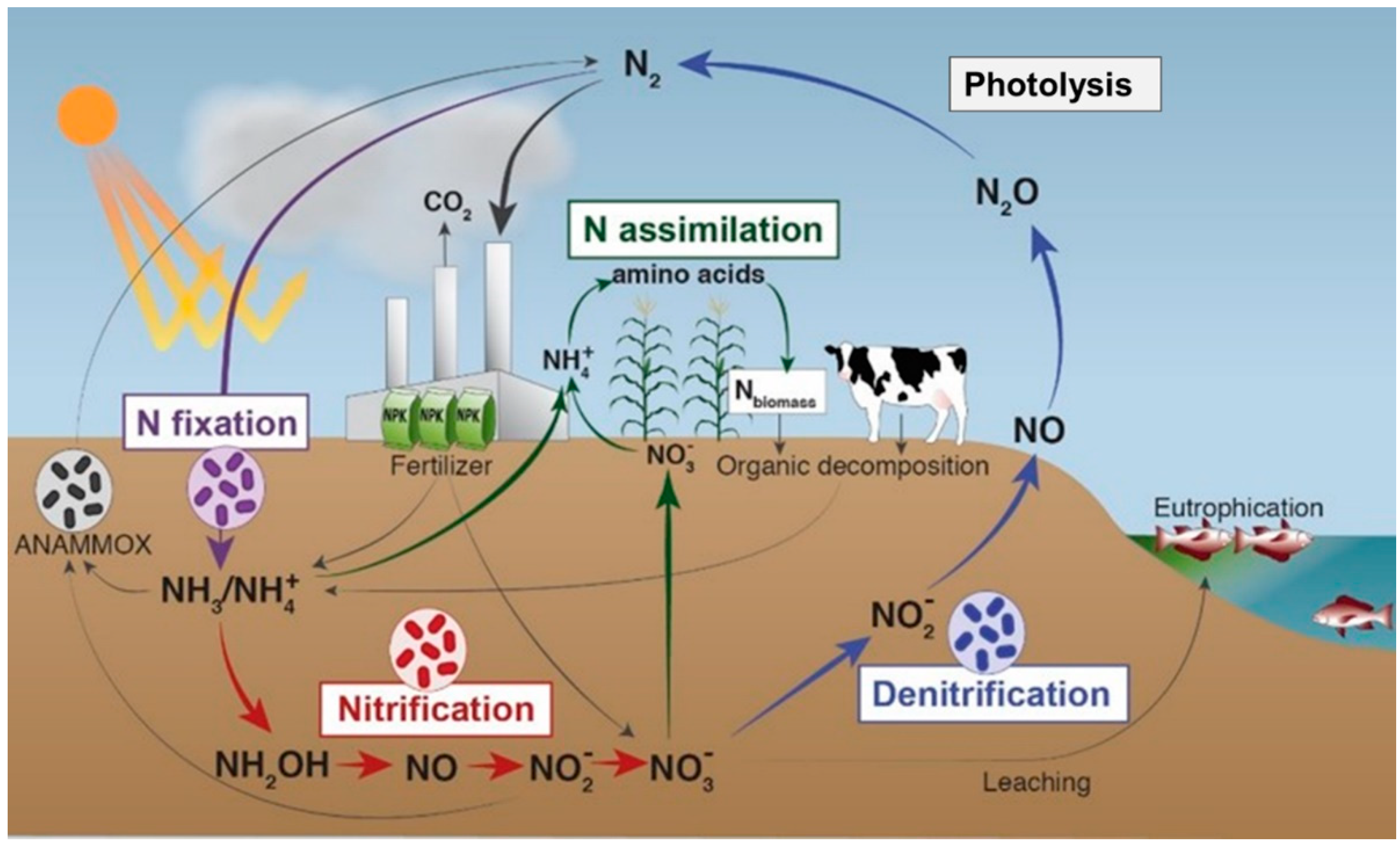
2. Sources and Sinks of N2O

N2O gas is a natural byproduct of the nitrogen cycle, which is one of the most important biogeochemical cycles in the world. The nitrogen cycle starts with the fixation of dinitrogen (N2) gas, which comprises 78% of our atmosphere, into ammonia (NH3) and ammonium (NH4+) in the lithosphere [5]. The conversion of nitrogen into other forms can be mediated by microbes [6], leguminous crops [7] and/or natural processes like lightning [8]. A synthetic fixation is also possible through the Haber–Bosch process, which has established its dominance over the natural fixation [9,10,11]. However, the majority of plants and autotrophs cannot use the abovementioned forms of nitrogen directly for their basic processes. They can uptake nitrogen as nitrates (NO3), which are rather unstable and easily susceptible to drainage and leaching [12].
The oxidation process under favorable conditions can convert NH3 and NH4+ into nitrites (NO2) and finally into nitrates (NO3), a process which is known as nitrification. The conversion process is facilitated by chemoautotrophic bacteria (e.g., Nitrosomonas, Nitrosospira and Nitrosolobus [13]) under favorable environmental conditions, including sufficient aeration (e.g., Jamieson et al. [14] showed 93% removal of ammonia via nitrification when aeration was introduced in a soil system, compared to 50% removal efficiency in non-aerated conditions), NH4+ concentrations, soil temperature (nitrification is reported to be at maximum around 20–25 °C [15]), suitable pH levels (nitrification is reported to linearly increase with soil pH ranging from 4.9 to 7.2 [16])) and others. Intermediate products like hydroxylamine (NH2OH), nitric oxide (NO) and nitrous oxide (N2O) also form during the nitrification process [17,18]. A direct contribution of N2O may also come from oxidation of NH2OH, known as “nitrifier denitrification” [19], or an indirect production which may arise from transported nitrogen via volatilization, deposition, leaching and runoff [6]. These gases, in the form of NO and N2O, are released back to the atmosphere and are a potent source of global warming.
N2O and NO are also released during the denitrification process of a nitrogen cycle when unstable NO3 and NO2 convert to more stable dinitrogen [20]. During this reductive process of denitrification, a certain fraction of gases is also released in the form of N2O. This process is also facilitated by facultative microbes (denitrifiers, e.g., Pseudomonas, Alcaligenes and others [21]), which can reduce NO3 and NO2 to N2O and N2 under anaerobic conditions, abundant soil nitrates, soil organic content (SOC), higher soil temperatures, neutral to slightly basic soil pH (pH above 7 leads to higher N2:N2O ratio [22]) and higher water-filled pore spaces (WFPS) (WFPS more than 60% [23]).
The dominant source of N2O emission may be either nitrification or denitrification, depending on the soil properties, including water-filled pore spaces (e.g., during 35%–60%, nitrification dominates, while above 60%, denitrification is a major source of N2O flux [23]), oxygen concentration, nitrogen and residue (as carbon source) availability and others [24,25].
Unlike sources, sinks (where N2O is converted to other products that are less harmful and thus has a negative effect on radiative forcing) are not straightforward for N2O. In the atmosphere, N2O may be removed by photolysis with ultraviolet light [3], but it takes a very long time. However, N2O reduction strategies could be adopted following schemes proposed by Schlesinger [26] and Bakken and Frostegård [27]. The scheme includes minimization of N2O:N2 product ratio, N2O:N2 ratio of denitrification and anammox (anaerobic ammonium oxidation), N2O:NO3 ratio of nitrification, and N2O:NH4+ ratio of dissimilatory nitrate reduction to ammonia in systems like agricultural soils, managed wetlands and wastewater treatment plants. A simple N-cycle showing sinks and sources of N2O based on above discussions is adapted from Lehnert et al. [28] and is presented in Figure 1.
While N2O emissions may arise from different systems, like riverine, livestock rearing and even commercial products, the focus of this article is on agricultural emissions, since they account for most of the anthropogenic emissions (around 67%–80%), as reported by Wrage et al. [29] and Ussiri and Lal [30].

3. N2O Controlling Factors

In this study, factors affecting agricultural N2O emissions are divided into three groups: environment-related, crop-related and management-related.

3.1. Environmental Factors

3.1.1. Weather

N2O emissions from arable lands are dependent on weather variables like rainfall [31] and temperature [32] and vary with seasonal [33] and weather patterns [34]. The effect of weather variables is already significant, and when compounded with other variables, like crop type, residue and management, N2O emissions are significantly altered [31]. High rainfall can lead to high soil moisture and favor denitrification conditions, and this can lead to high N2O emissions. Thus, rainfall events can trigger pulse N2O emissions. Moreover, seasonal characteristics may enhance the impact of rainfall-induced emissions [35]. Pulse N2O emission may be defined as value(s) greater than twice the standard deviation of the moving average (emissions with 90-day moving window) and is neighbored by at least one similar other value [36]. Such pulses may be few in number (not to be confused with outliers), but contribute a significant amount (20%–80%) of the total emission [36]. Air temperatures also impact seasonal N2O emission patterns, especially due to increased microbial activities during nitrification and denitrification [37]. Hot–humid seasons have been attributed with higher emissions than cold–dry season for different land use in China [33]. Weather patterns have also been found to correlate with temporal variability of N2O emissions driven by nitrogen mineralization rates in different counties in the USA [34].

3.1.2. Freeze–Thaw Cycles

In high-altitude or -latitude regions, freezing and thawing of soil is a seasonal process and affects the vertical and horizontal movement of moisture and nutrients. Soils with higher water content are prone to freezing than soils with lower water, even at same temperature [38]. The freezing-and-thawing processes are known to alter soil’s physical properties, microbial biomass and nutrient distribution, along with causing a general increase in denitrification upon thawing [39]. The alternate freezing and thawing of soils in cold climatic regions also leads to pulse N2O emissions [40]. This enhanced release could be due to the physical release of trapped N2O from underneath the frozen layers or due to the immediate production at the onset of thaw from increased biological activity. Failure to account for the contribution of N2O from freeze–thaw cycle is expected to underestimate global agricultural N2O emissions by 17%–28% [41].

3.2. Land- and Crop-Management Factors

Land uses have impacts on N2O emission patterns [33]. For agricultural lands, vegetable lands were reported to have higher emissions than orchards and uplands (having crops like corn, peanut, sweet potato, and chestnut interplanted with Camellia sinensis and rapeseeds) [33]. Emissions from grasslands may be higher than that from arable soils [42]. However, such emissions may not increase significantly, compared to their arable counterparts, under increasing water-filled pore spaces. The emissions may even diminish with increasing water-filled pore spaces for restored lands, such as prairie lands [35]. The higher emissions of N2O from grasslands are reported by Schaufler et al. [43] compared to croplands, forests and wetlands because of the presence of high soil microbial activity stimulated by higher carbon and nitrogen contents. Vilain et al. [44] reported that riparian buffers, followed by grassland had higher N2O-emission potential than forests. Even for the same land use, the fluxes may differ, depending on their previous land-use history [45]. Katulanda [46] discussed the effect of legacy land use and how they affect the microbial communities and regulate nitrogen cycle, even after a long time. Studies have also shown that animal grazing could accelerate N2O emission [47,48].
Similarly, different crop-management practices can alter biogeochemical cycles, the understanding of which is crucial for greenhouse-gas-emission modeling. A meta-analysis by Mei et al. [49], based on 40 peer-reviewed publications, suggested that N2O fluxes are more affected by crop-management practices than the soil properties.

3.2.1. Tillage

Tillage changes the soil structure and redistributes soil minerals and is thus expected to impact GHG processes. No-till and reduced tillage (both are subsets of conservation tillage) have been reported to yield higher N2O fluxes from agricultural lands compared to conventional tillage [50,51]. Though conservation tillage has been considered to be a potential mitigation option for CO2 emissions due to the enhanced soil carbon sequestration, it is likely to increase N2O emissions compared to the conventional tillage [49] and thus limits its benefits. This may be due to the better aeration and diffusivity of gases in case of conventional tillage, compared to best management practices, like no-till and the cumulative impact of residue accumulation. Kessel et al. [50] reported that the effects of tillage were more complicated based on a meta-analysis of 239 comparative studies. On average, there was no significant variation in N2O fluxes between conservation and conventional tillage [52]. They also reported that, in dry climates, conservation tillage increased N2O fluxes significantly (57%) when practiced for less than 10 years but decreased significantly (27%) afterward. N2O fluxes were also reported as being high in soils with perennial crops, compared to those with annual crops, possibly because of the minimum requirement of tillage [53].

3.2.2. Fertilizers

Nitrogenous fertilizers are often reported as the single best predictor and proxy of N2O fluxes from agricultural soils [54,55] and have a positive relationship [33]. Shcherbak et al. [54] also reported that the response of N2O to increasing nitrogen fertilizer use is not linear as IPCC suggested, but an exponential one. Whenever nitrogen fertilizer application exceed crop requirement, the emissions of N2O were significant [54]. Fertilizers enrich the arable lands with ammonium and nitrates, which are eventually taken by plants and/or leached, washed off or lost as gases [56]. They regulate farm processes and increase crop yields. However, their introduction into the nitrogen cycle increases N2O fluxes, especially during wet seasons [57]. These increased emissions are short-lived and have been found to drop back to normal levels within 2–6 days, depending on a number of factors [58,59]. Moreover, N2O emissions from nitrate-based fertilizer are reported to be significantly higher than those from ammonium-based fertilizer, under wet conditions [60]. The application technique and depth of fertilizer-N application are also reported to alter the N2O fluxes [52]. Enhanced nitrogen fertilizers, which are formulated to reduce nitrogenous losses to the environment by preventing NH3 volatilization and by inhibiting urease activity and nitrification, can reduce nitrification/denitrification losses and thus the N2O emissions from agricultural systems [61,62]. Improvement in fertilizer application and management techniques have been known to reduce the annual nitrogen fertilization rates, irrigation requirement and increase the crop production with significant decrease in N2O emissions [33]. Practices such as split fertilizer application and the use of the recommended fertilizer dose can significantly (20%) reduce N2O emission [63].

3.2.3. Residues

Residue incorporation increases greenhouse gases’ fluxes from arable lands. Long-term incorporation of residues are known to significantly increase such fluxes [64]. Likewise, management of residues, like stover removal, reduces the N2O emission [61,64]. Leaving leguminous-crop residues in fields contributes excess nitrogen and leads to higher emissions than the grass residues [65]. Introducing biochar, however, may decrease such fluxes, without decreasing the yields [66].

3.2.4. Cover Crops

Cover crops are planted for their several inherent environmental benefits [67]. However, their reported effects on N2O emissions are ambiguous, with 60% of studies indicating an increase, and remaining studies indicating a decrease [68]. Crops which can fix nitrogen (leguminous crops) are likely to increase such fluxes more than other crops [54]. Cover crops may benefit by up-taking soil nitrates, but they might add more mineralizable carbon and could emit more N2O [69]. The presence of leguminous residue is likely to increase N2O emissions from the nitrification, compared to denitrification, process [24].

3.3. Soil Characteristics

3.3.1. Soil Type

Soil type not only affects the magnitudes of emissions, but also their patterns. For example, clay soil has been reported to have higher N2O fluxes compared to sandy clay loam and loess for the same moisture content in several studies, which is due to the higher soil organic carbon and mineral levels in clay soils [53,70]. Similarly, Xiong et al. [70], reported higher N2O emissions in clay soils during non-flooding to flooding period and in loess soil during flooding to non-flooding period. In general, however, soils with finer texture are reported to have higher N2O emissions than the coarser ones, as they retain higher soil moisture, are more compact in nature and have localized high microbial activity [71,72].

3.3.2. Soil Temperature

Several studies have described the relationship of N2O emissions and soil temperature as exponential [73]. N2O emissions are widely known to increase with increasing soil temperature, with peak values around 20–35 °C (Parton et al., 2001). However, these peak temperature values may vary from region to region, based on their climatology and adaptability of micro-organisms, along with the presence of other organisms, like earthworms [74,75]. For example, N2O fluxes were negligible from soils when temperature dropped below 5 °C, started to increase till it reached 20 °C and decreased again with increasing temperature in Hungarian loess soil [76].

3.3.3. Water-Filled Pore Spaces

Water-filled pore space (WFPS) is another key factor controlling N2O fluxes from agricultural soils. Microbiological denitrification is reported to occur when WFPS is in the range of 65%–80%, generally following intense rainfall events [65,77,78,79]. N2O is found to be positively correlated with soil moisture [43], and its previous legacies (historical land use) [78]. For different soils, the range of optimal WFPS for maximum N2O production is also different.

3.3.4. Compaction

Compact soil means less aeration, which alters gas diffusivity and increases N2O fluxes from favorable denitrification conditions [80]. For example, Tullberg et al. [81] reported double emission from a trafficked soil compared to non-trafficked one. Ball et al. [82] explained how trampling of urine rich fields reduced air permeability and pore continuity, without changing the bulk density, increased cumulative N2O emissions significantly. Ball et al. [82] also explained how the trampling did not impact the performance of inhibitors and was successful in decreasing N2O fluxes when used. Implementation of biochar is reported to alleviate the impacts of soil compaction on crop growth and mitigate N2O fluxes [83].

3.3.5. Carbon and Nitrogen

Increasing soil organic carbon (SOC) content is reported to increase N2O fluxes differently for different soil types [71]. The N2O emissions were reported minimal when the mineral nitrogen in the top soil layer (0–15 cm) was less than 20 mg N/kg in Canadian soils [84]. N2O emissions also showed a significantly positive correlation with mineral nitrogen present in sugarcane fields in Australia [85]. The ratio of carbon content to the nitrogen content available in soil has also been identified as an efficient index to estimate N2O emissions, when cover crops are used [65]. The soils with low C:N ratio and high N content can accelerate N mineralization and, thus, higher N2O emissions, while the soils with reverse characteristics can have less impact on emissions [86].

3.3.6. The pH

The pH controls N2O emissions by affecting different enzyme activities [87]. For example, Liu et al. [88] reported low fluxes at neutral to basic pH for most of the soils. Wagena et al. [89] also reported that, although total denitrification increased, the total emissions reduced by 70%–74% at a soil pH of 8 compared to a pH of 6.5 when N2O fluxes were simulated in the USA. Similarly, pH values in the range of 4–8 are expected to increase the N2O:N2 ratio. At a pH value below 4, denitrification gets inhibited [88].
While all these factors are responsible for N2O emission, the interaction among them to supply readily available substrates of nitrogen is also equally important, if not more.

4. Capability of Process-Based Models for N2O Emission Modeling

Theoretically, any model capable of simulating a nitrogen cycle may be used to estimate nitrate (NO3) leaching, nitrous oxide (N2O) emissions and ammonia (NH3) volatilization [90]. Denitrification-Decomposition (DNDC [91]), CENTURY [92], daily CENTURY (DAYCENT [93]), modified Nitrate Leaching and Economic Analysis Package (NLEAP [94]), Expert-N [95], ecosys [96] and root zone water quality model (RZWMQ [97]) are some of the process-based models that are capable of estimating N2O emissions and have been extensively tested in agricultural systems. However, modelers agree that modeling such fluxes from soil is quite vexing due to the interaction of different biotic and abiotic factors and processes (e.g., nitrification and denitrification), many of which are still not fully understood [98]. Chen et al. [99] reviewed multiple laboratories’ field-, regional- and global-scale N2O emission models and reported that, while all models have their own unique limitation and strengths, the majority of modelers prefer robust field-scale models that can be upscaled. The primary challenges in efficient N2O modeling, as discussed by Chen et al. [99], included uncertainties arising from limited temporal resolution of experimental data, identification of N2O contribution from nitrification and denitrification processes, partition of N2O:N2 during denitrification, development of N2O emissions from chemo- and nitrifier-denitrification and analysis of N2O diffusion from depth and profile of soil and have been repeatedly raised by successive studies including Zhang et al. [100], Regaert et al. [101] and Gaillard et al. [102], among many others.
Since N2O fluxes are affected by several factors and their interaction components, a process-based model that can incorporate all of these components is needed for realistic simulations. The model should have robust components of hydrology, nutrient management, crop, land use and management practices, to include all possible facets of N2O emission. Ehrhardt et al. [103] assessed the ability of 24 process-based biogeochemical models for N2O emission modeling from wheat, rice, corn and temperate grasslands for blind, partial- and full-calibration scenarios and reported that, even with full calibration, the errors in N2O emissions did not reduce significantly, compared to blind or partial scenarios. Furthermore, most of the aforementioned models and those used by Ehrhardt et al. [103], in principle, consider only the vertical transfer of hydrologically driven nutrient transport, while lateral transfer of nutrient is important in watershed scale [104]. Among few potential models, the Soil and Water Assessment Tool (SWAT) [105] is becoming increasingly popular among ecological modelers, to estimate N2O emissions at the watershed scale.

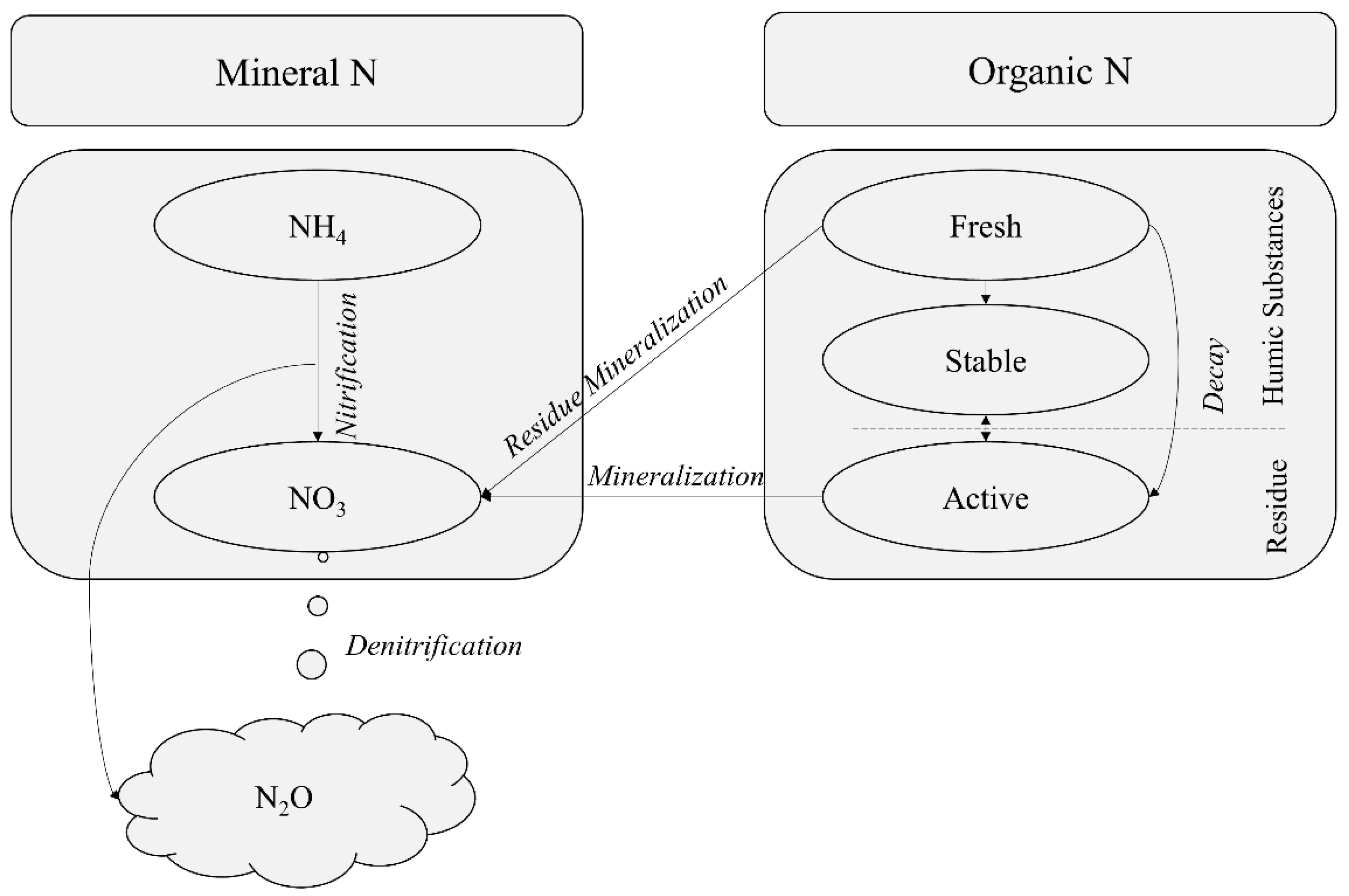
5. Introduction to SWAT

SWAT is a process-based, continuous hydrological model which was initially developed to assist management of water-resources system and non-point sources of pollution in large river basins [106]. Over the years, it has been extensively tested in multiple river basins across the globe and has been reported to replicate their quantitative and qualitative aspects satisfactorily [107,108]. A brief history of SWAT development can be found in Williams et al. [109]. The advances in SWAT modeling since the last decade include development of user-friendly GIS interface; inclusion and assessment of potential impacts of sediment loading, nutrients and best management practices; ponding and wetlands; climate change; water-resources management; and groundwater and biogeochemical cycles [105,110,111,112,113,114,115].
Among different biogeochemical cycles included in SWAT, the nitrogen cycle (N-cycle) module is the one responsible for N2O emissions. A typical model layout of SWAT simulating the N-cycle and N2O emission is presented in Figure 2.
The details on how SWAT conceptualizes nitrogen cycle can be referred from the Supplementary Materials section of this article. It can also be referred from theoretical documentation of SWAT [114]. As such, the most recent version of SWAT (SWAT2012 rev. 670) incorporates nitrification and denitrification components in its N-cycle but does not explicitly quantify the N2O emission during the processes. Gramig et al. [116] reported that, until 2012, none of the hydrological models including SWAT could simulate biogeochemical cycles. Thus, various researchers have developed or integrated several N2O simulation modules in SWAT, for different regions, in the recent years.

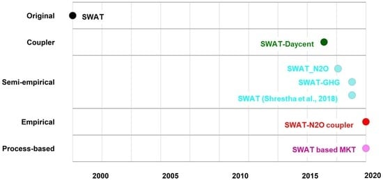
6. Advancements of SWAT in Simulating N2O Emissions

The updates of N2O emission modules in SWAT are categorized into coupler, semi-empirical, empirical and process-based revisions. Coupler revisions include integration (simultaneous) of SWAT with another biogeochemical model, using an independent platform like OpenMI. The outputs of one are used as input for the other model, to derive final integrated outputs. Semi-empirical revision means inclusion of established semi-empirical equations of nitrification and denitrification within SWAT. Empirical revisions mean inclusion of an empirical equation within SWAT, which is specific to an area or a region and does not explicitly split nitrification and denitrification schemes. These equations give cumulative N2O emissions, using different SWAT variables. Process-based revision means the inclusion of a detailed oxidation-reduction-potential model, which quantifies emission of N2O under different states in SWAT. A brief development history of such revisions is presented in Figure 3 and subsequently explained in the sections below.
There have been several modifications made to the SWAT hydrological model, as reported by several researchers, since its development in 1998. However, Figure 3 shows the timeline of the first version of SWAT and not its revisions. Moreover, the application of the N2O emission models using the modified SWAT models are also not reported. It only reports the development and modification of SWAT for N2O emission modeling. Moreover, the year attributed to the development is the year when the corresponding research article was accepted for publication in a peer-reviewed journal. It is distinctly visible that the developments have picked a rapid trend since 2016, with the majority of research being on semi-empirical revisions of SWAT.

6.1. Coupler Revisions

The first framework to integrate SWAT and DAYCENT was developed by Reeling and Gramig [117] and included a genetic algorithm to analyze the optimal conservation practices, but the integration was not simultaneous (it used both models separately). The first-ever simultaneous N2O emission module in SWAT was added by Wu et al. [114], who developed DAYCENT input files for each hydrologic response unit (HRU) and drove DAYCENT automatically (coupler named SWAT–DayCent). SWAT was chosen as the base model to integrate DAYCENT because of its easy-to-setup-and-use configuration and its availability of user interface for spatial analysis. There was no need of separate inputs for DAYCENT once the modeler developed a SWAT project for his region of interest. Specifically, the authors obtained SWAT HRU variables, like soil properties, site-specific properties, daily weather data, management data and other data. They then wrote them into input files for DAYCENT and used a loop to run DAYCENT at each unit and aggregated the output files. This allowed modelers to analyze the DAYCENT outputs at the same spatial details of the watershed, in addition to typical SWAT outputs.
The discrepancies in SWAT’s original output structure at HRU and input data structure of DAYCENT were addressed in the coupler by adding input files on detailed soil structure and property information, long-term weather statistics, daily weather and land management information at the HRU level [114]. The authors discussed that the watershed delineation and configuration of HRU affected not only SWAT, but also the DAYCENT simulation results. The major biogeochemical outputs of SWAT–DayCent were net primary production (NPP), soil organic carbon (SOC), biomass, yield, soil respiration and N2O fluxes. These outputs were then aggregated with SWAT outputs, to provide comprehensive simulation results of hydrological and biogeochemical cycle modeling.
SWAT–DayCent was later used by Zhao et al. [118] in the semiarid upper Wei River Basin of China, where the authors used remotely sensed NPP values to calibrate the DAYCENT component. Zhao et al. [118] identified “PRDX” (potential tree/grass/crop/aboveground production) as the sensitive parameter for SWAT–DayCent model. However, it is worthwhile to note that “PRDX” may be subjected to easy overfitting, while aiming the calibration of such models. Performance of the coupler was satisfactory in simulating hydro-biogeochemical cycles (annual R2 values ranged from 0.36 to 0.63, and bias was less than 2%) in not only the Wei River, but also in the Jhinge River Basin of China (annual R2 value ranged from 0.25 to 0.83, and bias was less than 15%) [118,119]. Though N2O fluxes were not simulated and validated with the coupler in these studies, it showed the potential to satisfactorily estimate N2O fluxes from agricultural watersheds. With increasing availability and accessibility of open-access platforms like Open Modeling Interface (OpenMI), couplers like SWAT–DayCent can be implemented in full fledge [120].

6.2. Semi-Empirical Revisions

Yang et al. [121] integrated N2O emission algorithm of DAYCENT (semi-empirical equations of Parton et al. [122]) with the nitrogen cycle of SWAT (modified version named SWAT–N2O) and tested the model for three agricultural systems with different management intensities in Southwestern Michigan, USA. The default parametrization of SWAT–N2O had satisfactory reproduction of N2O emission from corn, switchgrass and smooth brome grass sites, and the model performance was further improved when the parameters were calibrated. The equations used by SWAT–N2O for nitrification and denitrification N2O are presented below:
Nnit = fmoist * fst * fpH * Nnit_max + Nnit_base
fmoist = 1/(1 + 30 * e^(−9*relwc))
relwc = (SW/STH−SWmin)/(FC/STH−SWmin)
SWmin = WP/STH − SWdel
fst = e^((4.5*(5*ST/(−40))^7*(5*ST/(−40))^4.5))/7)
fpH = 0.56 + 1/π *atan(π* 0.45 * (SPH−5))
Nnit_max = fnit_max*NH4
where Nnit is the soil nitrification rate, estimated using maximum (Nnit_max) and minimum (Nnit_base) nitrification rates, maximum fraction of ammonia nitrified during nitrification (fnit_max), soil water content (SW), temperature (ST), depth, pH (SPH), ammonium content (NH4) and moisture at wilting point (WP) and field capacity (FC), minimum soil water content (SWmin) and minimum volumetric soil water content below wilting point (SWdel).
N2O production from nitrification (EN2O_nit) was specified as a fraction of nitrified ammonia as follows:
EN2O_nit = fN2O_to_nit*Nnit
fN2O_to_nit = (adjwp−adjFC)/(dDOwp−dDOFC) * (dDOsf−dDOwp) + adjwp
where, fN2O_to_nit = maximum ratio of N2O production to nitrified nitrogen at field capacity, minimum ratio of N2O production to nitrified ammonia at wilting point, normalized diffusivity of soil at field capacity and wilting points, and normalized diffusivity of the topsoil layer.
Similarly, Yang et al. [121] revised the denitrification algorithm in SWAT–N2O, following Parton et al. [122] and Del Grosso et al. [123]. N2O emissions from denitrification (EN2O_den) were estimated as a function of denitrification rate (Eden), ratio of N2:N2O (Rn2n2o), CO2 effect on N2:N2O (fRno3_co2), WFPS effect on N2:N2O (fRwfps), normalized soil diffusivity (fDOfc), soil nitrate content (nppm), soil carbon dioxide content (co2ppm), denitrified nitrogen (Dtotflux), effects of WFPS on denitrification (fDwfps), soil density (ρsoil), denitrification rate due to CO2 concentration (fDco2), denitrification rate due to soil nitrate (fDno3), minimum nitrate concentration in a soil layer for trace gas calculation (min_nit), impacts of CO2 concentration on fDwfps (x-inflection) and soil respiration (respc), as presented in the equations below:
EN2O_den = Eden/(1 + Rn2n2o)
Rn2n2o = fRno3−co2 * fRwfps
fRno3−co2 = (38.4−350*dDOfc) *e^(0.8*nppm/co2ppm)
fRwfps = 1.5*wfps − 0.32
ENden = Dtotflux * fDwfps * Cunit * ρsoil
Dtotflux = min(fDco2,fDno3)
fDco2 = 0.1 * (CO2correction)1.3minnit
fDno3 = 1.556 + 79.92/3.14 * Arctan(3.14 * 0.0022 * (nppm−9.23))
fDwfps = (0.45 + (atan(0.6 * π * 10 * (wfpsxinflection))))/π
wfps = swcfrac/porosity
xinflection = (9 − M*CO2correction) *wfpsadj
M = dDOFC*(−1.25) + 0.145
CO2correction = CO2ppm * (1 + aa*(wfps−wfpsthreshold))
CO2ppm = respc/ρsoil
where cunit is a conversion coefficient to change from ppm to g/g, co2correction is corrected CO2 concentration, M is a parameter to calculate x-inflection, aa is impact of soil diffusivity on soil CO2 concentrations, wfpsthreshold is a threshold value for wfps and wfps_adj is the correction factor in inflection point for wfps effect on denitrification curve.
In general, the variability (explained by R2) of N2O fluxes simulated by SWAT–N2O were reported around 22% by Yang et al. [121] for emissions, including extremely high values and around 49% when such extremes were excluded. Parameters like adjustment on inflection point for WFPS effect on denitrification curve, maximum fraction of N2O to nitrified nitrogen at field capacity and maximum fraction of ammonia nitrified during nitrification were reported sensitive in N2O emissions. The highest sensitivity of adjustment on inflection point for WFPS effect on denitrification curve represents the soil properties affecting soil diffusivity along with moisture, texture and density for which better datasets and algorithms are needed to define the underlying mechanisms. The high fluxes of N2O, especially after fertilizer use, were reported to highly impact the model’s performance, for which finer temporal measurements were recommended by Yang et al. [121]. A more comprehensive parameter optimization algorithm was also recommended, and the cumulative sensitivity of the model parameters were suggested for future research.
A few of these suggestions have been incorporated by Wagena et al. [89] in modifying SWAT–VSA (integrated model termed SWAT–GHG) to estimate N2O emissions from agricultural plots of USA. SWAT–VSA is a reconceptualization of SWAT to account the areas where saturation dynamics is variable in nature [124] and is thus an advancement in simulating hotspots of N2O fluxes. Wagena et al. [89] used the denitrification flux equation of Parton et al. [125] and Mosier et al. [126], which is similar to the revised model of Yang et al. [121]. However, the authors used an additional variable, the pH, in estimating total denitrification rate (DNtotal), as follows:
DNtotal = min[Fd(NO3),Fd(C)]*Fd(θ)*Fd(T)*Fd(pH)
where, Fd(NO3), Fd(C), Fd(ϴ) and Fd(T) are similar to that of Equations (32) and (33). The Fd (pH) was calculated as follows:
Fd(pH) = {(0.001 for pH ≤ 3.5; (pH-3.5)/3 for 3.5 < pH < 6.5; 1 for pH ≥ 6.5)}
Similarly, the N2O emission from nitrification process included the same empirical equations of Parton et al. [93] and Parton et al. [122], but also incorporated effects of pH as follows:
FN2O = FNO3 * K2 * Fθ * Ftemp * FpH
FpH = 0.56 + (arctan(π*0.45*(soilpH-5)))/π
SWAT–GHG was reported capable of capturing N2O fluxes from agricultural watersheds of Indiana and Pennsylvania. The model performance statistics R2, calculated from the discrete observations and simulations indicated a good model performance in N2O emission simulation in the range of 0.5–0.95 during calibration and 0.4–0.7 during validation. The identified sensitive parameters in SWAT–GHG were soil pH and N, followed by soil temperature, moisture and carbon levels. SWAT–GHG was used by Wagena et al. [127] to analyze the impacts of climate change on N2O fluxes. Changing soil moistures under future conditions were reported to alter the emissions from soils by Wagena et al. [127]. A combination of modules reported by Yang et al. [121] and Wagena et al. [89] was done by Shrestha et al. [47] with minor modifications, to estimate N2O fluxes from long-term grasslands in Canada.
Shrestha et al. [47] also incorporated semi-empirical equations of nitrification and denitrification modules suggested by Parton et al. [125] and Parton et al. [122] into SWAT. The estimation of N2O from denitrification was done using the same partitioning approach of Equation (10). However, a temperature reduction factor was complemented in addition to that of Yang et al. [121], and the pH factor was neglected from Wagena et al. [89], explaining that up to 95% of N2O dynamics from denitrification are explained by variations in soil moisture and temperature [47]. The total denitrification calculated by the model of Shrestha et al. [47] can be represented as follows:
DENITtotal = min[Fdenit,NO3, Fdenit,C] * Fdenit,wfps* Fdenit,solt
Fdenit,solt = max[(0.9*Tsoil/(Tsoil + e^(9.93−0.312*Tsoil)) + 0.1),0.1]
The contribution of N2O from nitrification was also taken from established equations of Parton et al. [125], as opposed to Wagena et al. [89], who took SWAT’s original formulation. The fraction of nitrogen was taken as a calibration parameter. While the remaining explanation of the variables could be referred to Shrestha et al. [47], the equations are fairly similar to that of Yang et al. [121]. Shrestha et al. [47] replicated the discrete N2O measurements in the range of 0.02–0.47. The model developed by Shrestha et al. [47] was used by Melaku et al. [59] to estimate N2O emissions from selected grassland sites of the United Kingdom applied with solid manure and had good performance (R2 values of 0.58–0.71 for discrete measurements) in representing the dynamics of fluxes.
While all models discussed above included only direct emissions (occurring within the soil), Fu et al. [128] developed both direct and indirect (occurring from streams) N2O emission modules in SWAT. Fu et al. [128] also developed a calibration module to estimate spatiotemporal flux of direct and indirect emissions and tested it in different order of streams and catchments in Minnesota, USA. Direct emission modules were integrated with SWAT’s nitrogen cycle, while indirect emissions were calculated from SWAT’s stream transportation of nitrates. The nitrogen cycle adopted in the model of Fu et al. [128] was that of the Century model [129] and is thus similar to the above mentioned models. The direct N2O emissions can be calculated by using the parameters from Community Land Model version 4.5 by Fu et al. [128], as follows:
EN2O_nit = 6* 10−4 *Nnit
where EN2O_nit = N2O emissions from nitrification and Nnit = nitrification rate.
Similarly, the ratio of N2:N2O (PN2:N2O) by denitrification was calculated by following Del Grosso et al. [123]:
PN2:N2O = max(0.16*k1,k1*e^(−0.8*PNO3:CO2))*fWFPS
fWFPS = max(0.1, 0.015*WFPS−0.32)
where PNO3:CO2 = ratio of CO2 production/soil respiration to nitrate concentration in soil, K1 = calibration parameter affected by soil gas diffusivity and fWFPS = function of water-filled pore space (WFPS).
The indirect emissions of N2O from the streams once nitrates are transported are calculated as a function of surface water N2O concentration, equilibrium N2O concentration and N2O transfer velocity as follows:
F = k*(N2O−N2Oamb) * 413.2
where F is N2O emission from unit water surface area, k is N2O transfer velocity, N2O is the surface N2O concentration and N2Oamb is theoretical N2O concentration in equilibrium with atmospheric N2O.

6.3. Empirical Revisions

A few researchers have developed modules to simulate N2O emission from agricultural farms by using equations derived from observed data and integrating them with SWAT. Gao et al. [130] for example, used 4488 measurements of N2O emissions and other soil variables and developed empirical equations for N2O fluxes. However, there is no partitioning between nitrification and denitrification. The modified SWAT model of Gao et al. [130] was named SWAT–N2O coupler and it could simulate N2O emissions from soils in paddy and non-paddy fields at different spatiotemporal scales. Different variables established in the literature and known to be sensitive on N2O emissions, like soil nitrate, temperature, moisture, etc., were used to define the fluxes from different agricultural scenarios. For non-paddy fields, Gao et al. [130] integrated the following equation in SWAT:
N2Osoil = −6.519 + 1.075*SN + 0.246*ST + 0.12*SW
where N2Osoil = emission fluxes, SN = soil nitrate, ST = soil temperature and SW = soil water content in the soil layer.
For paddy fields, the base SWAT model was not the unaltered one, but the revised version developed by Xie and Cui [131], where different irrigation modes for paddy were defined. N2O emission algorithms for different irrigation modes were integrated into the SWAT model as follows:
N2Opaddy = −0.249*(SN)2 + 14.448*ln(ST) − 31.909 for control irrigation
N2Opaddy = −0.228*(SN)2 + 6.561*ln(ST) − 9.463 for intermittent irrigation
N2Opaddy = −0.616 * ln(SN) + 0.011*(ST)2 + 5.191 for basin irrigation
The SWAT–N2O coupler is also reported to provide modelers the features of spatiotemporal analysis, sensitivity and scenario analysis module and was tested in agricultural fields of Northeast China [130]. The study demonstrated the capability of the model to simulate N2O hotspots under different land uses and also reported its sensitivity to precipitation in non-paddy fields and temperature in paddy fields. The coupling was reported to be more precise compared to the previous versions and could explain 52%–78% of variability (R2 for discrete measurements of N2O for different soil NO3 levels) of N2O fluxes in the study area. The fluxes increase under the scenarios of increasing nitrogen application rates and may decrease under a warmer and wetter climate in paddy fields and increase under a warmer and drier climate in non-paddy fields.

6.4. Process-Based Revisions

While the majority of the aforementioned studies used semi-empirical and empirical equations, very few researchers have used mechanistic approach in estimating N2O emissions using SWAT. A detailed decomposition process of soil organic matter based on Microbial Kinetics and Thermodynamics (MKT model) was integrated with the SWAT model by Bhanja et al. [132]. Sequential oxidation reduction potential and chemical reactions were formulated at the soil–water zone, using dual Michaelis–Menten kinetics, for which the required variables were taken from SWAT. A testing of the developed model for three different locations in Saskatchewan, Canada, showed improved performance in N2O emission estimations, compared to other modified SWAT models discussed above. The R2 values computed by using discrete measurements of N2O and model simulation showed that the model was able to explain 40%–80% of the variability in the fluxes.

7. Limitations

While all coupled, empirical, semi-empirical and process-based revisions of SWAT are dedicated to estimate N2O fluxes from agricultural watersheds, all models have some limitations. The performance of these models is not able to adequately explain the variability of fluxes, often ranging from R2 values of 0.52–0.78 at monthly timestep and 0.0–0.6 at daily timestep [47,130]. However, the DAYCENT model itself was not able to capture the daily emissions satisfactorily in its initial application [122]. Therefore, it maybe overambitious to apply SWAT to simulate daily N2O flux satisfactorily. N2O processes are highly temporal in nature and often vary significantly during sub-daily resolutions, which is yet to be established in SWAT (as its lowest simulation time-interval is daily).
Currently, none of above-discussed models incorporated freeze–thaw cycle module, which is a characteristic process in cold regions, and thus the associated pulse N2O fluxes are overlooked. As discussed by Wagner-Riddle et al. [41], such processes may contribute significant amounts of emissions. The landscape effect, which has prominence in biogeochemical models, was incorporated into SWAT by using its VSA modified version, but the use of static pH has limited its full potential [89]. A dynamic pH inclusion in the model can simulate impacts of different management practices, like liming or acid fertilization on N2O emissions.
Calibration components in these models were mostly manual [89,121]. Moreover, these models were not able to calibrate the contribution of nitrification and denitrification separately, which needed to be addressed, mostly from the observation standpoint. The timing of N2O peaks is also quite difficult to model due to the discrepancies in measured and simulated temporal resolutions. Moreover, several environmental variables affecting N2O fluxes are very difficult to measure and will miss their spatial and temporal characterization in modeling [104].
While process-based algorithms and techniques may be expected to yield better results than semi-empirical and empirical approaches, such techniques are relatively complex, and the data required to support them might not be readily available. The bi-directional nature of nitrogen release and deposition and their impact on ecosystem [133] are yet to be integrated into SWAT. Furthermore, the existing structure of SWAT itself may be not supportive enough for fully process-based biogeochemical model.

8. Recommendation

So far, the integration of SWAT has been done with either DAYCENT or with semi-empirical equations included in DAYCENT, to simulate the N2O fluxes. Possible integration of SWAT with other models, like DNDC, needs to be explored [134]. The integration of SWAT with DNDC has been done in the past, and it helped in simulating realistic turnover of nitrogen in soils [134,135]. Model improvement should focus on model simulation of individual processes of N2O simulation, the stocks of inorganic nitrogen in soil, etc., to strengthen its capacity. Process-based algorithms may be able to better simulate the fluxes if the spatially explicit datasets of different environment variables are used.
The calibration algorithm to optimize model parameter needs to be included in mainstream software like SWAT–CUP, which is quite popular among SWAT modelers [121]. The interaction element of different variables and their sensitivity on N2O fluxes also needs to be analyzed.
Several researchers recommended the usage of model capable of simulating landscape and associated soil moisture dynamics, in order to simulate hydrologic conditions more realistically. Other key variables, like soil pH, are also recommended to be considered as dynamic variables due to their complex interaction with N2O emissions.
Research involving N2O emission modeling using SWAT is mostly focused on estimating the direct fluxes, whereas the indirect emissions are also important and need to be integrated. Studies have shown that indirect emissions from aquatic systems may also be significant [136].
Similarly, different best management practices are reported for their advantages in CO2 sequestration, but limited research has been conducted for estimating N2O emissions reduction. Developing advanced SWAT models which could further enhance our holistic understanding of how such practices impact N2O fluxes is important to evaluate the avenues of sustained agricultural production. Last but not the least, researchers should not be discouraged from trying different avenues of integrated hydrological–biogeochemical modeling.

Supplementary Materials

The following are available online at https://www.mdpi.com/2073-4433/11/5/450/s1.

Author Contributions

Conceptualization, P.D. and N.K.S.; investigation, U.G.; resources, U.G. and N.K.S.; writing—original draft preparation, U.G. and P.D.; writing—review and editing, N.K.S, P.D., C.W.-R., A.B., W.Y., R.R., and S.P.; supervision, P.D., N.K.S., C.W.-R., and A.B.; funding acquisition, R.R., S.P., P.D., A.B., and W.Y. All authors have read and agreed to the published version of the manuscript.

Funding

This research received funding from the Ontario Ministry for Agriculture Food and Rural Affairs (OMAFRA) University of Guelph project UofG 22017-2889 and NSERC Discovery grant RGPIN-2017-04400.

Conflicts of Interest

The authors declare no conflict of interest.

References

  1. Altizer, S.; Ostfeld, R.S.; Johnson, P.T.; Kutz, S.; Harvell, C.D. Climate change and infectious diseases: From evidence to a predictive framework. Science 2013, 341, 514–519. [Google Scholar] [CrossRef] [PubMed] [Green Version]
  2. Smith, K.A. Nitrous Oxide and Climate Change; Earthscan: London, UK, 2010. [Google Scholar]
  3. Neubauer, S.C.; Megonigal, J.P. Moving beyond global warming potentials to quantify the climatic role of ecosystems. Ecosystems 2015, 18, 1000–1013. [Google Scholar] [CrossRef] [Green Version]
  4. Morgenstern, O.; Stone, K.A.; Schofield, R.; Akiyoshi, H.; Yamashita, Y.; Kinnison, D.E.; Garcia, R.R.; Sudo, K.; Plummer, D.A.; Scinocca, J. Ozone sensitivity to varying greenhouse gases and ozone-depleting substances in CCMI-1 simulations. Atmos. Chem. Phys. 2018, 18, 1091–1114. [Google Scholar] [CrossRef] [Green Version]
  5. Lehnert, N.; Dong, H.T.; Harland, J.B.; Hunt, A.P.; White, C.J. Reversing nitrogen fixation. Nat. Rev. Chem. 2018, 2, 278–289. [Google Scholar] [CrossRef]
  6. Coskun, D.; Britto, D.T.; Shi, W.; Kronzucker, H.J. Nitrogen transformations in modern agriculture and the role of biological nitrification inhibition. Nat. Plants 2017, 3, 17074. [Google Scholar] [CrossRef]
  7. Remigi, P.; Zhu, J.; Young, J.P.W.; Masson-Boivin, C. Symbiosis within symbiosis: Evolving nitrogen-fixing legume symbionts. Trends Microbiol. 2016, 24, 63–75. [Google Scholar] [CrossRef]
  8. Wagner, S. Biological Nitrogen Fixation. Nat. Educ. Knowl. 2011, 3, 15. [Google Scholar]
  9. Erisman, J.W.; Sutton, M.A.; Galloway, J.; Klimont, Z.; Winiwarter, W. How a century of ammonia synthesis changed the world. Nat. Geosci. 2008, 1, 636. [Google Scholar] [CrossRef]
  10. Bernhard, A.; The Nitrogen Cycle: Processes, Players, and Human IMPACT [WWW Document]. Nature Education Knowledge 2010. Available online: https://www.nature.com/scitable/knowledge/library/the-nitrogen-cycle-processes-players-and-human-15644632/ (accessed on 2 April 2020).
  11. Howarth, R.W. Coastal nitrogen pollution: A review of sources and trends globally and regionally. Harmful Algae 2008, 8, 14–20. [Google Scholar] [CrossRef]
  12. Norton, J.M. Nitrification in agricultural soils. Agronomy 2008, 49, 173. [Google Scholar]
  13. Blackmer, A.; Bremner, J.; Schmidt, E. Production of nitrous oxide by ammonia-oxidizing chemoautotrophic microorganisms in soil. Appl. Environ. Microbiol. 1980, 40, 1060–1066. [Google Scholar] [CrossRef] [PubMed] [Green Version]
  14. Jamieson, T.; Stratton, G.; Gordon, R.; Madani, A. The use of aeration to enhance ammonia nitrogen removal in constructed wetlands. Can. Biosyst. Eng. 2003, 45, 1–9. [Google Scholar]
  15. Grundmann, G.; Renault, P.; Rosso, L.; Bardin, R. Differential effects of soil water content and temperature on nitrification and aeration. Soil Sci. Soc. Am. J. 1995, 59, 1342–1349. [Google Scholar] [CrossRef]
  16. Gilmour, J. The effects of soil properties on nitrification and nitrification inhibition. Soil Sci. Soc. Am. J. 1984, 48, 1262–1266. [Google Scholar] [CrossRef]
  17. Ward, B.B.; Arp, D.J.; Klotz, M.G. Nitrification; American Society for Microbiology Press: Washington, DC, USA, 2011. [Google Scholar]
  18. Capone, D.G.; Bronk, D.A.; Mulholland, M.R.; Carpenter, E.J. Nitrogen in the Marine Environment; Elsevier: Amsterdam, The Netherlands, 2008. [Google Scholar]
  19. Wunderlin, P.; Mohn, J.; Joss, A.; Emmenegger, L.; Siegrist, H. Mechanisms of N2O production in biological wastewater treatment under nitrifying and denitrifying conditions. Water Res. 2012, 46, 1027–1037. [Google Scholar] [CrossRef]
  20. Verstraete, W.; Focht, D. Biochemical ecology of nitrification and denitrification. In Advances in Microbial Ecology; Springer: Berlin/Heidelberg, Germany, 1977; pp. 135–214. [Google Scholar]
  21. Gamble, T.N.; Betlach, M.R.; Tiedje, J.M. Numerically dominant denitrifying bacteria from world soils. Appl. Environ. Microbiol. 1977, 33, 926–939. [Google Scholar] [CrossRef] [Green Version]
  22. Šimek, M.; Jíšová, L.; Hopkins, D.W. What is the so-called optimum pH for denitrification in soil? Soil Biol. Biochem. 2002, 34, 1227–1234. [Google Scholar] [CrossRef]
  23. Bateman, E.; Baggs, E. Contributions of nitrification and denitrification to N2O emissions from soils at different water-filled pore space. Biol. Fertil. soils 2005, 41, 379–388. [Google Scholar] [CrossRef]
  24. Li, X.; Sørensen, P.; Olesen, J.E.; Petersen, S.O. Evidence for denitrification as main source of N2O emission from residue-amended soil. Soil Biol. Biochem. 2016, 92, 153–160. [Google Scholar] [CrossRef]
  25. Morse, J.L.; Bernhardt, E.S. Using 15N tracers to estimate N2O and N2 emissions from nitrification and denitrification in coastal plain wetlands under contrasting land-uses. Soil Biol. Biochem. 2013, 57, 635–643. [Google Scholar] [CrossRef]
  26. Schlesinger, W.H. On the fate of anthropogenic nitrogen. Proc. Natl. Acad. Sci. USA 2009, 106, 203–208. [Google Scholar] [CrossRef] [PubMed] [Green Version]
  27. Bakken, L.R.; Frostegård, Å. Sources and sinks for N2O, can microbiologist help to mitigate N2O emissions. Environ. Microbiol. 2017, 19, 4801–4805. [Google Scholar] [CrossRef] [PubMed]
  28. Lehnert, N.; Coruzzi, G.; Hegg, E.; Seefeldt, L.; Stein, L. NSF Workshop Report: Feeding the World in the 21st Century: Grand Challenges in the Nitrogen Cycle. 2017. Available online: http://umich.edu/~lehnert/Ncycle.html (accessed on 2 April 2020).
  29. Wrage, N.; Lauf, J.; del Prado, A.; Pinto, M.; Pietrzak, S.; Yamulki, S.; Oenema, O.; Gebauer, G. Distinguishing sources of N2O in European grasslands by stable isotope analysis. Rapid Commun. Mass Spectrom. 2004, 18, 1201–1207. [Google Scholar] [CrossRef]
  30. Ussiri, D.; Lal, R. Global sources of nitrous oxide. In Soil Emission of Nitrous Oxide and Its Mitigation; Springer: Berlin/Heidelberg, Germany, 2013; pp. 131–175. [Google Scholar]
  31. Laville, P.; Lehuger, S.; Loubet, B.; Chaumartin, F.; Cellier, P. Effect of management, climate and soil conditions on N2O and NO emissions from an arable crop rotation using high temporal resolution measurements. Agric. For. Meteorol. 2011, 151, 228–240. [Google Scholar] [CrossRef]
  32. Paudel, S.R.; Choi, O.; Khanal, S.K.; Chandran, K.; Kim, S.; Lee, J.W. Effects of temperature on nitrous oxide (N2O) emission from intensive aquaculture system. Sci. Total Environ. 2015, 518, 16–23. [Google Scholar] [CrossRef] [PubMed]
  33. Lin, S.; Iqbal, J.; Hu, R.; Feng, M. N2O emissions from different land uses in mid-subtropical China. Agric. Ecosyst. Environ. 2010, 136, 40–48. [Google Scholar] [CrossRef]
  34. Del Grosso, S.; Ogle, S.; Parton, W.; Breidt, F. Estimating uncertainty in N2O emissions from US cropland soils. Glob. Biogeochem. Cycles 2010, 24. [Google Scholar] [CrossRef]
  35. Hernandez-Ramirez, G.; Brouder, S.M.; Smith, D.R.; Van Scoyoc, G.E. Greenhouse gas fluxes in an eastern corn belt soil: Weather, nitrogen source, and rotation. J. Environ. Qual. 2009, 38, 841–854. [Google Scholar] [CrossRef] [Green Version]
  36. Fuß, R.; Ruth, B.; Schilling, R.; Scherb, H.; Munch, J.C. Pulse emissions of N2O and CO2 from an arable field depending on fertilization and tillage practice. Agric. Ecosyst. Environ. 2011, 144, 61–68. [Google Scholar] [CrossRef]
  37. Rashti, M.R.; Wang, W.; Moody, P.; Chen, C.; Ghadiri, H. Fertiliser-induced nitrous oxide emissions from vegetable production in the world and the regulating factors: A review. Atmos. Environ. 2015, 112, 225–233. [Google Scholar] [CrossRef]
  38. Chen, S.; Ouyang, W.; Hao, F.; Zhao, X. Combined impacts of freeze–thaw processes on paddy land and dry land in Northeast China. Sci. Total Environ. 2013, 456, 24–33. [Google Scholar] [CrossRef] [PubMed]
  39. Henry, H.A. Soil freeze–thaw cycle experiments: Trends, methodological weaknesses and suggested improvements. Soil Biol. Biochem. 2007, 39, 977–986. [Google Scholar] [CrossRef]
  40. Risk, N.; Snider, D.; Wagner-Riddle, C. Mechanisms leading to enhanced soil nitrous oxide fluxes induced by freeze–thaw cycles. Can. J. Soil Sci. 2013, 93, 401–414. [Google Scholar] [CrossRef]
  41. Wagner-Riddle, C.; Congreves, K.A.; Abalos, D.; Berg, A.A.; Brown, S.E.; Ambadan, J.T.; Gao, X.; Tenuta, M. Globally important nitrous oxide emissions from croplands induced by freeze–thaw cycles. Nat. Geosci. 2017, 10, 279–283. [Google Scholar] [CrossRef]
  42. Dobbie, K.; Smith, K. The effects of temperature, water-filled pore space and land use on N2O emissions from an imperfectly drained gleysol. Eur. J. Soil Sci. 2001, 52, 667–673. [Google Scholar] [CrossRef]
  43. Schaufler, G.; Kitzler, B.; Schindlbacher, A.; Skiba, U.; Sutton, M.; Zechmeister-Boltenstern, S. Greenhouse gas emissions from European soils under different land use: Effects of soil moisture and temperature. Eur. J. Soil Sci. 2010, 61, 683–696. [Google Scholar] [CrossRef]
  44. Vilain, G.; Garnier, J.; Tallec, G.; Cellier, P. Effect of slope position and land use on nitrous oxide (N2O) emissions (Seine Basin, France). Agric. For. Meteorol. 2010, 150, 1192–1202. [Google Scholar] [CrossRef]
  45. Zhang, Y.; Ding, H.; Zheng, X.; Ren, X.; Cardenas, L.; Carswell, A.; Misselbrook, T. Land-use type affects N2O production pathways in subtropical acidic soils. Environ. Pollut. 2018, 237, 237–243. [Google Scholar] [CrossRef]
  46. Katulanda, P.M. Land Use Legacy Regulates Microbial Community Structure And Function In Transplanted Chernozems. Ph.D. Thesis, University of Saskatchewan, Saskatoon, SK, Cananda, 2018. [Google Scholar]
  47. Shrestha, N.K.; Thomas, B.W.; Du, X.; Hao, X.; Wang, J. Modeling nitrous oxide emissions from rough fescue grassland soils subjected to long-term grazing of different intensities using the Soil and Water Assessment Tool (SWAT). Environ. Sci. Pollut. Res. 2018, 25, 27362–27377. [Google Scholar] [CrossRef]
  48. Wang, J.; Cardenas, L.M.; Misselbrook, T.H.; Cuttle, S.; Thorman, R.E.; Li, C. Modelling nitrous oxide emissions from grazed grassland systems. Environ. Pollut. 2012, 162, 223–233. [Google Scholar] [CrossRef]
  49. Mei, K.; Wang, Z.; Huang, H.; Zhang, C.; Shang, X.; Dahlgren, R.A.; Zhang, M.; Xia, F. Stimulation of N2O emission by conservation tillage management in agricultural lands: A meta-analysis. Soil Tillage Res. 2018, 182, 86–93. [Google Scholar] [CrossRef] [Green Version]
  50. Horak, J.; Igaz, D.; Kondrlova, E.; Cimo, J.; Zembery, J.; Candrakova, E. Effect of conventional tillage and reduced tillage on N2O emission from a loamy soil under spring barley. Int. Multidiscip. Sci. GeoConference: SGEM: Surv. Geol. Min. Ecol. Manag. [CrossRef]
  51. Venterea, R.T.; Maharjan, B.; Dolan, M.S. Fertilizer source and tillage effects on yield-scaled nitrous oxide emissions in a corn cropping system. J. Environ. Qual. 2011, 40, 1521–1531. [Google Scholar] [CrossRef] [Green Version]
  52. Kessel, C.v.; Venterea, R.; Six, J.; Adviento-Borbe, M.A.; Linquist, B.; Groenigen, K.J.v. Climate, duration, and N placement determine N2O emissions in reduced tillage systems: A meta-analysis. Glob. Chang. Biol. 2013, 19, 33–44. [Google Scholar] [CrossRef] [PubMed]
  53. Wanyama, I.; Rufino, M.C.; Pelster, D.E.; Wanyama, G.; Atzberger, C.; Van Asten, P.; Verchot, L.V.; Butterbach-Bahl, K. Land use, land use history, and soil type affect soil greenhouse gas fluxes from agricultural landscapes of the East African Highlands. J. Geophys. Res.: Biogeosci. 2018, 123, 976–990. [Google Scholar] [CrossRef]
  54. Shcherbak, I.; Millar, N.; Robertson, G.P. Global metaanalysis of the nonlinear response of soil nitrous oxide (N2O) emissions to fertilizer nitrogen. Proc. Natl. Acad. Sci. USA 2014, 111, 9199–9204. [Google Scholar] [CrossRef] [Green Version]
  55. Millar, N.; Robertson, G.P.; Grace, P.R.; Gehl, R.J.; Hoben, J.P. Nitrogen fertilizer management for nitrous oxide (N2O) mitigation in intensive corn (Maize) production: An emissions reduction protocol for US Midwest agriculture. Mitig. Adapt. Strateg. Glob. Chang. 2010, 15, 185–204. [Google Scholar] [CrossRef] [Green Version]
  56. Akram, R.; Turan, V.; Wahid, A.; Ijaz, M.; Shahid, M.A.; Kaleem, S.; Hafeez, A.; Maqbool, M.M.; Chaudhary, H.J.; Munis, M.F.H. Paddy land pollutants and their role in climate change. In Environmental Pollution of Paddy Soils; Springer: Berlin/Heidelberg, Germany, 2018; pp. 113–124. [Google Scholar]
  57. Wang, F.; Li, J.; Wang, X.; Zhang, W.; Zou, B.; Neher, D.A.; Li, Z. Nitrogen and phosphorus addition impact soil N2O emission in a secondary tropical forest of South China. Sci. Rep. 2014, 4, 5615. [Google Scholar] [CrossRef] [Green Version]
  58. Jones, S.; Famulari, D.; Di Marco, C.; Nemitz, E.; Skiba, U.; Rees, R.; Sutton, M. Nitrous oxide emissions from managed grassland: A comparison of eddy covariance and static chamber measurements. Atmos. Meas. Tech. 2011, 4, 2179–2194. [Google Scholar] [CrossRef] [Green Version]
  59. Melaku, N.D.; Shrestha, N.K.; Wang, J.; Thorman, R.E. Predicting nitrous oxide emissions following the application of solid manure to grassland in the United Kingdom. J. Environ. Qual. 2020. [Google Scholar] [CrossRef]
  60. Pathak, H.; Nedwell, D. Nitrous oxide emission from soil with different fertilizers, water levels and nitrification inhibitors. Water Air Soil Pollut. 2001, 129, 217–228. [Google Scholar] [CrossRef]
  61. Halvorson, A.D.; Snyder, C.S.; Blaylock, A.D.; Del Grosso, S.J. Enhanced-efficiency nitrogen fertilizers: Potential role in nitrous oxide emission mitigation. Agron. J. 2014, 106, 715–722. [Google Scholar] [CrossRef]
  62. Linquist, B.A.; Liu, L.; van Kessel, C.; van Groenigen, K.J. Enhanced efficiency nitrogen fertilizers for rice systems: Meta-analysis of yield and nitrogen uptake. Field Crops Res. 2013, 154, 246–254. [Google Scholar] [CrossRef]
  63. Shrestha, N.K.; Wang, J. Current and future hot-spots and hot-moments of nitrous oxide emission in a cold climate river basin. Environ. Pollut. 2018, 239, 648–660. [Google Scholar] [CrossRef]
  64. Ding, W.; Luo, J.; Li, J.; Yu, H.; Fan, J.; Liu, D. Effect of long-term compost and inorganic fertilizer application on background N2O and fertilizer-induced N2O emissions from an intensively cultivated soil. Sci. Total Environ. 2013, 465, 115–124. [Google Scholar] [CrossRef]
  65. Pimentel, L.G.; Weiler, D.A.; Pedroso, G.M.; Bayer, C. Soil N2O emissions following cover-crop residues application under two soil moisture conditions. J. Plant Nutr. Soil Sci. 2015, 178, 631–640. [Google Scholar] [CrossRef]
  66. Jia, J.; Li, B.; Chen, Z.; Xie, Z.; Xiong, Z. Effects of biochar application on vegetable production and emissions of N2O and CH4. Soil Sci. Plant Nutr. 2012, 58, 503–509. [Google Scholar] [CrossRef] [Green Version]
  67. Fageria, N.; Baligar, V.; Bailey, B. Role of cover crops in improving soil and row crop productivity. Commun. Soil Sci. Plant Anal. 2005, 36, 2733–2757. [Google Scholar] [CrossRef]
  68. Basche, A.D.; Miguez, F.E.; Kaspar, T.C.; Castellano, M.J. Do cover crops increase or decrease nitrous oxide emissions? A meta-analysis. J. Soil Water Conserv. 2014, 69, 471–482. [Google Scholar] [CrossRef] [Green Version]
  69. Mitchell, D.C.; Castellano, M.J.; Sawyer, J.E.; Pantoja, J. Cover crop effects on nitrous oxide emissions: Role of mineralizable carbon. Soil Sci. Soc. Am. J. 2013, 77, 1765–1773. [Google Scholar] [CrossRef] [Green Version]
  70. Xiong, Z.-Q.; Guang-Xi, X.; Zhao-Liang, Z. Nitrous oxide and methane emissions as affected by water, soil and nitrogen. Pedosphere 2007, 17, 146–155. [Google Scholar] [CrossRef]
  71. Harrison-Kirk, T.; Beare, M.; Meenken, E.; Condron, L. Soil organic matter and texture affect responses to dry/wet cycles: Effects on carbon dioxide and nitrous oxide emissions. Soil Biol. Biochem. 2013, 57, 43–55. [Google Scholar] [CrossRef]
  72. Skiba, U.; Ball, B. The effect of soil texture and soil drainage on emissions of nitric oxide and nitrous oxide. Soil Use Manag. 2002, 18, 56–60. [Google Scholar] [CrossRef]
  73. Schindlbacher, A.; Zechmeister-Boltenstern, S.; Butterbach-Bahl, K. Effects of soil moisture and temperature on NO, NO2, and N2O emissions from European forest soils. J. Geophys. Res.: Atmos. 2004, 109. [Google Scholar] [CrossRef]
  74. Marhan, S.; Auber, J.; Poll, C. Additive effects of earthworms, nitrogen-rich litter and elevated soil temperature on N2O emission and nitrate leaching from an arable soil. Appl. Soil Ecol. 2015, 86, 55–61. [Google Scholar] [CrossRef]
  75. Lai, T.V.; Farquharson, R.; Denton, M.D. High soil temperatures alter the rates of nitrification, denitrification and associated N2O emissions. J. Soils Sediments 2019, 19, 2176–2189. [Google Scholar] [CrossRef]
  76. Horváth, L.; Grosz, B.; Machon, A.; Tuba, Z.; Nagy, Z.; Czóbel, S.; Balogh, J.; Péli, E.; Fóti, S.; Weidinger, T. Estimation of nitrous oxide emission from Hungarian semi-arid sandy and loess grasslands; effect of soil parameters, grazing, irrigation and use of fertilizer. Agric. Ecosyst. Environ. 2010, 139, 255–263. [Google Scholar] [CrossRef]
  77. Ruser, R.; Flessa, H.; Russow, R.; Schmidt, G.; Buegger, F.; Munch, J. Emission of N2O, N2 and CO2 from soil fertilized with nitrate: Effect of compaction, soil moisture and rewetting. Soil Biol. Biochem. 2006, 38, 263–274. [Google Scholar] [CrossRef]
  78. Banerjee, S.; Helgason, B.; Wang, L.; Winsley, T.; Ferrari, B.C.; Siciliano, S.D. Legacy effects of soil moisture on microbial community structure and N2O emissions. Soil Biol. Biochem. 2016, 95, 40–50. [Google Scholar] [CrossRef]
  79. Dalal, R.C.; Wang, W.; Robertson, G.P.; Parton, W.J. Nitrous oxide emission from Australian agricultural lands and mitigation options: A review. Soil Res. 2003, 41, 165–195. [Google Scholar] [CrossRef]
  80. Bessou, C.; Mary, B.; Léonard, J.; Roussel, M.; Gréhan, E.; Gabrielle, B. Modelling soil compaction impacts on nitrous oxide emissions in arable fields. Eur. J. Soil Sci. 2010, 61, 348–363. [Google Scholar] [CrossRef]
  81. Tullberg, J.; Antille, D.L.; Bluett, C.; Eberhard, J.; Scheer, C. Controlled traffic farming effects on soil emissions of nitrous oxide and methane. Soil Tillage Res. 2018, 176, 18–25. [Google Scholar] [CrossRef]
  82. Ball, B.; Cameron, K.; Di, H.; Moore, S. Effects of trampling of a wet dairy pasture soil on soil porosity and on mitigation of nitrous oxide emissions by a nitrification inhibitor, dicyandiamide. Soil Use Manag. 2012, 28, 194–201. [Google Scholar] [CrossRef]
  83. Liu, Q.; Liu, B.; Zhang, Y.; Lin, Z.; Zhu, T.; Sun, R.; Wang, X.; Ma, J.; Bei, Q.; Liu, G. Can biochar alleviate soil compaction stress on wheat growth and mitigate soil N2O emissions? Soil Biol. Biochem. 2017, 104, 8–17. [Google Scholar] [CrossRef]
  84. Ma, B.; Wu, T.; Tremblay, N.; Deen, W.; Morrison, M.; McLaughlin, N.; Gregorich, E.; Stewart, G. Nitrous oxide fluxes from corn fields: On-farm assessment of the amount and timing of nitrogen fertilizer. Glob. Chang. Biol. 2010, 16, 156–170. [Google Scholar] [CrossRef]
  85. Allen, D.; Kingston, G.; Rennenberg, H.; Dalal, R.; Schmidt, S. Effect of nitrogen fertilizer management and waterlogging on nitrous oxide emission from subtropical sugarcane soils. Agric. Ecosyst. Environ. 2010, 136, 209–217. [Google Scholar] [CrossRef]
  86. Huang, Y.; Zou, J.; Zheng, X.; Wang, Y.; Xu, X. Nitrous oxide emissions as influenced by amendment of plant residues with different C: N ratios. Soil Biol. Biochem. 2004, 36, 973–981. [Google Scholar] [CrossRef]
  87. Richardson, D.; Felgate, H.; Watmough, N.; Thomson, A.; Baggs, E. Mitigating release of the potent greenhouse gas N2O from the nitrogen cycle–could enzymic regulation hold the key? Trends Biotechnol. 2009, 27, 388–397. [Google Scholar] [CrossRef]
  88. Liu, B.; Mørkved, P.T.; Frostegård, Å.; Bakken, L.R. Denitrification gene pools, transcription and kinetics of NO, N2O and N2 production as affected by soil pH. FEMS Microbiol. Ecol. 2010, 72, 407–417. [Google Scholar] [CrossRef] [Green Version]
  89. Wagena, M.B.; Bock, E.M.; Sommerlot, A.R.; Fuka, D.R.; Easton, Z.M. Development of a nitrous oxide routine for the SWAT model to assess greenhouse gas emissions from agroecosystems. Environ. Model. Softw. 2017, 89, 131–143. [Google Scholar] [CrossRef] [Green Version]
  90. Shaffer, M. Nitrogen modeling for soil management. J. Soil Water Conserv. 2002, 57, 417–425. [Google Scholar]
  91. Li, C.; Frolking, S.; Frolking, T.A. A model of nitrous oxide evolution from soil driven by rainfall events: 1. Model structure and sensitivity. J. Geophys. Res.: Atmos. 1992, 97, 9759–9776. [Google Scholar] [CrossRef]
  92. Parton, W. The CENTURY model. In Evaluation of Soil Organic Matter Models; Springer: Berlin/Heidelberg, Germany, 1996; pp. 283–291. [Google Scholar]
  93. Parton, W.J.; Hartman, M.; Ojima, D.; Schimel, D. DAYCENT and its land surface submodel: Description and testing. Glob. Planet. Chang. 1998, 19, 35–48. [Google Scholar] [CrossRef]
  94. Xu, C.; Shaffer, M.; Al-Kaisi, M. Simulating the impact of management practices on nitrous oxide emissions. Soil Sci. Soc. Am. J. 1998, 62, 736–742. [Google Scholar] [CrossRef]
  95. Kaharabata, S.; Drury, C.; Priesack, E.; Desjardins, R.; McKenney, D.; Tan, C.; Reynolds, D. Comparing measured and Expert-N predicted N2O emissions from conventional till and no till corn treatments. Nutr. Cycl. Agroecosystems 2003, 66, 107–118. [Google Scholar] [CrossRef]
  96. Grant, R.; Pattey, E. Mathematical modeling of nitrous oxide emissions from an agricultural field during spring thaw. Glob. Biogeochem. Cycles 1999, 13, 679–694. [Google Scholar] [CrossRef]
  97. Ahuja, L.; Rojas, K.; Hanson, J. Root Zone Water Quality Model: Modelling Management Effects on Water Quality and Crop Production; LLC, P.O. Box 260026, Highlands Ranch, Colorado 80163-0026, U.S.A; Water Resources Publication: Washington, DC, USA, 2000. [Google Scholar]
  98. Congreves, K.; Wagner-Riddle, C.; Si, B.; Clough, T. Nitrous oxide emissions and biogeochemical responses to soil freezing-thawing and drying-wetting. Soil Biol. Biochem. 2018, 117, 5–15. [Google Scholar] [CrossRef]
  99. Chen, D.; Li, Y.; Grace, P.; Mosier, A.R. N2O emissions from agricultural lands: A synthesis of simulation approaches. Plant Soil 2008, 309, 169–189. [Google Scholar] [CrossRef]
  100. Zhang, W.; Liu, C.; Zheng, X.; Zhou, Z.; Cui, F.; Zhu, B.; Haas, E.; Klatt, S.; Butterbach-Bahl, K.; Kiese, R. Comparison of the DNDC, LandscapeDNDC and IAP-N-GAS models for simulating nitrous oxide and nitric oxide emissions from the winter wheat–summer maize rotation system. Agric. Syst. 2015, 140, 1–10. [Google Scholar] [CrossRef]
  101. Regaert, D.; Aubinet, M.; Moureaux, C. Mitigating N2O emissions from agriculture: A review of the current knowledge on soil system modelling, environmental factors and management practices influencing emissions. J. Soil Sci. Environ. Manag. 2015, 6, 178–186. [Google Scholar]
  102. Gaillard, R.K.; Jones, C.D.; Ingraham, P.; Collier, S.; Izaurralde, R.C.; Jokela, W.; Osterholz, W.; Salas, W.; Vadas, P.; Ruark, M.D. Underestimation of N2O emissions in a comparison of the DayCent, DNDC, and EPIC models. Ecol. Appl. 2018, 28, 694–708. [Google Scholar] [CrossRef] [PubMed]
  103. Ehrhardt, F.; Soussana, J.F.; Bellocchi, G.; Grace, P.; McAuliffe, R.; Recous, S.; Sándor, R.; Smith, P.; Snow, V.; de Antoni Migliorati, M. Assessing uncertainties in crop and pasture ensemble model simulations of productivity and N2O emissions. Glob. Chang. Biol. 2018, 24, e603–e616. [Google Scholar] [CrossRef] [Green Version]
  104. Groffman, P.M.; Butterbach-Bahl, K.; Fulweiler, R.W.; Gold, A.J.; Morse, J.L.; Stander, E.K.; Tague, C.; Tonitto, C.; Vidon, P. Challenges to incorporating spatially and temporally explicit phenomena (hotspots and hot moments) in denitrification models. Biogeochemistry 2009, 93, 49–77. [Google Scholar] [CrossRef]
  105. Arnold, J.G.; Moriasi, D.N.; Gassman, P.W.; Abbaspour, K.C.; White, M.J.; Srinivasan, R.; Santhi, C.; Harmel, R.; Van Griensven, A.; Van Liew, M.W. SWAT: Model use, calibration, and validation. Trans. ASABE 2012, 55, 1491–1508. [Google Scholar] [CrossRef]
  106. Arnold, J.G.; Srinivasan, R.; Muttiah, R.S.; Williams, J.R. Large area hydrologic modeling and assessment part I: Model development 1. JAWRA J. Am. Water Resour. Assoc. 1998, 34, 73–89. [Google Scholar] [CrossRef]
  107. Krysanova, V.; Arnold, J.G. Advances in ecohydrological modelling with SWAT—A review. Hydrol. Sci. J. 2008, 53, 939–947. [Google Scholar] [CrossRef]
  108. Francesconi, W.; Srinivasan, R.; Pérez-Miñana, E.; Willcock, S.P.; Quintero, M. Using the Soil and Water Assessment Tool (SWAT) to model ecosystem services: A systematic review. J. Hydrol. 2016, 535, 625–636. [Google Scholar] [CrossRef]
  109. Williams, J.; Arnold, J.; Kiniry, J.; Gassman, P.; Green, C. History of model development at Temple, Texas. Hydrol. Sci. J. 2008, 53, 948–960. [Google Scholar] [CrossRef] [Green Version]
  110. Arnold, J.G.; Gassman, P.W.; White, M.J. New developments in the SWAT ecohydrology model. In Proceedings of the 21st Century Watershed Technology: Improving Water Quality and Environment Conference Proceedings, Universidad EARTH, Limón, San José, Mercedes, Costa Rica, 21–24 February 2010; p. 1. [Google Scholar]
  111. Tan, M.L.; Gassman, P.W.; Srinivasan, R.; Arnold, J.G.; Yang, X. A review of swat studies in southeast asia: Applications, challenges and future directions. Water 2019, 11, 914. [Google Scholar] [CrossRef] [Green Version]
  112. Baffaut, C.; Sadeghi, A. Bacteria modeling with SWAT for assessment and remediation studies: A review. Trans. ASABE 2010, 53, 1585–1594. [Google Scholar] [CrossRef]
  113. Krysanova, V.; White, M. Advances in water resources assessment with SWAT—an overview. Hydrol. Sci. J. 2015, 60, 771–783. [Google Scholar] [CrossRef] [Green Version]
  114. Wu, Y.; Liu, S.; Qiu, L.; Sun, Y. SWAT-DayCent coupler: An integration tool for simultaneous hydro-biogeochemical modeling using SWAT and DayCent. Environ. Model. Softw. 2016, 86, 81–90. [Google Scholar] [CrossRef]
  115. Jayakrishnan, R.; Srinivasan, R.; Santhi, C.; Arnold, J. Advances in the application of the SWAT model for water resources management. Hydrol. Process.: Int. J. 2005, 19, 749–762. [Google Scholar] [CrossRef]
  116. Gramig, B.M.; Reeling, C.J.; Cibin, R.; Chaubey, I. Environmental and economic trade-offs in a watershed when using corn stover for bioenergy. Environ. Sci. Technol. 2013, 47, 1784–1791. [Google Scholar] [CrossRef]
  117. Reeling, C.J.; Gramig, B.M. A novel framework for analysis of cross-media environmental effects from agricultural conservation practices. Agric. Ecosyst. Environ. 2012, 146, 44–51. [Google Scholar] [CrossRef]
  118. Zhao, F.; Wu, Y.; Sivakumar, B.; Long, A.; Qiu, L.; Chen, J.; Wang, L.; Liu, S.; Hu, H. Climatic and hydrologic controls on net primary production in a semiarid loess watershed. J. Hydrol. 2019, 568, 803–815. [Google Scholar] [CrossRef]
  119. Zhao, F.; Wu, Y.; Qiu, L.; Sivakumar, B.; Zhang, F.; Sun, Y.; Sun, L.; Li, Q.; Voinov, A. Spatiotemporal features of the hydro-biogeochemical cycles in a typical loess gully watershed. Ecol. Indic. 2018, 91, 542–554. [Google Scholar] [CrossRef]
  120. Harpham, Q.; Hughes, A.; Moore, R. Introductory overview: The OpenMI 2.0 standard for integrating numerical models. Environ. Model. Softw. 2019, 122, 104549. [Google Scholar] [CrossRef]
  121. Yang, Q.; Zhang, X.; Abraha, M.; Del Grosso, S.; Robertson, G.; Chen, J. Enhancing the soil and water assessment tool model for simulating N2O emissions of three agricultural systems. Ecosyst. Health Sustain. 2017, 3, e01259. [Google Scholar] [CrossRef] [Green Version]
  122. Parton, W.; Holland, E.; Del Grosso, S.; Hartman, M.; Martin, R.; Mosier, A.; Ojima, D.; Schimel, D. Generalized model for NOx and N2O emissions from soils. J. Geophys. Res.: Atmos. 2001, 106, 17403–17419. [Google Scholar] [CrossRef]
  123. Del Grosso, S.; Parton, W.; Mosier, A.; Ojima, D.; Kulmala, A.; Phongpan, S. General model for N2O and N2 gas emissions from soils due to dentrification. Glob. Biogeochem. Cycles 2000, 14, 1045–1060. [Google Scholar] [CrossRef]
  124. Easton, Z.M.; Fuka, D.R.; Walter, M.T.; Cowan, D.M.; Schneiderman, E.M.; Steenhuis, T.S. Re-conceptualizing the soil and water assessment tool (SWAT) model to predict runoff from variable source areas. J. Hydrol. 2008, 348, 279–291. [Google Scholar] [CrossRef]
  125. Parton, W.; Mosier, A.; Ojima, D.; Valentine, D.; Schimel, D.; Weier, K.; Kulmala, A.E. Generalized model for N2 and N2O production from nitrification and denitrification. Glob. Biogeochem. Cycles 1996, 10, 401–412. [Google Scholar] [CrossRef]
  126. Mosier, A.; Doran, J.; Freney, J. Managing soil denitrification. J. Soil Water Conserv. 2002, 57, 505–512. [Google Scholar]
  127. Wagena, M.B.; Collick, A.S.; Ross, A.C.; Najjar, R.G.; Rau, B.; Sommerlot, A.R.; Fuka, D.R.; Kleinman, P.J.; Easton, Z.M. Impact of climate change and climate anomalies on hydrologic and biogeochemical processes in an agricultural catchment of the Chesapeake Bay watershed, USA. Sci. Total Environ. 2018, 637, 1443–1454. [Google Scholar] [CrossRef] [PubMed] [Green Version]
  128. Fu, C.; Lee, X.; Griffis, T.J.; Baker, J.M.; Turner, P.A. A modeling study of direct and indirect N2O emissions from a representative catchment in the US Corn Belt. Water Resour. Res. 2018, 54, 3632–3653. [Google Scholar] [CrossRef]
  129. Parton, W.J.; Ojima, D.S.; Cole, C.V.; Schimel, D.S. A general model for soil organic matter dynamics: Sensitivity to litter chemistry, texture and management. Quant. Modeling Soil Form. Process. 1994, 39, 147–167. [Google Scholar]
  130. Gao, X.; Ouyang, W.; Hao, Z.; Xie, X.; Lian, Z.; Hao, X.; Wang, X. SWAT-N2O coupler: An integration tool for soil N2O emission modeling. Environ. Model. Softw. 2019, 115, 86–97. [Google Scholar] [CrossRef]
  131. Xie, X.; Cui, Y. Development and test of SWAT for modeling hydrological processes in irrigation districts with paddy rice. J. Hydrol. 2011, 396, 61–71. [Google Scholar] [CrossRef]
  132. Bhanja, S.N.; Wang, J.; Shrestha, N.K.; Zhang, X. Microbial kinetics and thermodynamic (MKT) processes for soil organic matter decomposition and dynamic oxidation-reduction potential: Model descriptions and applications to soil N2O emissions. Environ. Pollut. 2019, 247, 812–823. [Google Scholar] [CrossRef]
  133. Butterbach-Bahl, K.; Baggs, E.M.; Dannenmann, M.; Kiese, R.; Zechmeister-Boltenstern, S. Nitrous oxide emissions from soils: How well do we understand the processes and their controls? Philos. Trans. R. Soc. B: Biol. Sci. 2013, 368, 20130122. [Google Scholar] [CrossRef] [PubMed]
  134. Li, H.; Qiu, J.; Wang, L.; Yang, L. Advance in a terrestrial biogeochemical model—DNDC model. Acta Ecol. Sin. 2011, 31, 91–96. [Google Scholar] [CrossRef]
  135. Pohlert, T.; Huisman, J.; Breuer, L.; Frede, H.-G. Integration of a detailed biogeochemical model into SWAT for improved nitrogen predictions—Model development, sensitivity, and GLUE analysis. Ecol. Model. 2007, 203, 215–228. [Google Scholar] [CrossRef]
  136. Marzadri, A.; Dee, M.M.; Tonina, D.; Bellin, A.; Tank, J.L. Role of surface and subsurface processes in scaling N2O emissions along riverine networks. Proc. Natl. Acad. Sci. USA 2017, 114, 4330–4335. [Google Scholar] [CrossRef] [PubMed] [Green Version]
Figure 1. Sinks and sources of N2O in the N-cycle (source: Lehnert et al. [28].
Atmosphere 11 00450 g001
Figure 2. Soil N-cycle in SWAT and the associated N2O emissions.
Atmosphere 11 00450 g002
Figure 3. Development history of N2O emission modules with SWAT.
Atmosphere 11 00450 g003

