Measurement of Contrast and Spatial Resolution for the Photothermal Imaging Method

Abstract

Analyzing the quality of images generated from an imaging method is essential for determining the limits and applicability of that method. This study analyzed the quality of images resulting from a photothermal imaging method by applying the line spread function and the modulation transfer function to the spatial resolution and contrast, on the basis of certain parameters of the photothermal imaging method for a copper-resin double-layered structure. The parameters are the ratio of the first-layer thickness to the thermal diffusion length ($L_f/L_d)$ and the ratio of the pump-beam radius to the thermal diffusion length ($R_b/L_d$). The phase delay profile (edge response function, ERF) of the subsurface structure derived from the photothermal imaging method becomes dimensionless upon division by the thermal diffusion length; as the ratio $L_f/L_d$ increases, the spatial resolution and contrast increase.

1. Introduction

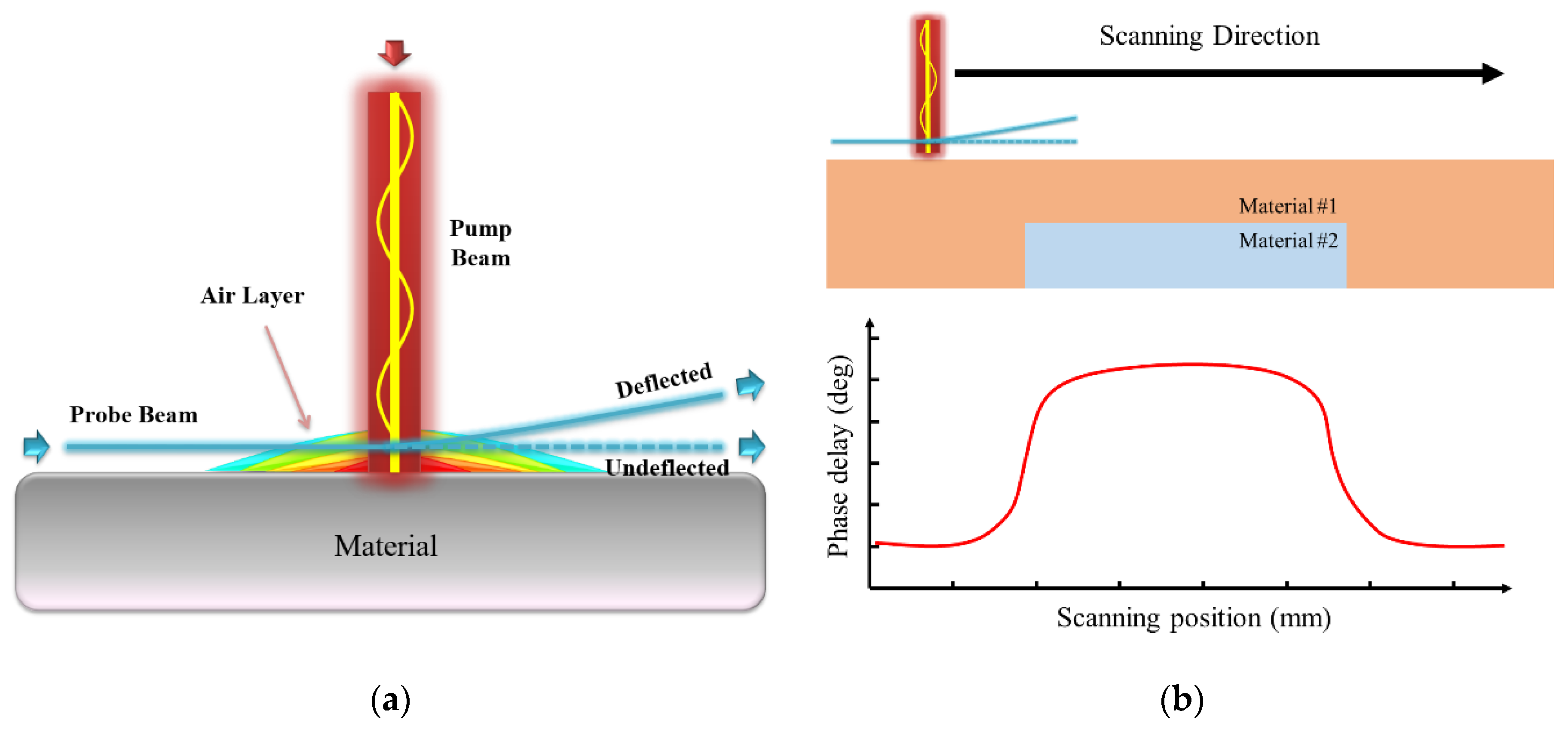
Recently, the photothermal imaging method has been studied as an industrial tomographic tool. It acquires morphological information from the inside of an object by means of the photothermal effect of a temporally modulated heat source [1,2,3,4]. The photothermal effect is a physical phenomenon that occurs when a material absorbs light energy and converts it to thermal energy [5,6]. As shown in Figure 1a, when a material is heated by a temporally modulated pump beam, the temperature of both the air layer on the material surface together and the material itself increases as heat is conducted from the material to the air. In addition, the refractive index of the air layer changes with temperature because of the density change. It is possible to achieve a modulated temperature change through the refraction of the probe beam that passes through the air layer. The physical phenomena that result from the photothermal effect are based on the thermal properties of the target material to be measured. Hence, the phase delay between the period of the refraction of the probe beam and that of the heat source (light energy) must be analyzed in order to acquire information on the thermal properties of the specimen [7,8,9,10,11]. This method can be applied to imaging. As illustrated in Figure 1b, when the surface of a material is scanned by the pump beam and probe beam, the phase delay changes as the thermal properties are changed by the distribution of internal materials.

This photothermal imaging method has been studied for more than ten years by McDonald, Wetsel, and Friedrich [12,13,14], since Murphy and Aamodt published a study on how to acquire morphological information on a subsurface internal structure from the phase delay [4]. The related studies to the photothermal imaging method have been focused on the possibility of detecting subsurface structures using photothermal signals (phase delay). Previous studies have shown that the photothermal imaging method is experimentally feasible. However, there have been attempts to study the quality of images acquired from the photothermal imaging method. Therefore, the limitation of measurement in photothermal imaging has not been investigated or reported.

The applicability of the developed imaging method depends on the image quality for the image of the internal structure acquired from the imaging method. Image quality is represented by spatial resolution, contrast, sharpness, and other metrics, and the scope of imaging method applicability depends on these factors [15,16,17].

Image quality varies with the type of imaging method, specifically owing to the configuration of the components of the relevant equipment, the characteristics of the object to be measured, and the measuring system operator′s skills. Analyzing how such factors affect image quality not only requires comprehensive and complicated tasks, but is also of great importance in evaluating a given imaging method [13,14,15].

The image quality analysis techniques and processes are well established. However, the quality of images acquired from the photothermal imaging method has not been quantitatively analyzed. Moreover, no one has investigated whether the image quality analysis techniques can be applied to photothermal imaging. The present study was carried out to analyze image quality by focusing on the contrast and spatial resolution of an imaging method that utilizes the photothermal effect. In addition, the factors that influence the acquired images from the photothermal imaging method are investigated, expecting to provide experimental measurement conditions for the photothermal imaging method.

2. Image Quality Analysis Theory for Photothermal Imaging

2.1. Contrast

Contrast is a measure of the difference between the magnitude of signals from an internal structure and those from the surrounding or background of the internal structure. In general, the purpose of an imaging method is to examine the inside of an object to be measured and to detect any structural differences from the intended design or any abnormal defects. In order to easily detect such defects, imaging methods with high contrast are preferred [18].

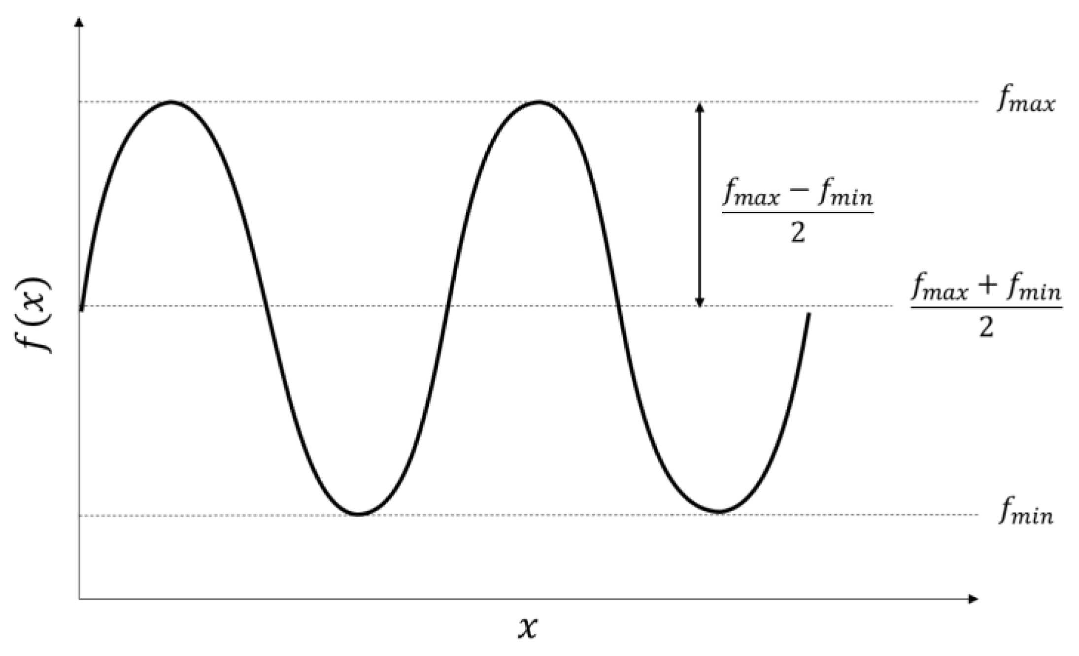
This section focuses on the modulation index that quantifies contrast in reference to periodic signals of constant amplitude, as shown in Figure 2.

The modulation index ($m_{freq}$) of a periodic signal $f\left(x\right)$ whose maximum and minimum amplitudes of signal are $A_{max}$ and $A_{min}$, respectively, can be defined as Equation (1) [18,19], where it is the ratio of the average value of this signal ($\left(A_{max}+A_{min}\right)/2$) to the size of the amplitude ($\left(A_{max}-A_{min}\right)/2$) of the periodic signal $f\left(x\right)$.

$$m_{freq}=\frac{A_{\max }-A_{\min }}{A_{\max }+A_{\min }}.$$

(1)

In the case of an imaging method that utilizes the photothermal effect, as with other imaging methods, the contrast changes depending on the size of the object to be measured (in this study, the size of the internal structure). The size of an object to be measured can be quantified on the basis of the spatial frequency, which can be derived by applying the Fourier transform to a spatial structure in the space. In summary, an imaging method′s contrast can be quantified from the modulation index, and the size of a structure to be measured can be quantified from the spatial frequency [15,17]. The relation between the spatial frequency and modulation index is called the modulation transfer function (MTF). The MTF of an imaging method can be calculated by either of the following methods:

A

For line pairs of varied sizes, the modulation index of a spatial frequency corresponding to each line pair is calculated [20,21].

B

A Fourier transform is applied to the line spread function (LSF) derived from line pairs of the same size [20,21].

The first method (Method A), which uses line pairs of varied sizes, is the most typical way to derive the MTF, but it is disadvantageous in that a large number of specimens is required in order to derive the entire MTF profile. For this reason, comparing the MTF in various conditions drastically increases the number of numerical analyses or experiments.

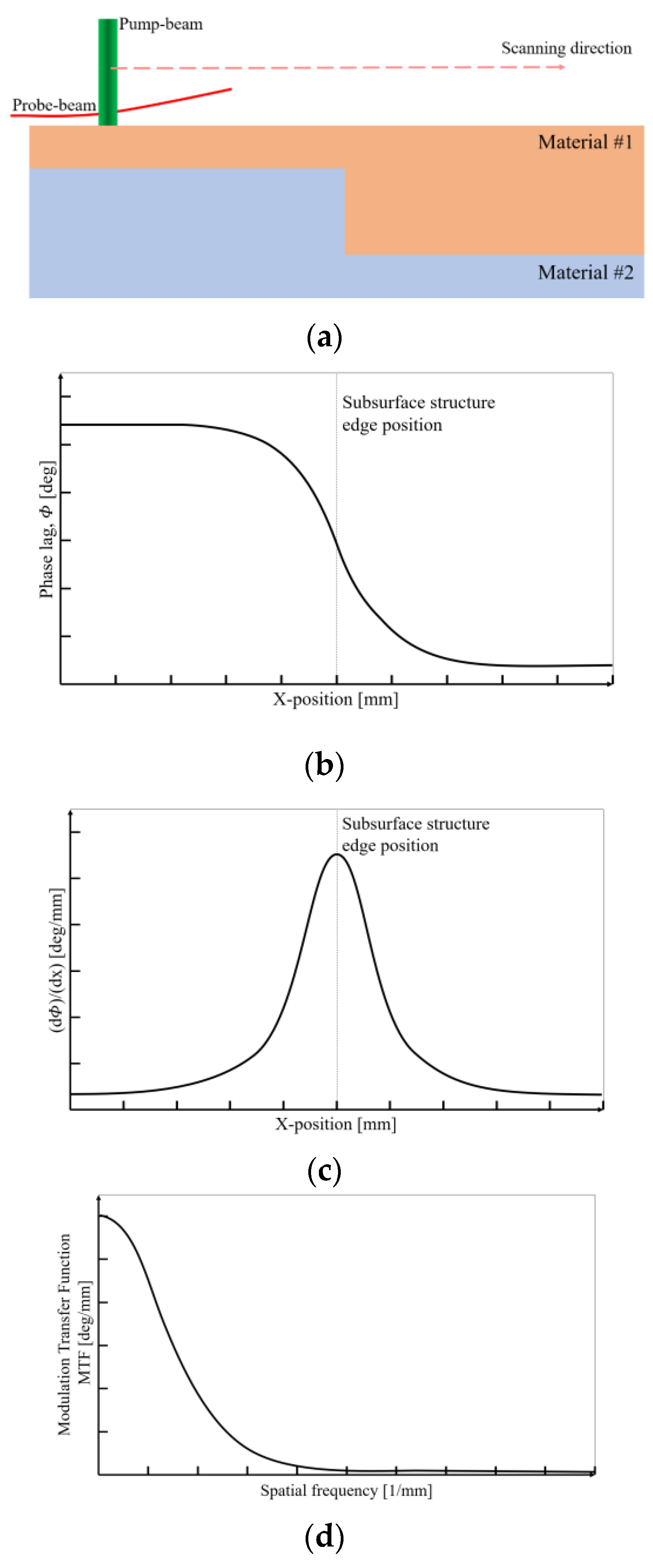
The second method (Method B), which utilizes the LSF, can be implemented in a relatively simple manner [21]. On the assumption that there are infinite specimens with the internal structure shown in Figure 3a in the x- and y-directions, 1-D scanning on the specimen surface using the photothermal imaging method will produce the phase delay change results shown in Figure 3b. The sigmoidal phase difference signal derived near the boundary shown in this figure is called the edge response function (ERF). As the ERF is differentiated, the LSF as in Figure 3c can be obtained.

$$MTF(f_s)=\mathcal{F}\left[LSF(x)\right].$$

(2)

Physically and mathematically, the LSF and MTF are in the relation of a Fourier transform as in Equation (2) [18]. By normalizing the results of applying the Fourier transform to the LSF, the MTF of the imaging system can be derived as shown in Figure 3d.

These two methods of deriving the MTF (Methods A and B) have been found in a number of studies to have the same mathematical and physical meanings [15,20]. The present study derived the MTF by using the relatively simpler Method B and verified contrast changes depending on the spatial frequency.

2.2. Spatial Resolution

The spatial resolution also presents a quantified value of image quality. The spatial resolution can be viewed as the ability of a measuring system to accurately distinguish two different objects at a certain distance from each other [15,17,18].

The determination of spatial resolution begins with the LSF. The LSF can be viewed as a response of the imaging system to line impulses (a linear boundary of the internal structure). Hence, the spatial resolution is determined from the form and size of the LSF [13,15,16]. Many studies have clarified that the spatial resolution can be quantified through the full width half maximum (FWHM) of the LSF of the imaging system [15,22].

3. Numerical and Experimental Analysis

This study numerically analyzed the effect of parameters of the measuring system (namely, the pump beam modulation frequency and pump beam radius) on the contrast and spatial resolution, specifically in relation to imaging a copper-resin double-layered structure that contains slits. This study also experimentally validated the representative result of numerical analysis.

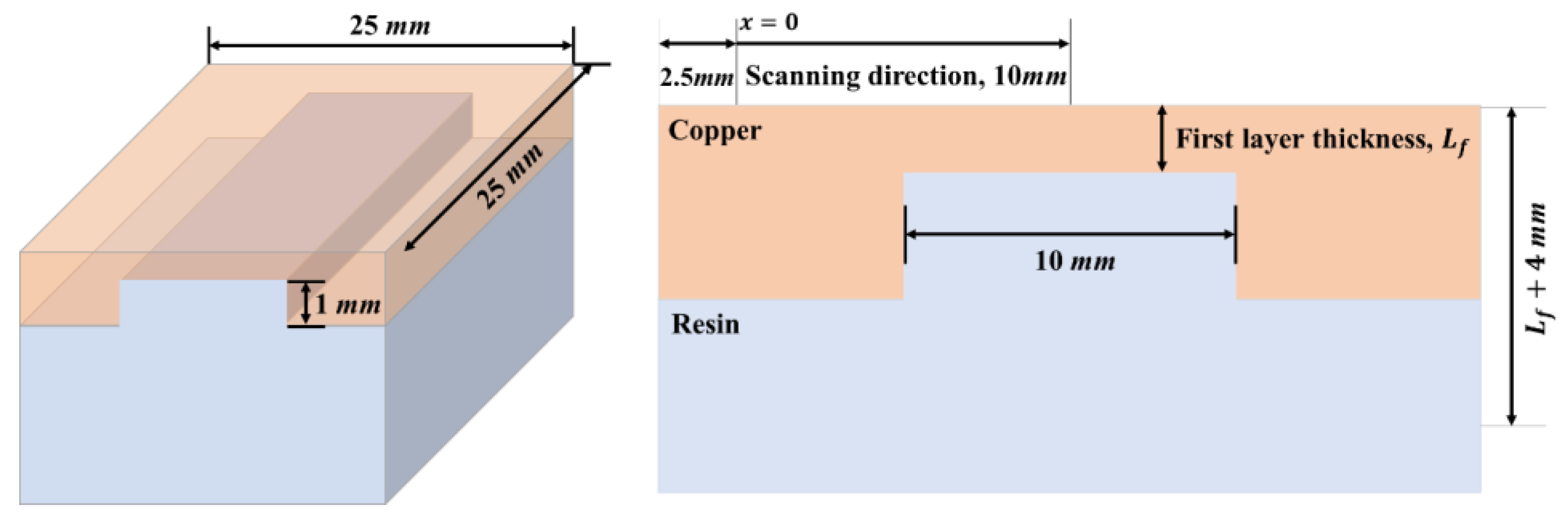
The specimens of the copper-resin double-layered structure that were used in the numerical analysis and experiment are illustrated in Figure 4. The properties of the copper and resin are presented in

Table 1. Thermal properties of the materials [23].

	Copper	Resin	Air
Density ($kg/m^{\mathbf{3}}$)	8930	1050	1.1614
Thermal Conductivity ($W/m·K$)	398	0.51	0.0263
Specific Heat Capacity ($J/kg·K$)	385	500	1007
Thermal Diffusivity ($m^{\mathbf{2}}/s$)	$1.158\times {10}^{-4}$	$9.714\times {10}^{-7}$	$2.249\times {10}^{-5}$

. Additionally, Figure 5 presents the optical arrangement of the specimens and laser applied to the numerical analysis and experiment.

3.1. Setting the Study Parameters

The phase delay signals derived by the photothermal imaging method are significantly affected by the thermal diffusion length ($L_d$), which is expressed as Equation (3) and presented in units of length (m).

$$L_d=\sqrt{\frac{\alpha }{\pi f}}.$$

(3)

Here, $\alpha$ is thermal diffusivity (${\mathrm{m}}^2/\mathrm{s}$) of the material to be measured, and $f$ is modulation frequency (Hz) of the pump beam.

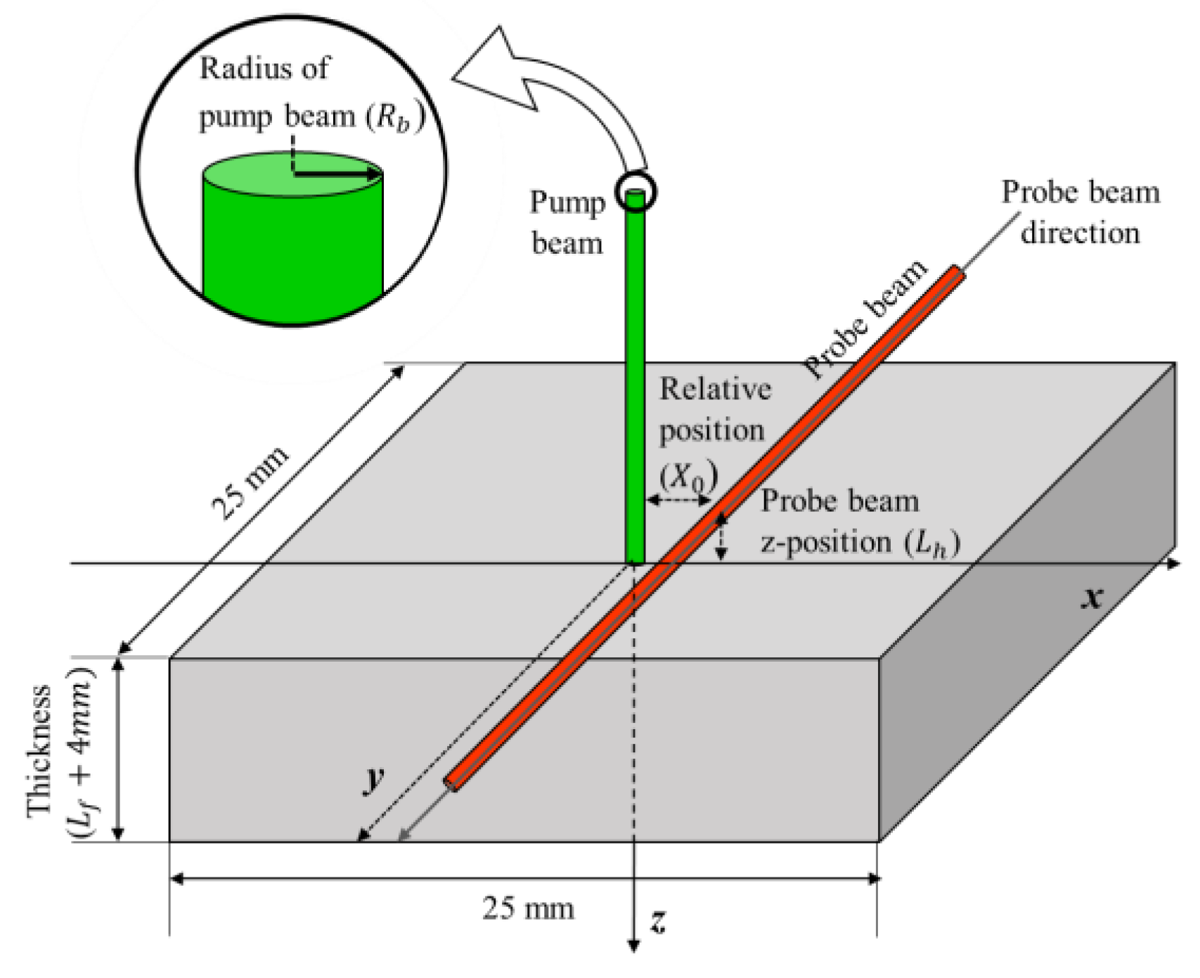
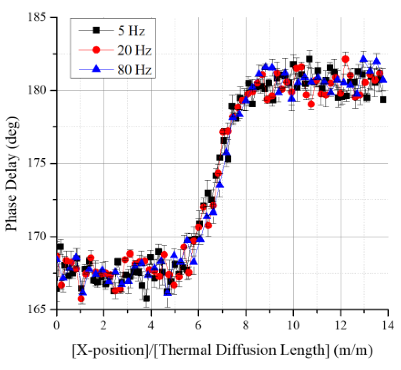
As shown in Figure 5, the length variables of the photothermal imaging method that affect the photothermal effect and phase delay include the pump-beam radius ($R_b$), the thickness of the first layer (here, the copper layer, $L_f$) of the copper-resin double layer, the probe beam’s relative position ($X_0$), and the z-position of the probe beam ($L_h$). Theoretically, if the ratio of each factor to the thermal diffusion length is the same, the same phase delay profile should appear when they are nondimensionalized on the basis of the thermal diffusion length ($L_d$) [1,2,24]. As the experimental results in Figure 6 show, the values of $R_b/L_d$, $L_f/L_d$, $X_0/L_d$, and $L_h/L_d$ are the same in three conditions of different thermal diffusion lengths depending on the pump-beam frequency, as listed in

Table 2. System conditions in Figure 6.

	5 Hz	20 Hz	80 Hz	$\mathbf{Ratio}\mathbf{with}{\mathit{L}}_{\mathit{d}}$
Thermal diffusion length, ${\mathit{L}}_{\mathit{d}}$ (mm)	2.76	1.38	0.69	-
Pump-beam radius, ${\mathit{R}}_{\mathit{b}}$ (mm)	0.40	0.20	0.10	0.145
First-layer thickness, ${\mathit{L}}_{\mathit{f}}$ (mm)	2.00	1.00	0.50	0.725
Relative position, ${\mathit{X}}_{\mathbf{0}}$ (mm)	1.20	0.60	0.30	0.435
z-position of probe beam, ${\mathit{L}}_{\mathit{h}}$ (mm)	0.60	0.30	0.15	0.218

. Thus, they formed the same scanning profile.

Among these factors, the relative position and z-position of the probe-beam ($L_f$) are determined when a photothermal phenomenon is detected or phase delay data are acquired. These do not directly affect the phenomena of the photothermal effect. Hence, the present study derives image quality change related to two parameters: the first (copper) layer thickness ($L_f$) of the copper-resin double-layer and the pump-beam radius ($R_b$).

3.2. Numerical Analysis

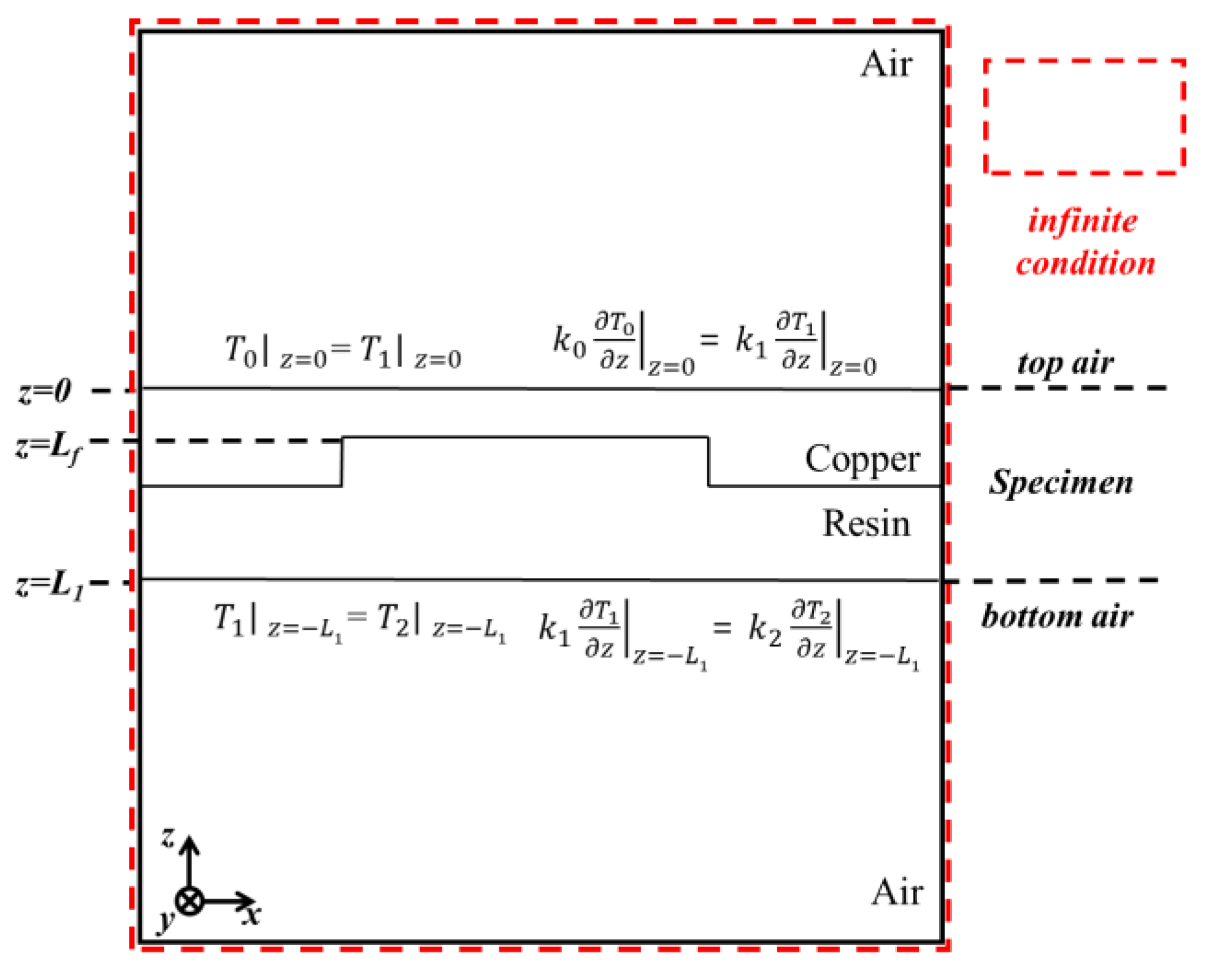
In order to analyze the image quality of the photothermal imaging method, numerical analysis was conducted on specimens with the simple subsurface structure shown in Figure 4. The numerical analysis model had the boundary conditions presented in Figure 7, and it was conducted on the basis of the model established by Kim et al. [3]. Here, the infinite condition means that the physical properties of the adjacent material are infinite [25]. The size and shape of the numerical model specimen are the same as those in Figure 4, and the thickness of the top and bottom air layers is set to 15 mm. Equation (4) is the governing equation for the three areas that consist of three layers: the top air layer, the specimens, and the bottom air layer:

$${\nabla }^2{T}_i+\frac{1}{k_i}{Q}_i=\frac{1}{{\alpha }_i}\frac{\partial T_i}{\partial t}\hspace{1em}(i=\mathit{top}\mathit{air}[0],\mathit{sample}\left[1\right],\mathit{bottom}\mathit{air}\left[2\right])$$

(4)

where the subscript $i$ indicates each domain to be interpreted (0: top air layer, 1: sample, 2: bottom air layer), $T_i$ is the temperature of the layer, $k_i$ is the thermal conductivity of the layer, $t$ is the time, and $Q_i$ indicates the modulated heat source. Equation (5) is the heat source equation for each layer. Here, the light absorption coefficient ($\lambda ,{\mathrm{cm}}^{-1}$) of copper is 623,100 ${\mathrm{cm}}^{-1}$, $a\left({\mathrm{m}}^2\right)$ is the area of the pump beam, and $x_c$ and $y_c$ are the center coordinates of the pump beam, respectively, which are changed to implement laser scanning. $y_c$ is fixed at 0 mm, and $x_c$ is changed from 0 to 10 mm (0.1 mm intervals), as shown in Figure 4.

$$\begin{array}{c}{Q}_1(x,y,z,t)=-\frac{P_0}{4\pi a^2}{e}^{-\lambda z}{e}^{-\left({\left(x-x_c\right)}^2+{\left(y-y_c\right)}^2\right)/a^2}{e}^{iwt}\\ Q_0(x,y,z,t)=0\\ Q_2(x,y,z,t)=0\end{array}$$

(5)

The specific parameters used in the numerical analysis are presented in

Table 3. Study parameters.

Pump beam frequency, $\mathit{f}$ (Hz)	80	1 step
Thermal diffusion length, ${\mathit{L}}_{\mathit{d}}$ (mm)	0.69	1 step
First layer thickness, ${\mathit{L}}_{\mathit{f}}$ (mm)	0.125–1.00	5 steps (equal intervals)
Pump-beam radius, ${\mathit{R}}_{\mathit{b}}$ (µm)	50–400	4 steps (equal intervals)
Relative position, ${\mathit{X}}_{\mathbf{0}}$ (mm)	0.3	1 step
z-position of probe beam, ${\mathit{L}}_{\mathit{h}}$ (mm)	0.15	1 step

. With the other parameters fixed, the numerical analysis was conducted with five different values of the first (copper) layer thickness ($L_f$) and four different values of the pump-beam radius ($R_b$).

3.3. Experimental Apparatus and Setup

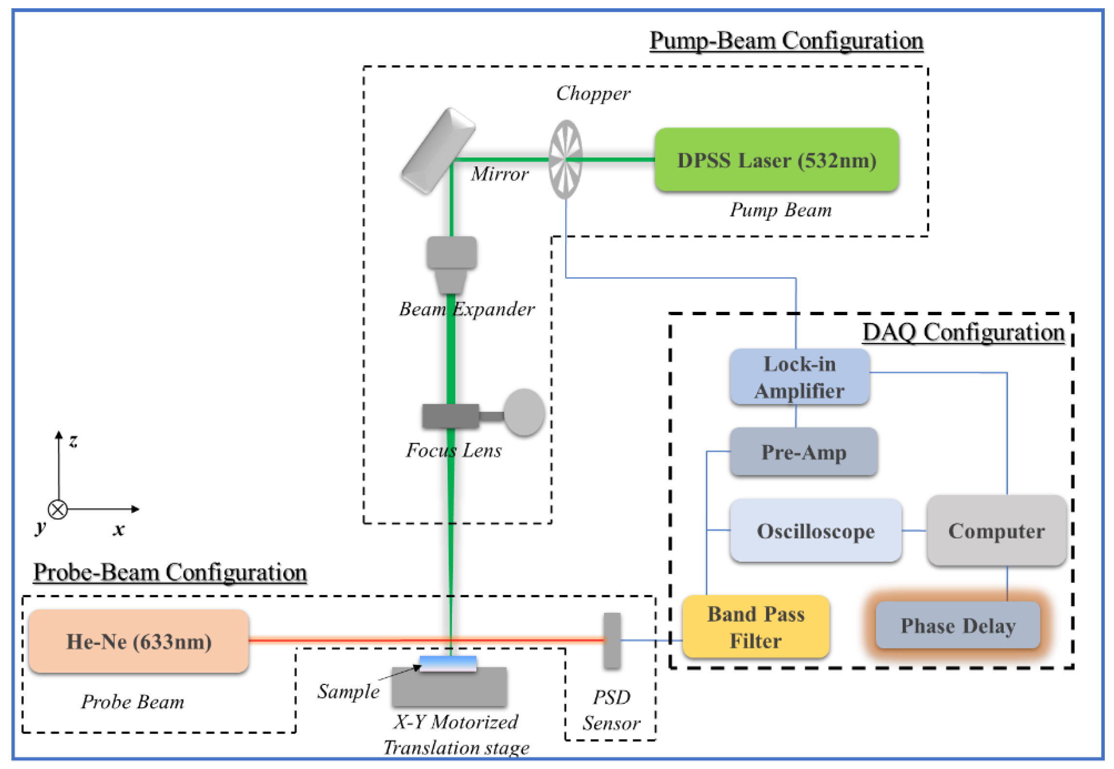
Figure 8 presents the general configuration of the experimental equipment, which consisted mainly of the pump beam, specimen, probe-beam, and data-acquisition configurations. The light source from the pump beam to the probe beam was modulated by a mechanical chopper (SRS 40), passed through a focus lens with a focal length of 1000 mm, and then radiated onto the specimen surface. The intensity of the laser used in this process was 10 W, and a Sprout-G 10-W model with a wavelength of 532 nm, which is a diode-pumped solid-state (DPSS) laser with a Gaussian profile, was used. The radius of the pump beam is determined by the distance from the maximum intensity to $1/{\mathrm{e}}^2$ in the Gaussian distribution [19], and that radius is adjusted by the focus lens. The specimen to be measured was installed at the specimen section. The specimen was mounted on the Newport optic mount and then fixed on an x–y-axis automatic transport system (x-axis: M-IMS300CCHA; y-axis: M-ILS150PP) consisting of two automatic transport units. The probe beam section was located near the specimen section. The probe beam was an He–Ne laser (Newport 1125 P) with a wavelength of 632.8 nm, an intensity of 5 mW, and a diameter of 500 µm. The modulated refraction of the probe-beam that passed through the air layer on the heated specimen was detected by the position sensitive diodes (PSD) sensor (C10443-01). Thereafter, the reference modulation frequency set by the mechanical chopper and the probe-beam response frequency detected by the PSD sensor were collected by the lock-in amplifier (AMETEK 7270 DSP), and the phase difference between the two signals was calculated. Figure 5 presents the arrangement and relative distance between the probe-beam and pump beam.

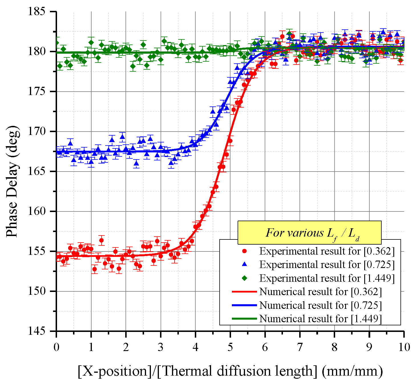
The numerical analysis results were verified by experimentally examining the image quality depending on the $L_f/L_d$ change. Specifically, experiments were conducted on specimens with $L_f$ value of 0.25 mm, 0.50 mm, and 1.00 mm (with $L_f/L_d$ values of 0.362, 0.725, and 1.449, respectively), and the pump-beam radius ($R_b$) was fixed at 100 µm. The other parameters were set as shown in Table 3.

4. Results of Numerical Analysis

As mentioned above, the 1-D scanning results were numerically analyzed while changing the first layer thickness ($L_f$) and the pump-beam radius ($R_b$). In order to clarify common tendencies in a number of results according to each parameter change, changes in image quality were examined mainly for two groups: one group in which $R_b$ was fixed at 100 µm ($R_b/L_d=$ 0.145) and another group in which $L_f$ was fixed at 0.5 mm ($L_f/L_d=0.725$). Additionally, every graph presented in this section was nondimensionalized on the basis of the thermal diffusion length.

4.1. Image Quality Change with $L_f/L_d$

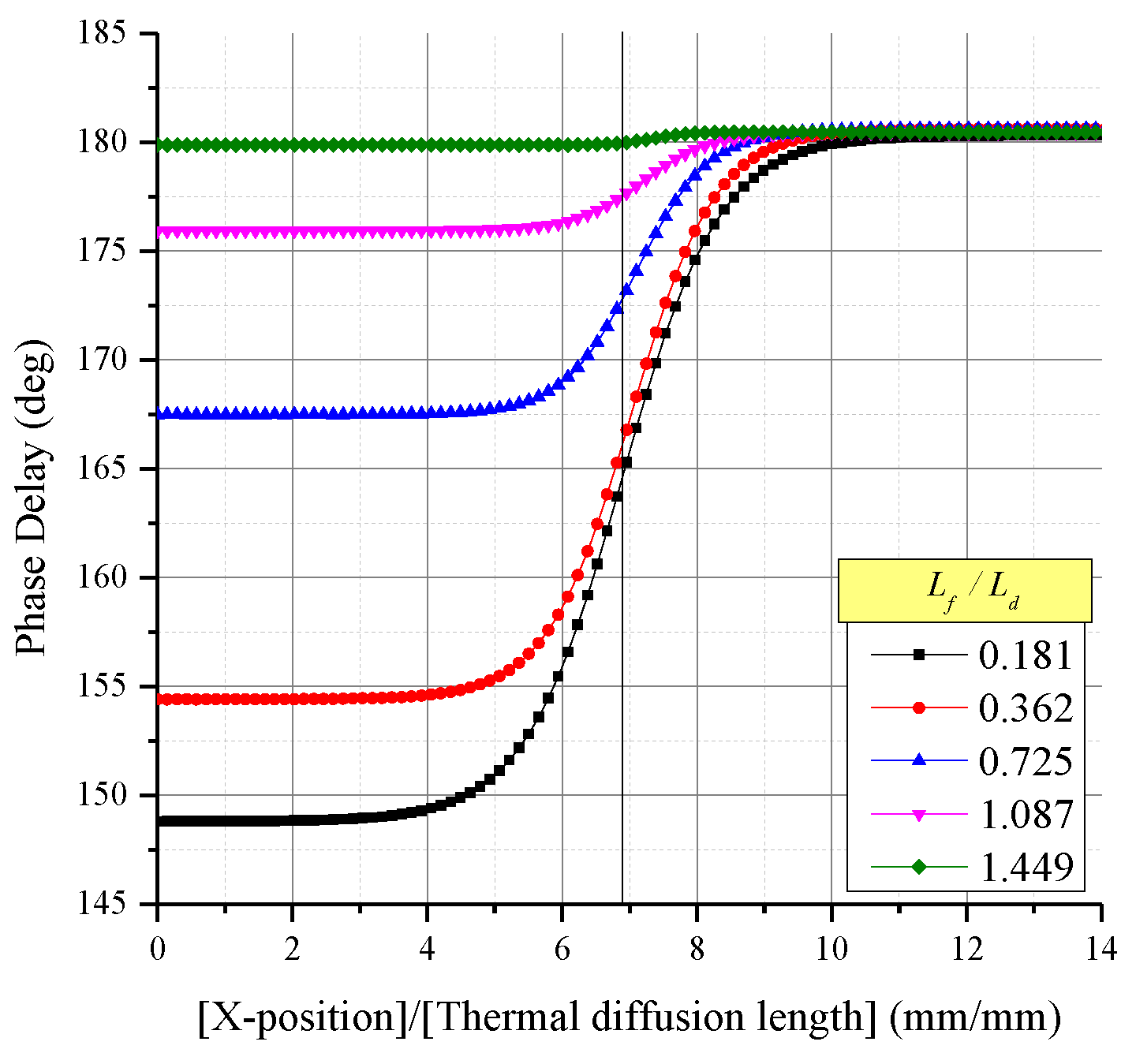
Figure 9 shows the phase delay signals (the ERF on the internal structure) derived by the photothermal imaging method with changed various of $L_f/L_d$. As $L_f/L_d$ decreased (closer to the surface), the response to the internal structural change became more intense. As $L_f/L_d$ increased (i.e., farther from the surface), the response weakened.

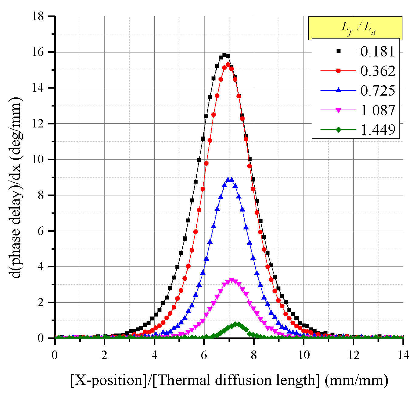
The LSF can be obtained by differentiating the ERF as shown in Figure 10. Thus, the spatial resolution from the LSF can be analyzed. As mentioned previously, the spatial resolution of the imaging system is the FWHM of the LSF. Figure 9 indicates that, as $L_f/L_d$ increases (located deeper), the FWHM decreases. In other words, the spatial resolution is improved. The spatial resolutions for five different values of $L_f/L_d$ are summarized in

Table 4. Spatial resolution and contrast depending on the change according to $L_f/L_d$ ($R_b$ was fixed to 100 µm, $R_b/L_d=$ 0.145).

	${\mathit{L}}_{\mathit{f}}/{\mathit{L}}_{\mathit{d}}$
	0.181	0.362	0.725	1.087	1.449
Dimensionless resolution (mm/mm)	2.549	2.191	1.881	1.775	0.903
Dimensionless contrast (mm/mm)	0.155	0.180	0.206	0.223	0.433

.

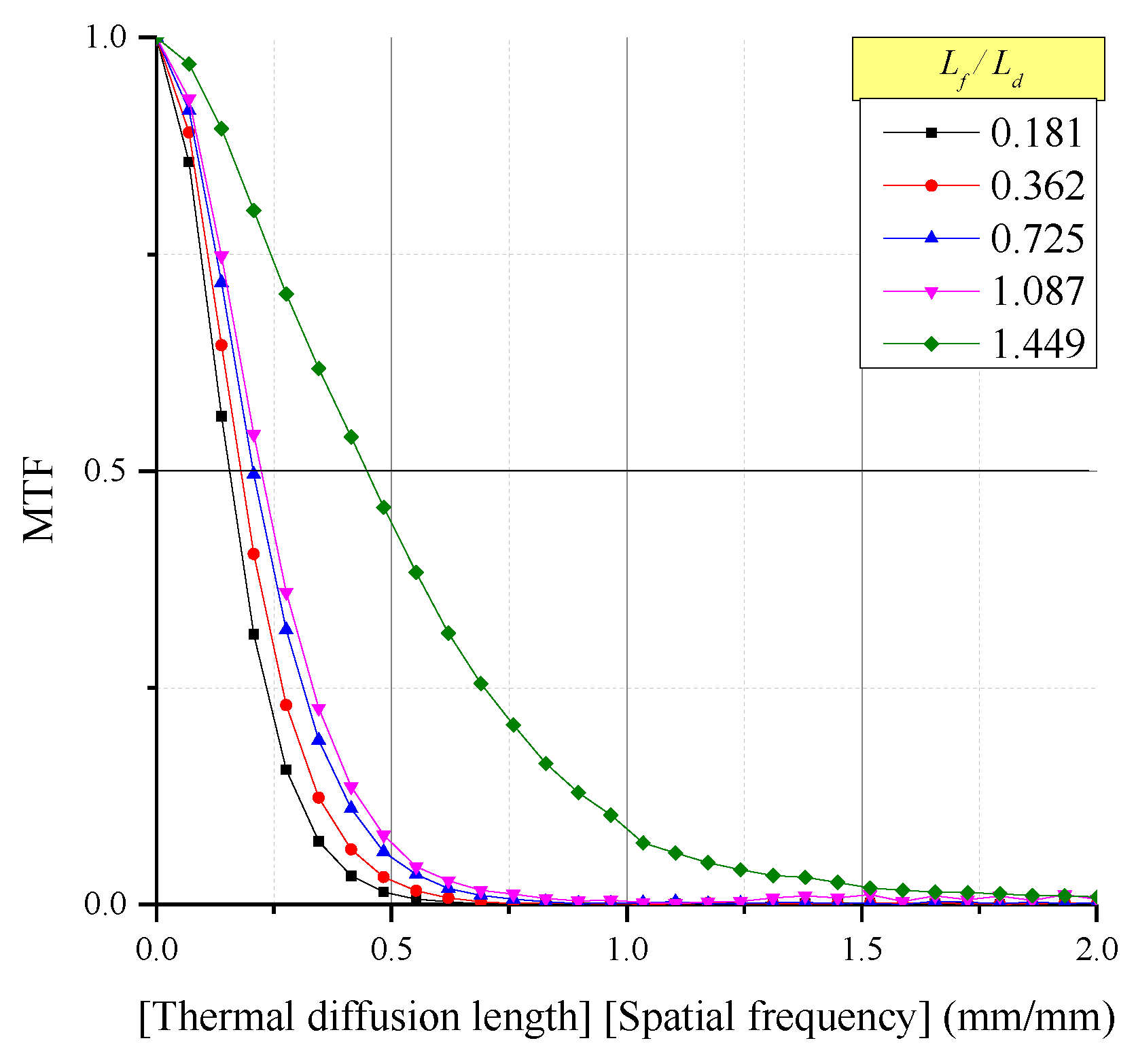
The contrast was verified from the MTF derived by applying the FFT to the LSF. Figure 11 shows the contrast according to the change of $L_f/L_d$. As in the case of spatial resolution, the contrast increased together with $L_f/L_d$. In the case of the MTF, it is difficult to compare the general tendency on the basis of a single value. Instead, Table 4 presents the dimensionless spatial frequency (the thermal diffusion length multiplied by the spatial frequency) at which the MTF became 0.5 and the contrast decreased by half.

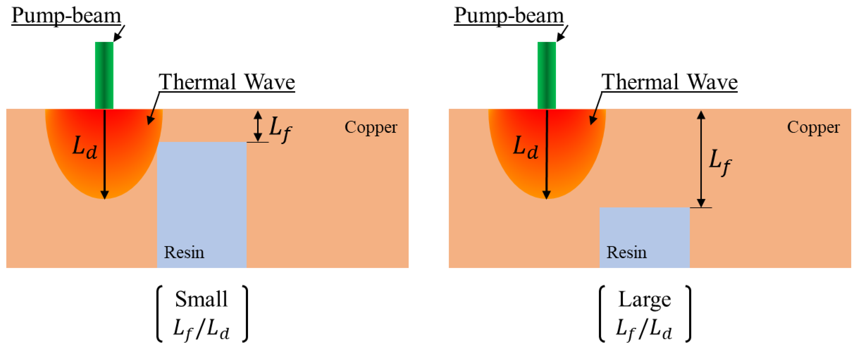
The changes in the spatial resolution and contrast according to $L_f/L_d$ revealed that, as $L_f/L_d$ increased, the spatial resolution and contrast increased accordingly. A small $L_f/L_d$ means that the subsurface structure (resin structure) within the range of the thermal wave has a large influence, and a large $L_f/L_d$ means that this influence is small. Figure 12 depicts the physical phenomena depending on $L_f/L_d$. As shown in Figure 12, when a thermal wave of the same size exists in the same position, the subsurface structure can be detected when $L_f/L_d$ is small but cannot be detected when $L_f/L_d$ is large. For this reason, as $L_f/L_d$ increases, the FWHM of the LSF decreases and the resolution increases. However, the photothermal imaging signal should come from the phase delay, which reflects the distribution of the thermal properties within the range of the thermal wave. Therefore, if $L_f/L_d$ is large, the influence of the subsurface structure on phase delay becomes small, so the intensity of the ERF decreases.

Therefore, as $L_f/L_d$ reached a certain level, the intensity of the ERF decreased significantly. Hence, it is estimated that experimental detection would be impossible, according to the signal noise analysis by the photothermal imaging method suggested by Kim et al. [2].

4.2. Image Quality Change with $R_b/L_d$

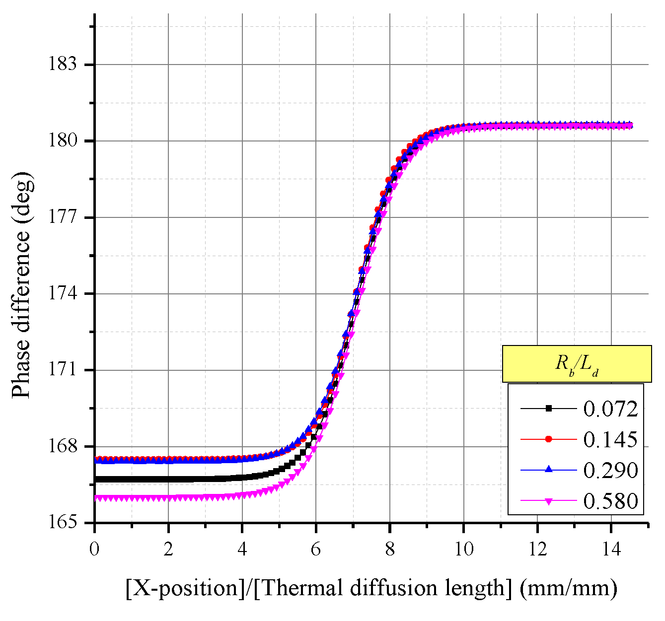
Figure 13 shows the ERF according to changes in $R_b/L_d$. Unlike the case of $L_f/L_d$, there was a minor change in the ERF intensity as $R_b/L_d$ increased in the case of $R_b/L_d$.

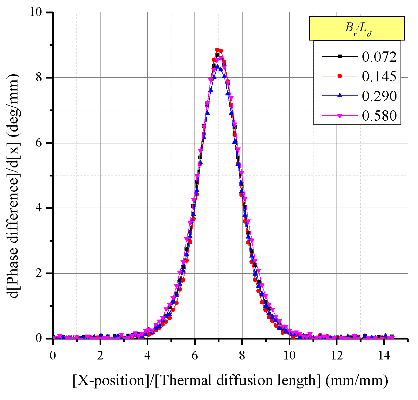
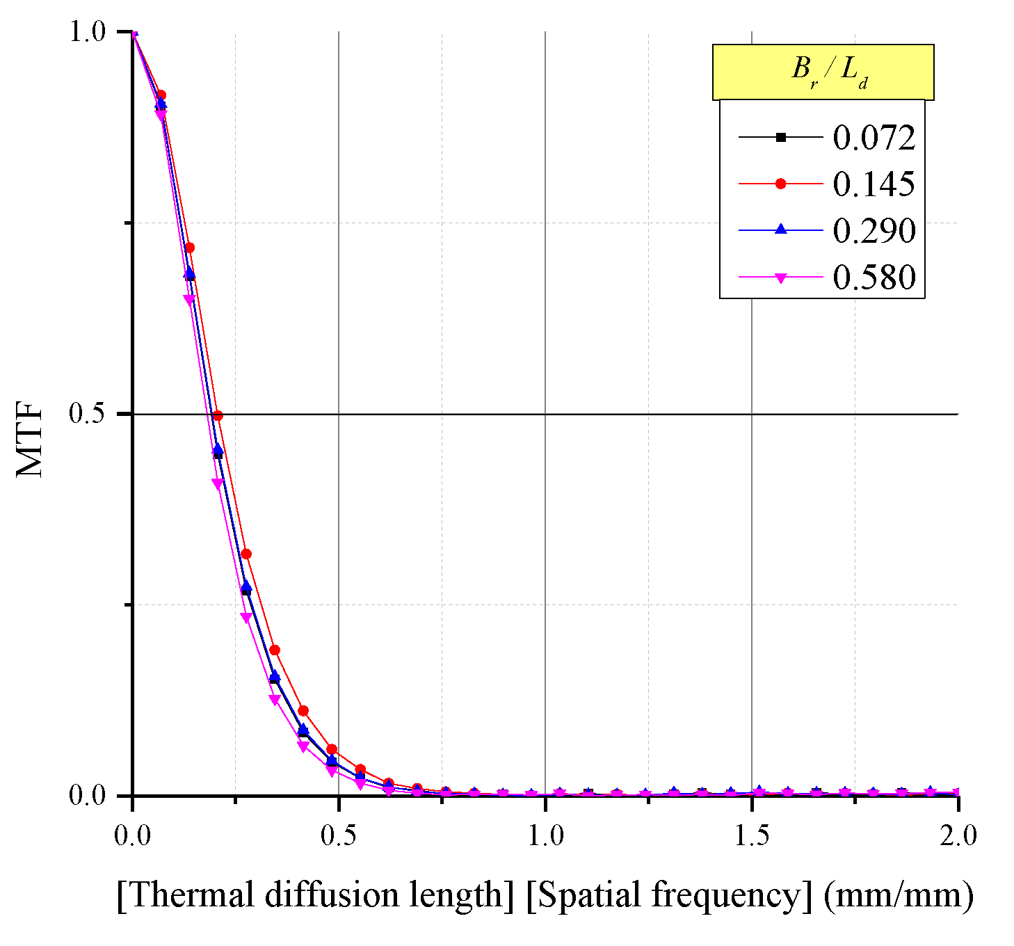
Because the ERF change was insignificant, the LSF also showed no major change. As a result, the spatial resolution change derived from the LSF, as shown in Figure 14, showed a difference of only 10% from the average. The MTF indicating the contrast in Figure 15 also showed the same tendency. In addition, the positions where the contrast decreased by half showed a difference of less than 10% from the average. The reason for this is that the diameter of the thermal wave in the radial direction cannot have influences on the detection of subsurface structure.

Numerical analysis was conducted for each of the 20 cases in which both $L_f/L_d$ and $R_b/L_d$ changed, as well as the cases in which each parameter was fixed, and the results are presented in

Table 5. Image quality depending on changes in ${\mathit{L}}_{\mathit{f}}$ and ${\mathit{R}}_{\mathit{b}}$.

	${\mathit{R}}_{\mathit{b}}/{\mathit{L}}_{\mathit{d}}$	${\mathit{L}}_{\mathit{f}}/{\mathit{L}}_{\mathit{d}}$
		0.181	0.362	0.725	1.087	1.449
Dimensionless resolution (mm/mm)	0.072	2.557	2.196	2.050	1.804	0.756
	0.145	2.549	2.191	1.881	1.775	0.903
	0.290	2.555	2.188	2.027	1.812	0.840
	0.580	2.561	2.193	2.167	1.768	1.091
Dimensionless contrast (mm/mm)	0.072	0.153	0.177	0.191	0.217	0.568
	0.145	0.155	0.180	0.206	0.223	0.433
	0.290	0.153	0.177	0.193	0.212	0.459
	0.580	0.153	0.177	0.181	0.223	0.373

. Likewise, the image quality change according to changes in $R_b/L_d$ was insignificant. In contrast, for the image quality change according to changes in $L_f/L_d$, the spatial resolution increased as $L_f/L_d$ increased.

This tendency suggests that the pump-beam radius has an insignificant effect on image quality and that an increase in $L_f/L_d$ within an experimentally measurable range is essential to achieve good image quality.

5. Results of Experimental Analysis

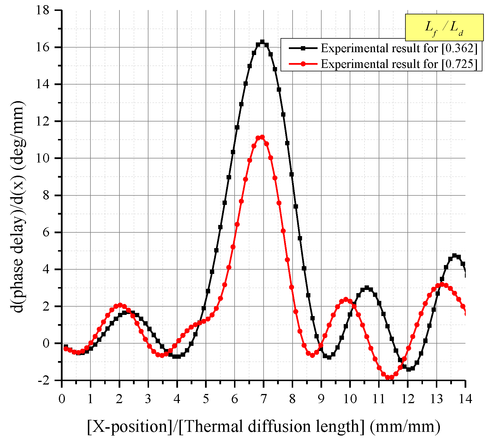
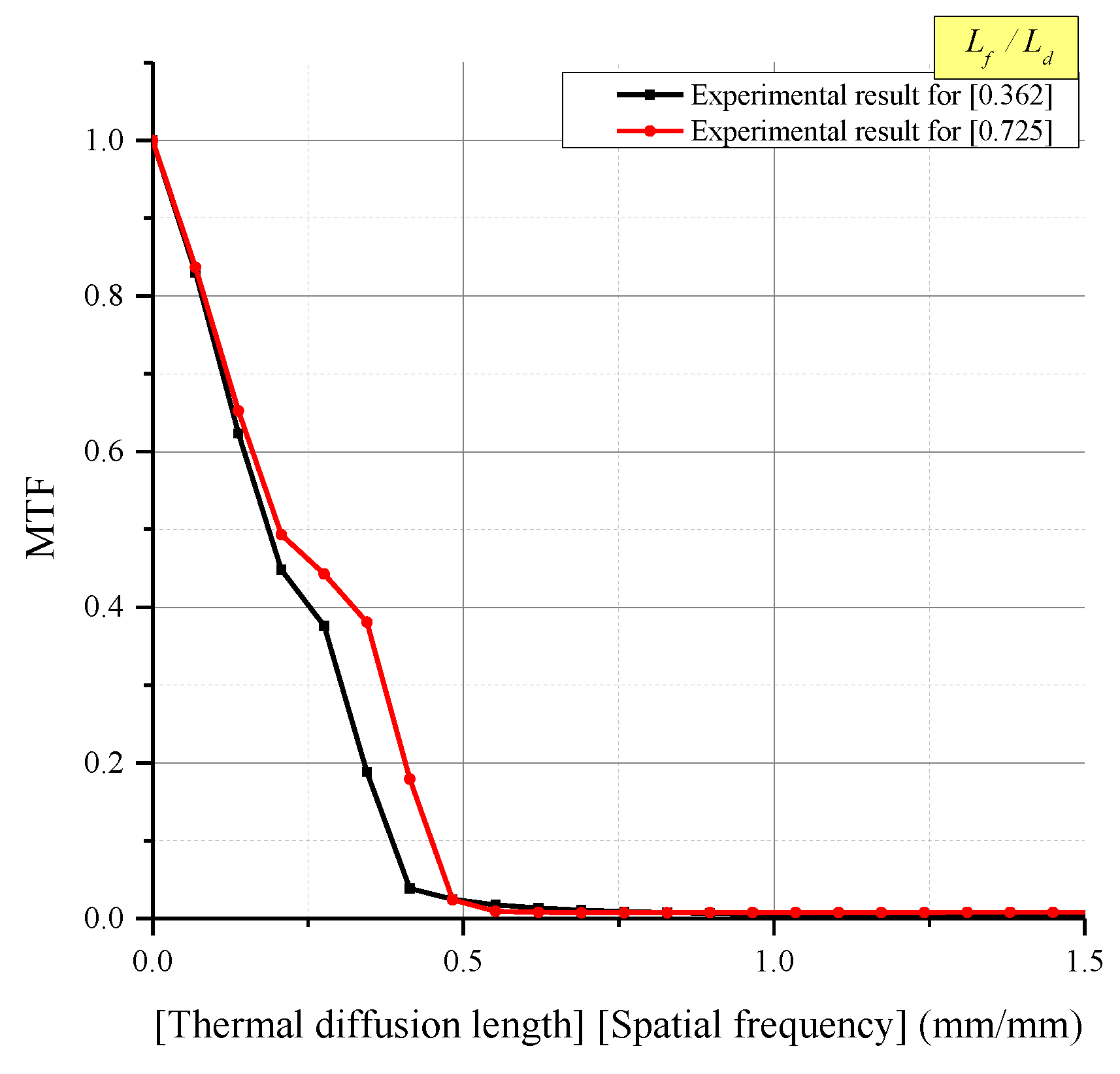
Figure 16 shows the ERF measured in the experiments in comparison with the numerical analysis results. It was found that the numerical analysis results corresponded well with the experimental results, with a determination coefficient ($R^2$) of 0.974. Noise was removed from the experimental results by means of the low-pass fast Fourier transform (FFT) filter proposed by Kim et al. The LSF (Figure 17) was then derived, and the MTF (Figure 18) was derived from the FFT in order to analyze the image quality. However, when the ratio of $L_f/L_d$ was 1.449, it was difficult to obtain a smoothed ERF through the removal of noise. This is because the intensity of the noise is larger than intensity of the ERF, as shown in Figure 18. Therefore, it was impossible to carry out the analysis of image quality. For this reason,

Table 6. Image quality in the experimental results according to changes in $L_f/L_d$.

	${\mathit{R}}_{\mathit{b}}/{\mathit{L}}_{\mathit{d}}$	${\mathit{L}}_{\mathit{f}}/{\mathit{L}}_{\mathit{d}}$
		0.362	0.725	1.449
Dimensionless resolution (mm/mm)	0.150	2.344	1.743	none
		7%	8%	-
Dimensionless contrast (mm/mm)	0.150	0.187	0.204	none
		4%	1%	-

does not indicate the spatial resolution and contrast for the $L_f/L_d$ of 1.449. When the numerical analysis results were compared with the experimental results for the final spatial resolution and contrast according to each $L_f/L_d$ value, the difference was within 8% in all cases.

6. Conclusions

In this study, the image quality changed according to different measuring conditions, which included the depth of a subsurface structure from the surface of the object (first layer thickness, $L_f$) and the pump-beam radius ($R_b$). As image quality metrics, the spatial resolution and contrast were derived from the FWHM of the LSF and the MTF.

• It was verified that the phase delay profile (edge response function, ERF) of the subsurface structure derived by the photothermal imaging method could be nondimensionalized in relation to the thermal diffusion length. Therefore, various studies on $L_f/L_d$ and $R_b/L_d$ can be conducted to quantitatively analyze the spatial resolution and contrast of photothermal imaging regardless of the absolute size and thermal properties of the material to be measured.
• Analyzing the spatial resolution and contrast under different measuring conditions revealed that, as the ratio of $L_f/L_d$ increases, the spatial resolution and contrast increase as well. On the other hand, the ratio of $R_b/L_d$ has an insignificant effect on the spatial resolution and contrast.
• The range of thermal waves that vary with $L_d$ has a significant effect on the spatial resolution and contrast of photothermal imaging. $L_d$ can be adjusted by the thermal diffusivity of the material to be measured and the modulation frequency of the pump beam as shown in Equation (3). Therefore, to increase the spatial resolution and contrast, it is advantageous for the photothermal imaging method to select $L_d$, which is relatively short compared to $L_f$.
• As the $L_f/L_d$ increases, however, the influence of the subsurface structure within the range of the thermal wave decreases. This means that the phase delay change may not reflect the subsurface structure. Therefore, the photothermal imaging method in large $L_f/L_d$ is not effective for the measurement.
• In conclusion, the image quality analysis of this paper is expected to provide a validation method for the results of photothermal imaging and effective measurement conditions for the photothermal imaging method.

These results suggest that the experimentally measurable spatial resolution and contrast can be improved if the signal-to-noise ratio of the photothermal imaging system can be increased. The noise of a photothermal signal can be controlled by the surface roughness of the specimen to be measured and the pump-beam intensity of the photothermal imaging system [2]. Therefore, in future research, image quality can be analyzed according to the magnitude of noise in the photothermal imaging method.

References

- Kim, M.; Yoo, J.; Kim, D.-K.; Kim, H. Development on the reconstruction of photothermal imaging method for subsurface structure. J. Vis. 2018, 22, 329–339. [Google Scholar] [CrossRef]
- Kim, M.; Kim, G.; Yoo, J.; Kim, D.-K.; Kim, H. Experimental study on the influence of surface roughness for photothermal imaging with various measurement conditions. Thermochim. Acta 2018, 661, 7–17. [Google Scholar] [CrossRef]
- Kim, M.; Yoo, J.; Kim, D.-K.; Kim, H. Numerical study on visualization method for material distribution using photothermal effect. J. Mech. Sci. Technol. 2015, 29, 4499–4507. [Google Scholar] [CrossRef]
- Murphy, J.C.; Aamodt, L.C. Optically detected photothermal imaging. Appl. Phys. Lett. 1981, 38, 196–198. [Google Scholar] [CrossRef]
- Murphy, J.C.; Spicer, J.W.M.; Aamodt, L.C.; Royce, B.S.H. Photoacoustic and photothermal phenomena II. In Proceedings of the 6th International Topical Meeting, Baltimore, MD, USA, 31 July–3 August 1989. [Google Scholar]
- Sell, J. Photothermal Investigations of Solids and Fluids; Elsevier: Amsterdam, The Netherlands, 2012. [Google Scholar]
- Jackson, W.B.; Amer, N.M.; Boccara, A.C.; Fournier, D. Photothermal deflection spectroscopy and detection. Appl. Opt. 1981, 20, 1333–1344. [Google Scholar] [CrossRef]
- Bertolotti, M.; Liakhou, G.; Li Voti, R.; Peng Wang, R.; Sibilia, C.; Yakovlev, V.P. Mirror temperature of a semiconductor diode laser studied with a photothermal deflection method. J. Appl. Phys. 1993, 74, 7054–7060. [Google Scholar] [CrossRef]
- Jeon, P.; Lee, E.; Lee, K.; Yoo, J. A theoretical study for the thermal diffusivity measurement using photothermal deflection scheme. Energy Eng. J. 2001, 10, 63–70. [Google Scholar]
- Salazar, A.; Sánchez-Lavega, A.; Fernandez, J. Thermal diffusivity measurements in solids by the ‘‘mirage’’technique: Experimental results. J. Appl. Phys. 1991, 69, 1216–1223. [Google Scholar] [CrossRef]
- Salazar, A.; Sánchez-Lavega, A.; Fernández, J. Thermal diffusivity measurements on solids using collinear mirage detection. J. Appl. Phys. 1993, 74, 1539–1547. [Google Scholar] [CrossRef]
- McDonald, F.A.; Wetsel, G.C., Jr.; Stotts, S.A. Scanned Photothermal Imaging of Subsurface Structure. In Acoustical Imaging; Springer: Berlin/Heidelberg, Germany, 1982; pp. 147–155. [Google Scholar]
- Friedrich, K.; Haupt, K.; Seidel, U.; Walther, H.G. Definition, resolution, and contrast in photothermal imaging. J. Appl. Phys. 1992, 72, 3759–3764. [Google Scholar] [CrossRef]
- McDonald, F.A.; Wetsel, G.C., Jr.; Jamieson, G.E. Spatial Resolution of Subsurface Structure in Photothermal Imaging. In Acoustical Imaging; Springer: Berlin/Heidelberg, Germany, 1985; pp. 377–385. [Google Scholar]
- Prince, J.L.; Links, J.M. Medical Imaging Signals and Systems; Pearson Prentice Hall: Upper Saddle River, NJ, USA, 2006. [Google Scholar]
- Martz, H.E.; Logan, C.M.; Schneberk, D.J.; Shull, P.J. X-ray Imaging: Fundamentals, Industrial Techniques and Applications; CRC Press: Boca Raton, FL, USA, 2016. [Google Scholar]
- Antoniou, A. Digital Signal Processing; McGraw-Hill: New York, NY, USA, 2016. [Google Scholar]
- Staude, A.; Goebbels, J. Determining the spatial resolution in computed tomography–comparison of MTF and line-pair structures. In Proceedings of the International Symposium on Digital Industrial Radiology and Computed Tomography, Ghent, Belgium, 22–25 June 2011; pp. 20–22. [Google Scholar]
- Hecht, E. Optics, 5th ed.; Pearson: London, UK, 2016. [Google Scholar]
- Park, S.K.; Schowengerdt, R.A.; Kaczynski, M.A. Modulation-transfer-function analysis for sampled image systems. Appl. Opt. 1984, 23, 2572. [Google Scholar] [CrossRef] [PubMed]
- 15708-1:2002. Non-Destructive Testing—Radiation Methods—Computed Tomography—Part 1: Principles; The International Organization for Standardization: Geneva, Switzerland, 2002. [Google Scholar]
- Dhawan, A.P. Medical Image Analysis; John Wiley & Sons: Hoboken, NJ, USA, 2011; Volume 31. [Google Scholar]
- Ross, R.B. Metallic Materials Specification Handbook; Springer Science & Business Media: Berlin/Heidelberg, Germany, 2013. [Google Scholar]
- Marín, E. Characteristic dimensions for heat transfer. Lat.-Am. J. Phys. Educ. 2010, 4, 56–60. [Google Scholar]
- Bergman, T.L.; Incropera, F.P.; DeWitt, D.P.; Lavine, A.S. Fundamentals of Heat and Mass Transfer; John Wiley & Sons: Hoboken, NJ, USA, 2011. [Google Scholar]
Figure 1.
Schematic diagram of photothermal imaging: (a) detection of photothermal signals; (b) detection of internal material through scanning.
Figure 2.
Example of periodic signals with a constant amplitude.
Figure 3.
Process of deriving the modulation transfer function (MTF) from the scanning results: (a) Signals of specimens with a subsurface structure, (b) edge response function (ERF) derived through measurements, (c) line spread function (LSF) derived through differentiation, and (d) modulation transfer function derived through the fast Fourier transform (FFT).
Figure 4.
Diagram of specimens used in the numerical analysis and experiment.
Figure 5.
Optical arrangement of the specimens and laser.
Figure 6.
Nondimensionalization of the scanning results using different modulation frequencies.
Figure 7.
Boundary conditions of the numerical analysis model.
Figure 8.
Configuration of the experimental apparatus.
Figure 9.
Boundary response functional performance with changes in .
Figure 10.
Performance of line-spread function (LSF) with changes in .
Figure 11.
Performance of the MTF according to changes in .
Figure 12.
Physical phenomena depending on .
Figure 13.
ERF according to changes in .
Figure 14.
LSF according to changes in .
Figure 15.
MTF according to changes in .
Figure 16.
ERF comparison between the experimental and numerical analysis results.
Figure 17.
LSF of the experimental results.
Figure 18.
MTF of the experimental results.