Smart Obstacle Avoidance Using a Danger Index for a Dynamic Environment

Abstract

The artificial potential field approach provides a simple and effective motion planner for robot navigation. However, the traditional artificial potential field approach in practice can have a local minimum problem, i.e., the attractive force from the target position is in the balance with the repulsive force from the obstacle, such that the robot cannot escape from this situation and reach the target. Moreover, the moving object detection and avoidance is still a challenging problem with the current artificial potential field method. In this paper, we present an improved version of the artificial potential field method, which uses a dynamic window approach to solve the local minimum problem and define a danger index in the speed field for moving object avoidance. The new danger index considers not only the relative distance between the robot and the obstacle, but also the relative velocity according to the motion of the moving objects. In this way, the robot can find an optimized path to avoid local minimum and moving obstacles, which is proved by our experimental results.

1. Introduction

Moving in free space while avoiding collisions within the dynamic environment is known as obstacle avoidance or path planning, which is the backbone of mobile robots. Many well-known path planning algorithms have been proposed in robotics research literature. The reward-based planning algorithms [1,2,3] propose to give the robot a positive reward when it reaches the target, and give the robot a negative reward when it collides with the obstacle. The path is then obtained by maximizing the cumulative future reward. However, due to the discretization of the state and control space, their trajectories are mostly not smooth [4]. The sampling-base planning algorithms, such as the Rapidly exploring Random Tree (RRT) [5] and the Probabilistic Road Maps (PRM) [6], generally connect a series of randomly sampled points from a barrier-free space, and attempt to establish a path from the initial position to the target position. Although their time cost is less, the random sampling introduces the randomness of the planned path. Therefore, we cannot predict the result of the path planner, which is not optimal in general. The grid-based planning algorithms, such as the A* [7] and the Dijkstra’s [8] algorithm, which have been used in the robotic operating systems (ROS), can find the optimal trajectory, but their time cost and memory usage grow exponentially with the dimension of the state space [4]. The novel artificial potential field (APF) developed by Khatib [9,10,11] is a simple and effective path planning method. The theory behind APF is simple and straightforward: it has an attractive potential field for attracting the robot to the target point, and a repulsive potential field for pushing the robot away from obstacles. The APF approach can be used for global and local path planning.

However, there are some inherent problems in traditional artificial potential field approaches: (1) oscillations in the presence of obstacles due to the large move step of the robot; (2) goal nonreachable with obstacles nearby (GNRON); (3) trapped in a local minimum region; and (4) moving obstacles avoidance. Solving these problems has become an interesting topic in the field of APF based path planning [12,13]. Park et al. [14] deal with the local minimum region by filling it with the virtual obstacle. Zhu et al. [15] introduce simulated annealing to look for the global minimum and escape the local minimum region. Doria et al. [16] use the Deterministic Annealing (DA) approach to avoid local minima in APF by adding a temperature parameter into the cost function of the APF approach. The value of the temperature parameter starts to increase until the robot goes away from the local minimum region. Lee et al. [17] propose to use two modes to control the APF, i.e., one mode is to go directly to the target using traditional APF and the other mode uses a new point APF algorithm to avoid collisions with the static obstacle. Mode 1 can be switched to mode 2 when the robot is trapped in a local minimum region or blocked in front of the obstacle. A new direction is synthesized using the robot motion information and direction between the robot and the goal point, which can guide the robot to escape the local minimum region. Weerakoon et al. [18] propose an improved repulsive force for overcoming a local minima problem, which generates a new repulsive force to the primary force when the robot detects an obstacle within its sensory range. The new repulsive force component turns the robot smoothly away from the obstacles. Kim et al. [19] modify the APF approach with the collision cone approach, which adds an artificial force to the existing attractive and repulsive forces when the relative velocity vector between the robot and obstacle is included in a collision cone. The improved resultant force can guide the robot to reach the goal. These algorithms may help the robot to escape the local minimum region in a simple statistic environment, but require to detect whether the robot is trapped in the local minimum region.

For the dynamic environment, the moving objects can affect the performance of the APF. Ge et al. [20] define a virtual force which is the negative gradient of the potential with respect to both relative position and velocity between the robot and the target or obstacles. The motion of the mobile robot is then determined by the total virtual force through the Newtons Law or steering control depending on the driving type of the robot. Cao et al. [21] propose a simultaneous target tracking and moving obstacle avoidance method using a threat coefficient based force function by taking into account the relative velocities of the target with respect to the robot and the relative velocities of the robot with respect to the obstacles. Montiel et al. [22] introduce a parallel evolutionary artificial potential field for the dynamic environment, which makes possible controllability in complex real-world sceneries with dynamic obstacles if a reachable configuration set exists. These methods make decisions according to the relative position and velocity direction between robot and obstacle, but the magnitude of the obstacle speed is not fully considered.

In this paper, we propose a dynamic APF approach (DAPF). The contributions of our work are the following: first, to predict and avoid the local minimum region, we combine the APF with the dynamic window approach [23], which employs a cost function to evaluate simulated trajectories, such that the local minimum region can be found in the prior step, and the robot can avoid the obstacle in a short path without any oscillations. Second, we propose an evolutionary potential field function based on an improved minimum danger index (DI) [24,25], which can plan an optimal path using not only the relative distance and velocity direction information, but also the magnitude information of the robot and obstacle speeds. The robot can make a smart decision to avoid moving obstacles, e.g., if the obstacle moves fast, the robot goes behind the obstacle. We demonstrate the proposed ideas using a real mobile robot system in static and dynamic environment, respectively, which shows the improved performance using our idea.

2. The Proposed Method

In this section, we analyze the problems of the traditional APF approaches and further introduce the proposed idea in detail.

2.1. Dynamic Window Based Artificial Potential Field (DAPF)

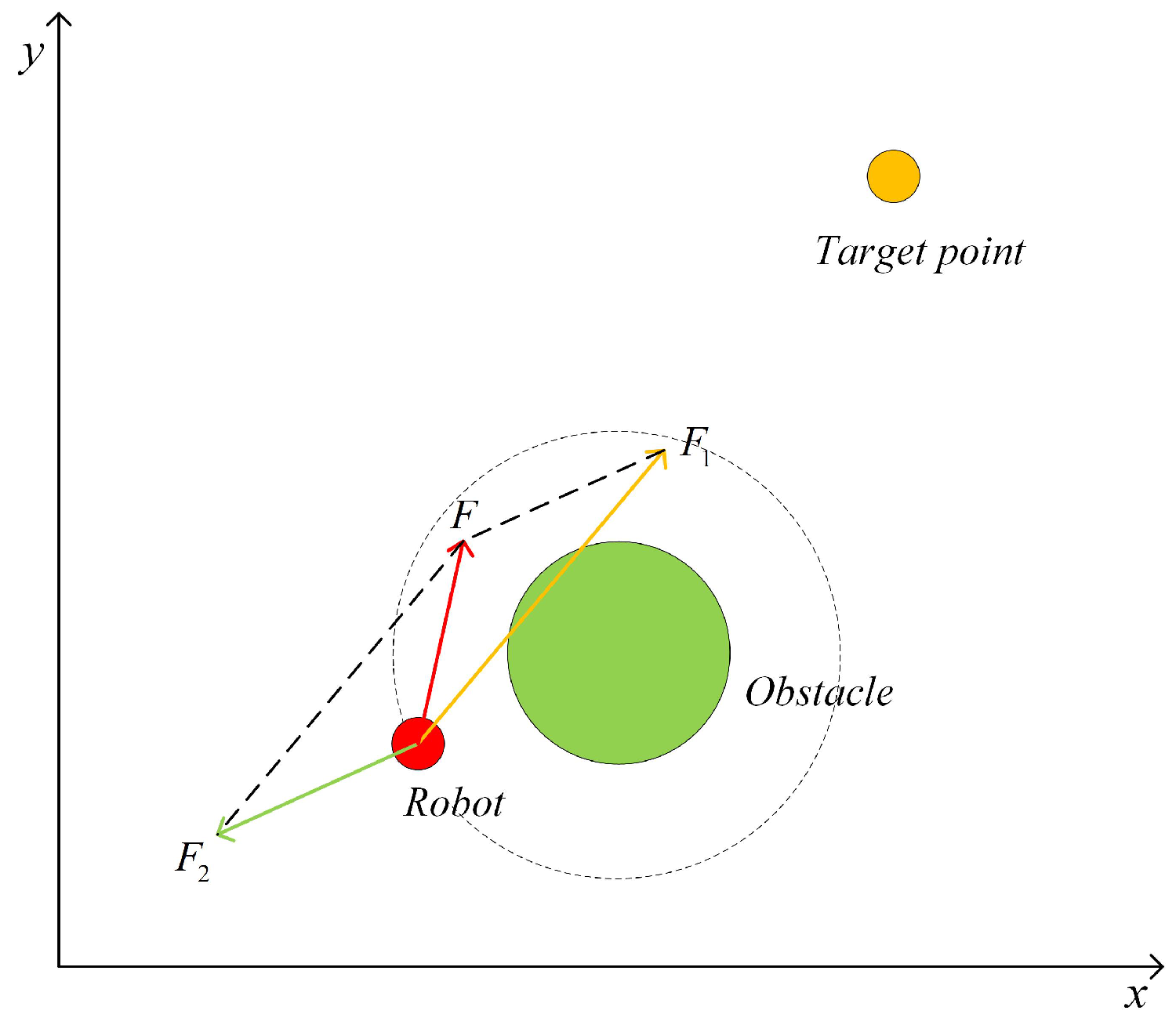
In the artificial potential field, the robot motion is controlled by the attractive force and the repulsive force, i.e., the attractive force is generated by the distance and direction to the target point, whereas the repulsive force is generated by the distance and direction to obstacles. The forces of the robot in the artificial potential field are shown in Figure 1, where $F_2$ is the repulsive force between the obstacle and the robot $F_1$ is the attractive force between the target point and the robot, and F is the resultant force for controlling the robot.

The attractive potential field function is defined as:

$$U_{att}\left(\varphi \right)=\frac{1}{2}{k}_a{(\varphi -{\varphi }_g)}^2,$$

(1)

where $\varphi ={(x,y)}^T$ is the coordinate of the robot, $k_a$ is the coefficient constant of the attractive field, and ${\varphi }_g$ is the coordinate of the target point. The negative gradient of the attractive potential field function is defined as the attractive force function, which is:

$$F_{att}\left(\varphi \right)=-\nabla \left(U_{att}\left(\varphi \right)\right)=k_a({\varphi }_g-\varphi ),$$

(2)

where $F_{att}\left(\varphi \right)$ is a vector directed toward to ${\varphi }_g$, which is a linear correlation with the distance from $\varphi$ to ${\varphi }_g$. Obstacles provide repulsive force and repel the robot. When the robot is far enough from obstacles, obstacles will not affect the motion of the robot. As shown in Equation (3), the repulsion potential field function can be defined as:

$$U_{req}\left(\varphi \right)=\left\{\begin{array}{cc}\frac{1}{2}{k}_r{(\frac{1}{d\left(\varphi \right)}-\frac{1}{d_{max}})}^2,\hfill & d\left(\varphi \right)\le d_{max},\hfill \\ 0,\hfill & d\left(\varphi \right)>d_{max},\hfill \end{array}\right.$$

(3)

where $k_r$ is the coefficient constant of the repulsion field, $d_{max}$ is the maximum impact extent of the single obstacle, and $d\left(\varphi \right)$ is the current distance between the robot and the obstacle. The repulsive force is the negative gradient of the repulsive potential function, which is

$$F_{req}\left(\varphi \right)=-\nabla \left(U_{req}\left(\varphi \right)\right),$$

(4)

$$F_{req}\left(\varphi \right)=\left\{\begin{array}{cc}{k}_r(\frac{1}{d\left(\varphi \right)}-\frac{1}{d_{max}})\frac{1}{d{\left(\varphi \right)}^2}·\frac{\partial d\left(\varphi \right)}{\partial \varphi },\hfill & d\left(\varphi \right)\le d_{max},\hfill \\ 0,\hfill & d\left(\varphi \right)>d_{max}.\hfill \end{array}\right.$$

(5)

The total repulsive potential field is the summation of the repulsive potential fields from all obstacles. The final artificial potential field function is as follows:

$$U\left(\varphi \right)=U_{att}\left(\varphi \right)+\sum U_{req}\left(\varphi \right).$$

(6)

The resultant force on the robot is $F\left(x\right)=F_{att}\left(x\right)+\sum F_{req}\left(x\right)$.

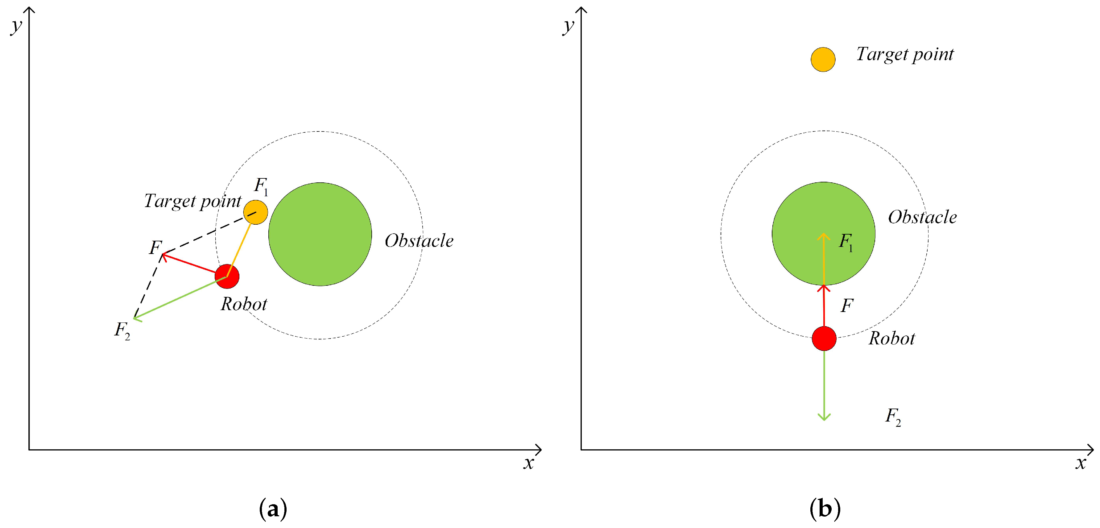
In some situations, the goal can be unreachable and the robot can be trapped in a local minimum region using the traditional APF approach as shown in Figure 2. For instance, the robot can not reach the target point when the target point is very close to the obstacle. In addition, the resultant force on the robot can be reduced gradually until the target point is reached. However, the resultant force of the robot is also likely to be zero or minimized, when the attractive force and repulsive force are almost equal and collinear but in the opposite direction. The robot in this situation is trapped in a local minimum region.

To solve the GNRON problem, the distance between the current position and the target position can be added to the repulsion field function, such that the repulsive force can be relatively reduced when the robot closes to the target point. The improved repulsive potential field function is defined as

$$U_{req}\left(\varphi \right)=\left\{\begin{array}{cc}\frac{1}{2}{k}_r{(\frac{1}{d\left(\varphi \right)}-\frac{1}{d_{max}})}^2{(\varphi -{\varphi }_g)}^n,\hfill & d\left(\varphi \right)\le d_{max},\hfill \\ 0,\hfill & d\left(\varphi \right)>d_{max},\hfill \end{array}\right.$$

(7)

where $k_r$ is the repulsion field coefficient constant and n is an arbitrary real number which is greater than zero. The improved repulsive force function is defined as

$$F_{req}\left(\varphi \right)=\left\{\begin{array}{cc}{F}_{req1}\left(\varphi \right)+F_{req2}\left(\varphi \right),\hfill & d\left(\varphi \right)\le d_{max},\hfill \\ 0,\hfill & d\left(\varphi \right)>d_{max},\hfill \end{array}\right.$$

(8)

where $F_{req1}\left(\varphi \right)$ and $F_{req2}\left(\varphi \right)$ are two components of the $F_{req}\left(\varphi \right)$, which are defined in Equation (9) and (10):

$$F_{req1}\left(\varphi \right)=k_r(\frac{1}{d\left(\varphi \right)}-\frac{1}{d_{max}})\frac{1}{d{\left(\varphi \right)}^2}{(\varphi -{\varphi }_g)}^n·\frac{\partial d\left(\varphi \right)}{\partial \varphi },$$

(9)

$$F_{req2}\left(\varphi \right)=\frac{1}{2}{k}_{r}n{(\frac{1}{d\left(\varphi \right)}-\frac{1}{d_{max}})}^2{(\varphi -{\varphi }_g)}^{n-1}·\frac{\partial (\varphi -{\varphi }_g)}{\partial \varphi }.$$

(10)

The direction of $F_{req1}\left(\varphi \right)$ is from the obstacle to the mobile robot, and $F_{req2}\left(\varphi \right)$ is from the robot to the target point.

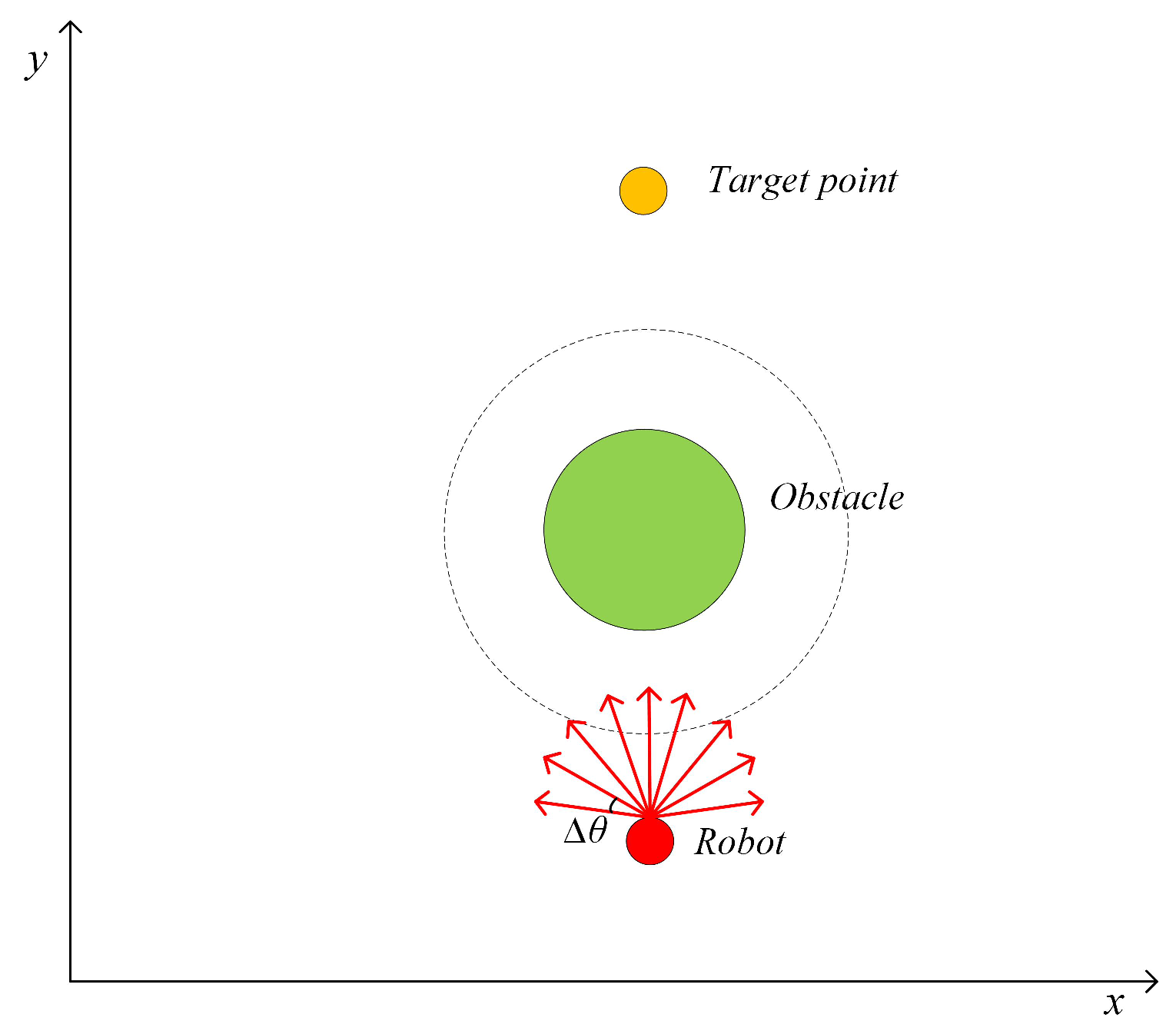
For solving the local minima problem, we propose a dynamic APF approach (DAPF), which employs the dynamic window approach (DWA) to predict the local minimum region and solve the oscillations. The key idea of the DWA is to sample a number of predicted trajectories according to the current position $(x_t,y_t)$, direction ${\theta }_t$ and velocity $v_r$ as shown in Figure 3. The sampled directions ${\theta }_{\omega }$ are the following:

$${\theta }_{\omega }={\theta }_t+(\omega -t)▵\theta ,\omega =(1,\dots ,t,\dots ,n),$$

(11)

where ${\theta }_t$ is the current direction of the robot, $▵\theta$ is the angular step between samples and n is the number of samples. Using these sampled directions, we simulate a number of positions that the robot might go as

$$\left[\begin{array}{cc}{x}_1^{\prime }& y_1^{\prime }\\ \dots & \dots \\ x_t^{\prime }& y_t^{\prime }\\ \dots & \dots \\ x_n^{\prime }& y_n^{\prime }\end{array}\right]=\left[\begin{array}{cc}{x}_t& y_t\\ \dots & \dots \\ x_t& y_t\\ \dots & \dots \\ x_t& y_t\end{array}\right]+\left[\begin{array}{cc}{v}_r▵tcos\left({\theta }_1\right)& v_r▵tsin\left({\theta }_1\right)\\ \dots & \dots \\ v_r▵tcos\left({\theta }_t\right)& v_r▵tsin\left({\theta }_t\right)\\ \dots & \dots \\ v_r▵tcos\left({\theta }_n\right)& v_r▵tsin\left({\theta }_n\right)\end{array}\right],$$

(12)

where $x_1^{\prime },\dots ,x_n^{\prime }$ and $y_1^{\prime },\dots ,y_n^{\prime }$ are coordinates of simulated positions, and $v_r$ is the velocity of the robot. The final choice of the position can be defined as the one whose APF cost function is minimum:

$$\left[\begin{array}{cc}x& y\end{array}\right]=min(APF(\left[\begin{array}{cc}{x}_1^{\prime }& y_1^{\prime }\\ \dots & \dots \\ x_t^{\prime }& y_t^{\prime }\\ \dots & \dots \\ x_n^{\prime }& y_n^{\prime }\end{array}\right])),$$

(13)

where $x,y$ is the coordinate of the position whose resultant force value is minimum.

Based on the improved APF function, the closer the robot is to the target, the smaller the resultant force value is. Before the robot enters the obstacle’s influence range, it applies the DWA approach to simulate positions and calculate the resultant force for every simulated position. If the simulated position is in the obstacle range, the resultant force value is less than 0. If the simulated position is outside of the obstacle range, the resultant force of the simulated position that is closer to the target point is less than the positions that are far from the target point. Finally, the robot can obtain a simulated position that is close to the target point but not in the obstacle area, such that the local minimum region can be avoided using the DAPF approach. If the target point is within the obstacle range, the DWA method will be stopped when the distance of the robot from the target point is less than the distance from the obstacle.

2.2. Danger Index Based Artificial Potential Field (DIAPF) for a Dynamic Environment

To avoid the moving obstacles, the APF must consider not only the position information of the obstacles, but also the motion information of the obstacles, e.g., the direction and magnitude of the velocity. In the paper, we define the motion model of the dynamic obstacle as:

$$\delta (t+1)=\delta \left(t\right)+v_o\left(t\right)\times ▵t,$$

(14)

$$v_o(t+1)=v_o\left(t\right)+a_o^{{}^{\prime }}\left(t\right)\times ▵t,$$

(15)

which can be written in matrix form:

$$p(t+1)=Ap\left(t\right)+a_o,$$

(16)

where $\delta \left(t\right)={(x_o,y_o)}^T$ is the coordinate of the dynamic obstacle, $p(t+1)={(\delta \left(t\right),v_o\left(t\right))}^T$ is the state vector, $A=\left[\begin{array}{cc}1& ▵t\\ 0& 1\end{array}\right]$ is the state transition matrix, and $a_o={(0,a_o^{{}^{\prime }})}^T$ is the acceleration of the dynamic obstacle. In this paper, a uniform motion model is adopted and the $a_o$ is a zero vector.

The APF should not only consider the spatial location of the dynamic obstacle, but also consider the motion state of the dynamic obstacle. Therefore, the velocity repulsive potential field is added to the dynamic window based artificial potential field function (DVAPF) to avoid dynamic obstacles, which is defined as

$$U_v\left(v_{ro}\right)=\left\{\begin{array}{cc}\frac{1}{2}{k}_{ro}{v}_{ro}^2,\hfill & 0\le {\rho }_{cm}\le {\rho }_{cmax}\cap \alpha \in (-\frac{\pi }{2},\frac{\pi }{2}),\hfill \\ 0,\hfill & otherwise,\hfill \end{array}\right.$$

(17)

where $k_{ro}$ is a proportionality constant, $v_{ro}=v_r-v_o$ is the relative velocity between the robot and the dynamic obstacle, $\alpha$ is the angle between the $v_{ro}$ and the vector from the robot to the obstacle, ${\rho }_{cmax}$ is the maximum range of the local map, and ${\rho }_{cm}$ is the current distance between the robot and the dynamic obstacle. The velocity repulsive potential field starts to work when the dynamic obstacle enters the local map whose range is defined by the distance parameter ${\rho }_{cmax}$, which can be chosen according to the sensor range. The velocity repulsive force is the negative gradient of the velocity repulsive potential function:

$$F_v\left(v_{ro}\right)=-\nabla \left(U_v\left(v_{ro}\right)\right),$$

(18)

$$F_v\left(v_{ro}\right)=\left\{\begin{array}{cc}{k}_{ro}{v}_{ro},\hfill & 0\le {\rho }_{cm}\le {\rho }_{cmax}\cap \alpha \in (-\frac{\pi }{2},\frac{\pi }{2})\hfill \\ 0,\hfill & otherwise\hfill \end{array}\right..$$

(19)

The DVAPF approach can handle dynamic obstacle avoidance problem when the velocity difference between the robot and the dynamic obstacle is large. The effectiveness of the velocity repulsive force can be decreased if the relative velocity is small. We here propose an improved method using a novel danger index considering relative distance and velocity between the robot and the dynamic obstacle, which includes three factors:

(1) Distance influence factor:

$$f_{cm}\left({\rho }_{cm}\right)=\left\{\begin{array}{cc}\eta (\frac{1}{{\rho }_{cm}}-\frac{1}{{\rho }_{cmax}}),\hfill & {\rho }_{cm}\le {\rho }_{cmax},\hfill \\ 0,\hfill & {\rho }_{cm}>{\rho }_{cmax},\hfill \end{array}\right.$$

(20)

where $\eta =(\frac{{\rho }_{cmin}{\rho }_{cmax}}{{\rho }_{cmax}-{\rho }_{cmin}})$ is the distance scale factor, and ${\rho }_{cmin}$ is the minimum allowed distance between the robot and the dynamic obstacle.

Distance influence factor is influenced by the distance relationship between the robot and the dynamic obstacle. The closer the distance between the robot and the dynamic obstacle, the larger the distance influence factor.

(2) Speed influence factor:

$$k_o=sgn(\epsilon \times |v_o|-|v_r\left|\right),$$

(21)

where $\epsilon$ is the speed scale factor, $|v_o|$ and $|v_r|$ are the magnitudes of the dynamic obstacle velocity and robot velocity, respectively, and $sgn\left(\right)$ is the sign function.

Speed influence factor is influenced by the speed relationship between the robot and the dynamic obstacle. If the speed of the dynamic obstacle is $\epsilon$ times the speed of the robot, the speed influence factor is an integer and vice versa.

(3) Danger index:

$$DI=\left\{\begin{array}{cc}{k}_{ro}(v_r-f_{cm}{v}_o),\hfill & k_o>0\cap \alpha \in (-\frac{\pi }{2},\frac{\pi }{2})\cap f_{cm}>0,\hfill \\ k_{ro}(v_r+f_{cm}{v}_o),\hfill & k_o\le 0\cap \beta \in (-\frac{\pi }{2},\frac{\pi }{2})\cap f_{cm}>0,\hfill \\ 0,\hfill & otherwise,\hfill \end{array}\right.$$

(22)

where $k_{ro}$ is a proportionality constant, $f_{cm}$ is the distance influence factor, $\alpha$ is the angle between the $(v_r-f_{cm}{v}_o)$ and the vector from the robot to the obstacle. $\beta$ is the angle between the $(v_r+f_{cm}{v}_o)$ and the vector from the obstacle to the robot.

The novel danger index includes distance influence factor and speed influence factor. The robot can make smarter avoidance decisions according to the speed influence factor, i.e., the robot can move in front of the moving obstacle if the speed of the robot is not larger than $\epsilon$ times that of the dynamic obstacle, whereas the robot can move behind the moving obstacle for other situations.

If the distance between the robot and the dynamic obstacle is very close, the distance influence factor will be large, such that the robot will move parallel with the dynamic obstacle, which is to ensure the safety of the path. If the distance between the robot and the dynamic obstacle is far, the distance factor will be small, such that the robot will not over-react to the obstacle motion, which can increase the efficiency of the robot motion. Furthermore, if the moving obstacle is outside of the local map, i.e., ${\rho }_{cm}>{\rho }_{cmax}$, the danger index is 0, so the robot will not react to such a situation.

The danger index combines the distance influence factor and the speed influence factor to optimize the planned path to avoid dynamic obstacles. The danger index based APF (DIAPF) function is defined as

$$U^{{}^{\prime }}\left(\varphi \right)=U\left(\varphi \right)+\frac{1}{2}D{I}^2,$$

(23)

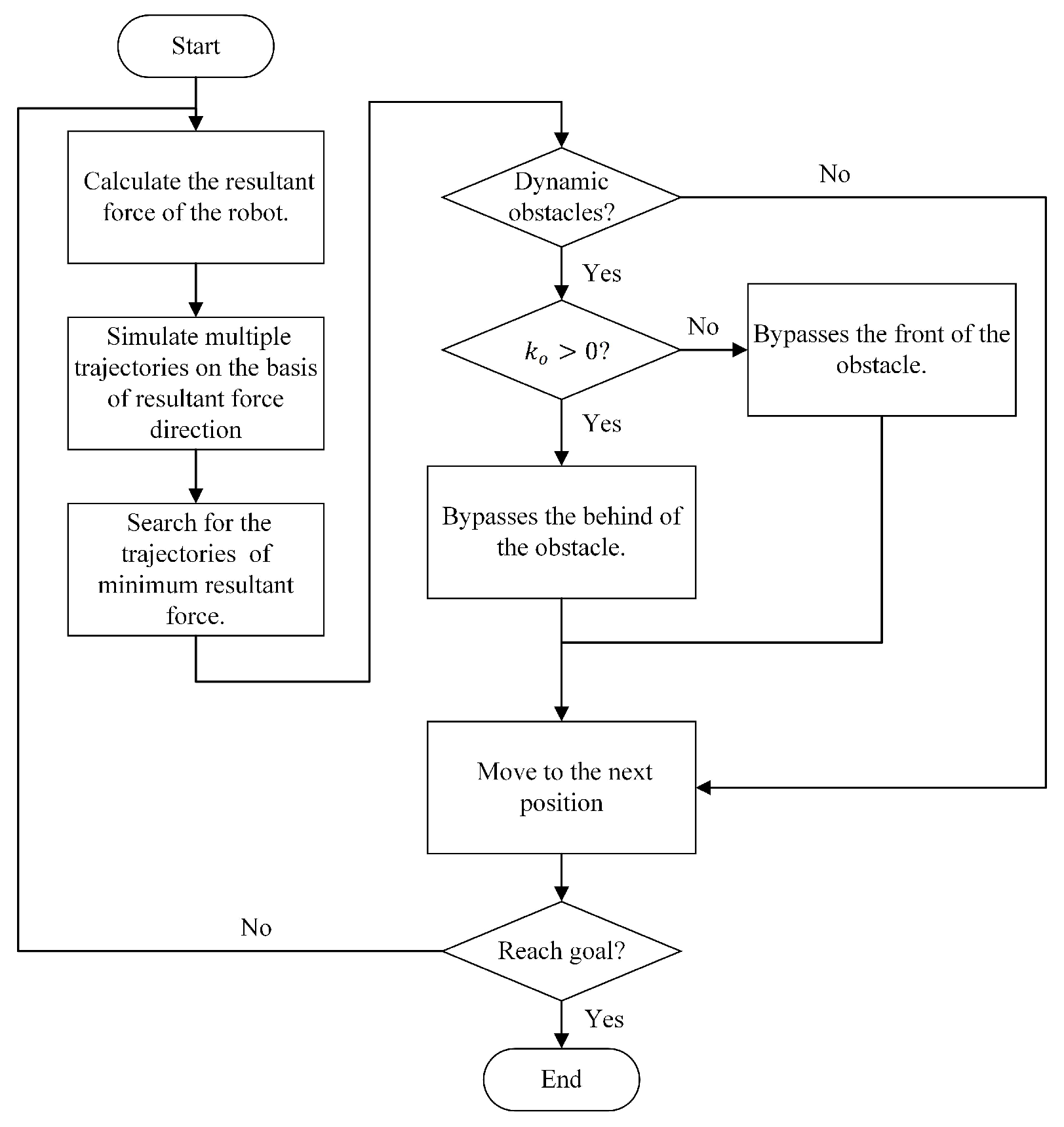
where $U\left(\varphi \right)$ is the value returned from the DAPF function. To summarize, the whole algorithm of our proposed DIAPF approach in the dynamical environment is shown in Figure 4.

3. Experiment and Analysis

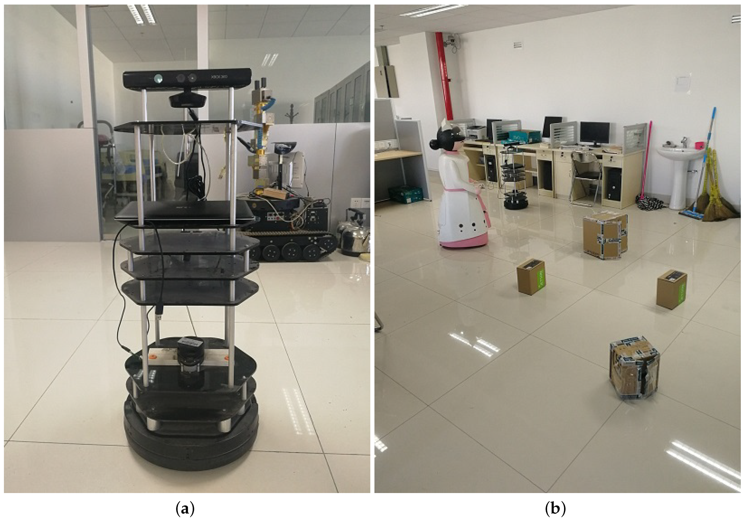
To evaluate the performance of the proposed idea, we use a Turtlebot robot to demonstrate the algorithm in the real environment where we have built a known map. The nurse robot plays as a moving obstacle in the map. To simplify the problem, the map of the environment and the motion status of the obstacle (nurse robot) are known for the Turtlebot. The Turtlebot robot and experimental environment are shown in Figure 5. We first compare the DAPF to the standard APF approach in the static environment to show how the dynamic window approach can improve the performance of the APF, and then compare the DIAPF with the DAPF, the DVAPF and ROS (robot operating system) path planning algorithm to show how the danger index can help the robot avoid the moving obstacle.

3.1. Static Environment

For a static environment, we place several obstacles randomly in the room. The DAPF and the standard APF algorithms are carried out using the experimental parameters defined in

Table 1. The experimental parameters in a static environment.

${\mathit{d}}_{\mathit{max}}$	$▵\mathit{\theta }$	${\mathit{k}}_{\mathit{r}}$	${\mathit{k}}_{\mathit{a}}$	m	n	Target Point
0.2 m	10${}^{\circ }$	1	1	1	2	(2.5, 2.5)

.

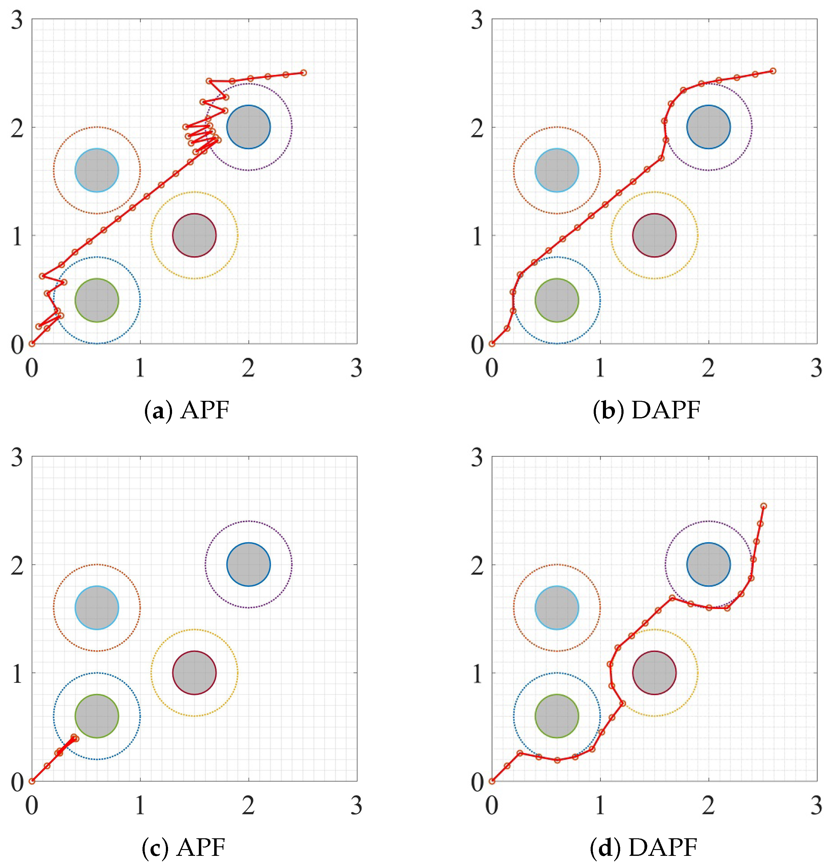
The robot has the oscillation problem and can not avoid the local minimum region using the standard APF algorithm as shown in Figure 6a,c, respectively. In contrast to the APF, the proposed DAPF approach has a smooth planned path along the edge of the influence range of obstacles as shown in Figure 6b,d. For the local minimum problem, the DAPF has no need to detect whether the robot has entered a local minimum region, since the DWA can predict and avoid such a situation in advance.

3.2. Moving Obstacle

For dynamic environment, we compare three methods to avoid the moving obstacle, i.e., DAPF, DVAPF and DIAPF. We show that these methods have different performance for faster and slow moving obstacles. The experimental parameters are shown in

Table 2. The experimental parameters for moving obstacle avoidance

${\mathit{k}}_{\mathit{r}\mathit{o}}$	$\mathit{\epsilon }$	${\mathit{\rho }}_{\mathit{m}\mathit{a}\mathit{x}}$	${\mathit{\rho }}_{\mathit{m}\mathit{i}\mathit{n}}$	${\mathit{v}}_{\mathit{r}}$	${\mathit{v}}_{\mathit{o}}$ (fast)	${\mathit{v}}_{\mathit{o}}$ (slow)
1	2	1.2 m	0.3 m	0.2 m/s	0.3 m/s	0.1 m/s

.

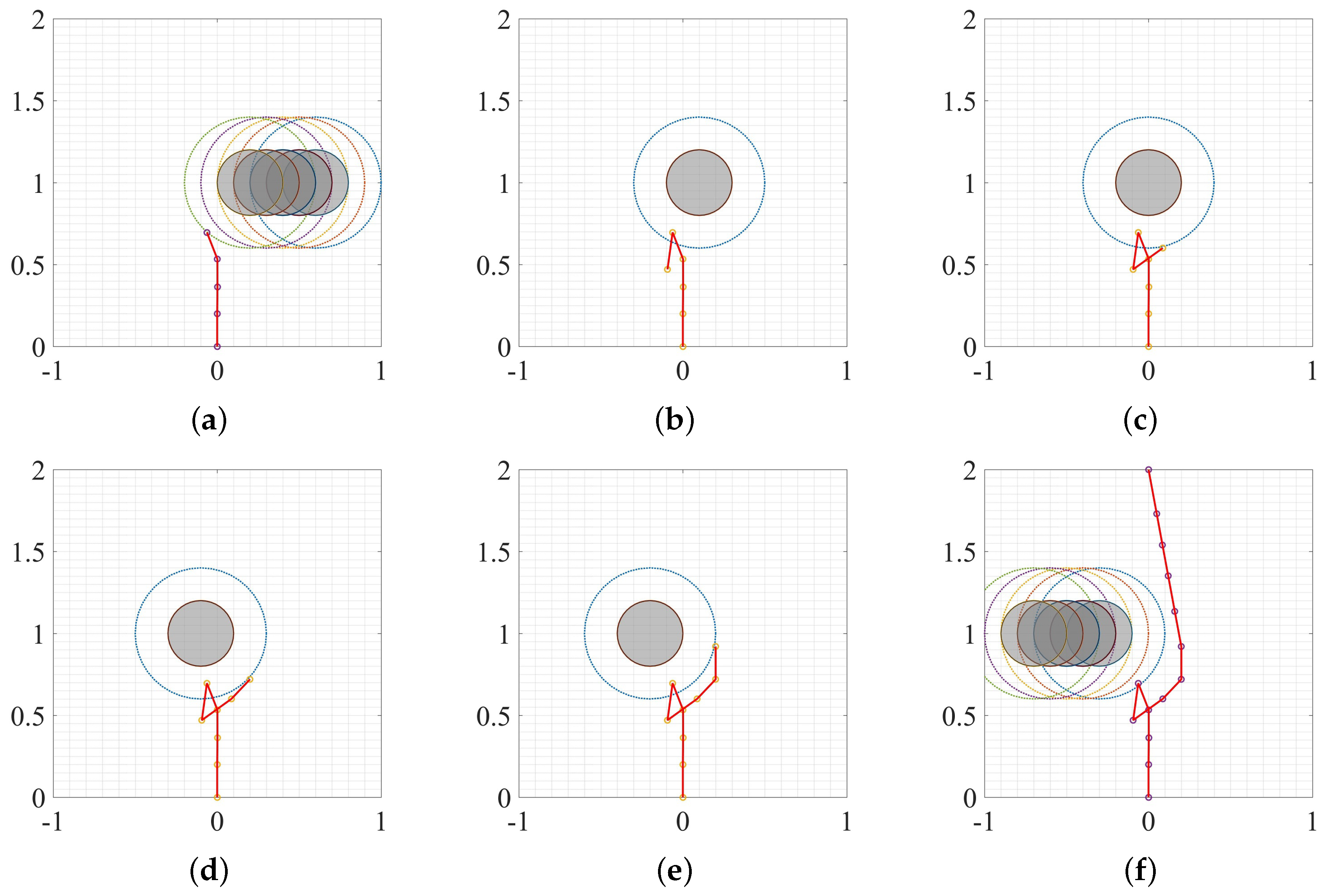
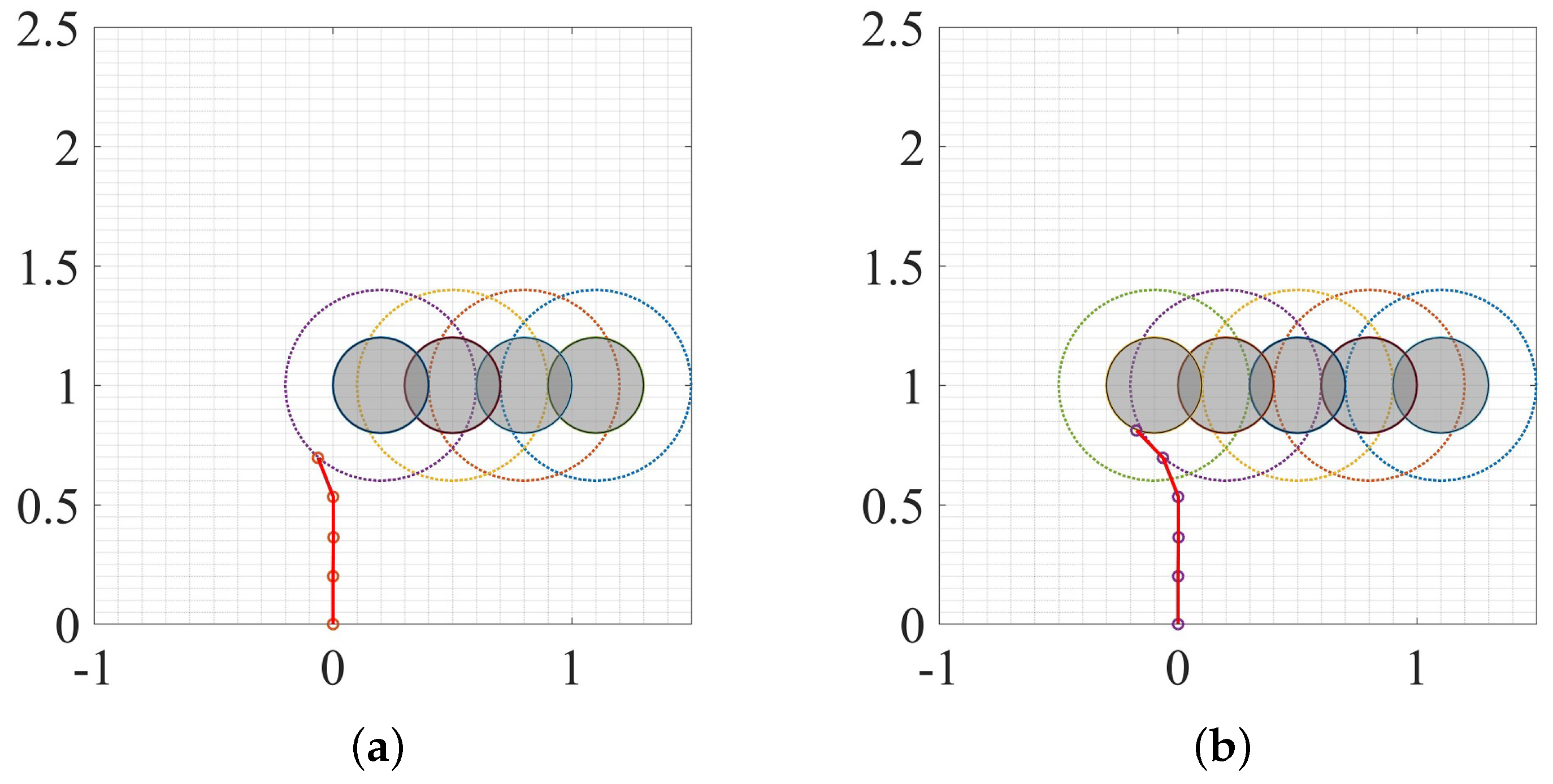
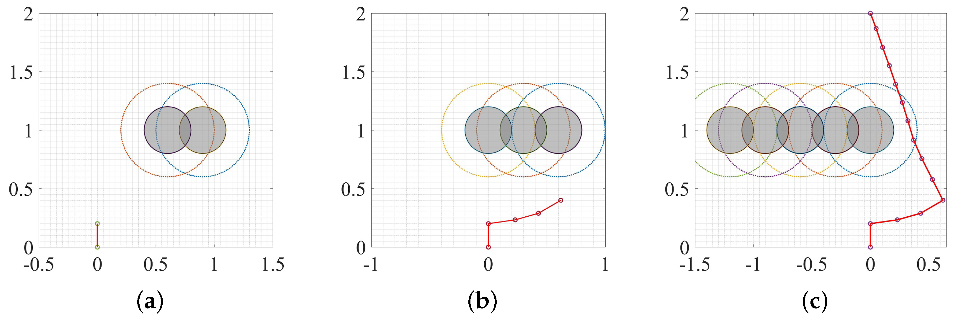
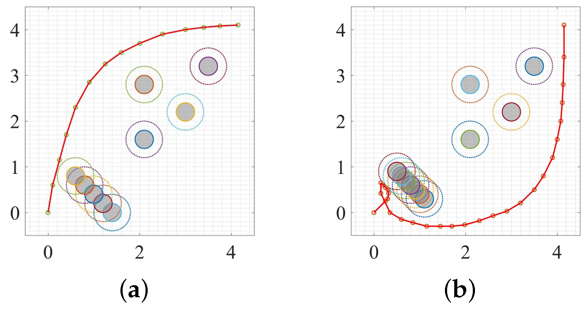
The performance using the DAPF for avoiding the slow and fast obstacles are shown in Figure 7 and Figure 8 respectively. For the slow obstacle, the DAPF has a period of oscillation when the obstacle is in front of the robot. For the fast obstacle, the situation is worse, i.e., the collision between the robot and the obstacle occurs.

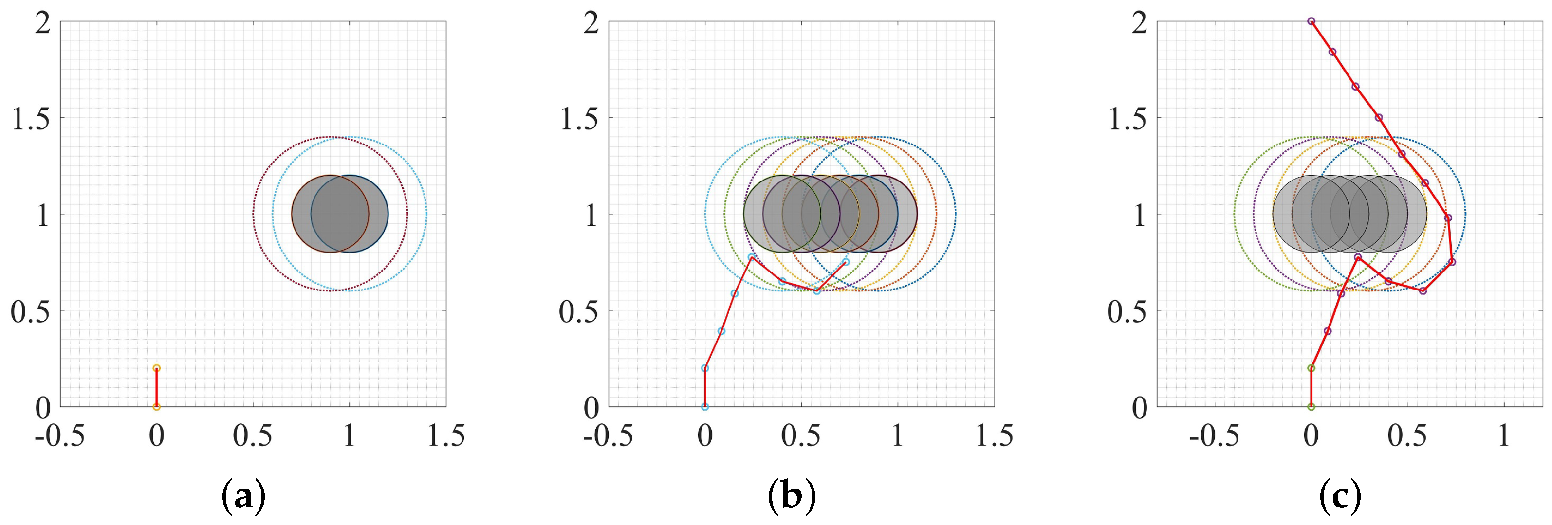
The DVAPF is better than the DAPF as shown in Figure 9 and Figure 10, where we can see that the DVAPF prefers a path behind the moving obstacle. Using such a strategy, the robot and the dynamic obstacle will move in opposite directions when the obstacle enters the robot’s local map if the dynamic obstacle is faster than the robot, and the robot will continue to move towards the target point when $\alpha \in (-\pi ,-\frac{\pi }{2})\cap (\frac{\pi }{2},\pi )$ or the obstacle leaves the robot’s local map. If the moving obstacle is slower than the robot or their velocity is similar, the planned path can be inefficiency and dangerous as shown in Figure 10, i.e., the robot enters the influence area of the obstacle since the robot’s deflection angle is too small to avoid the obstacle.

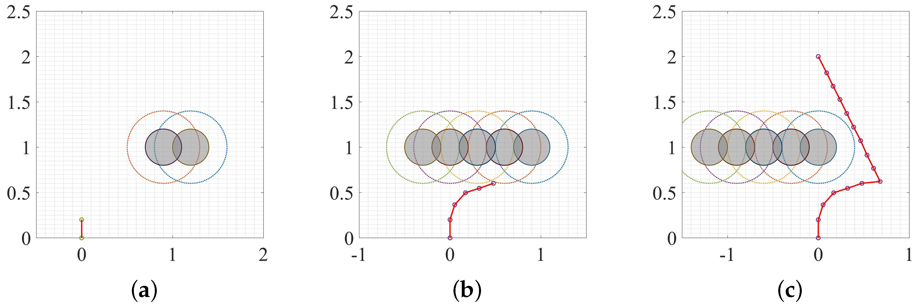
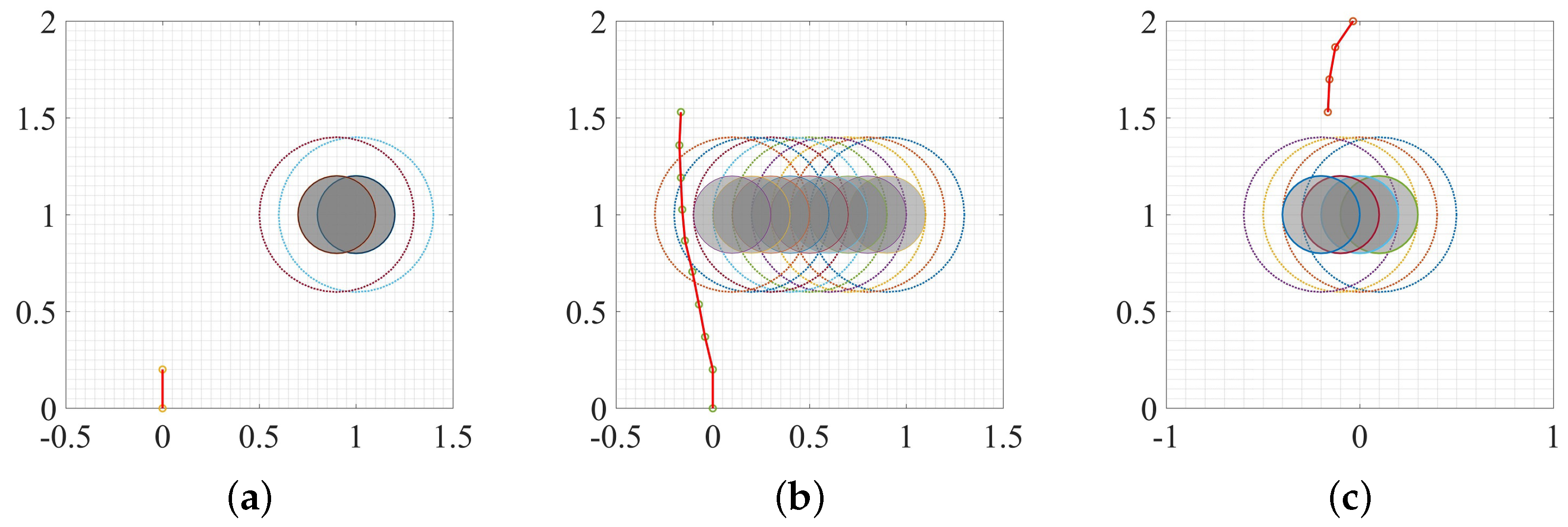
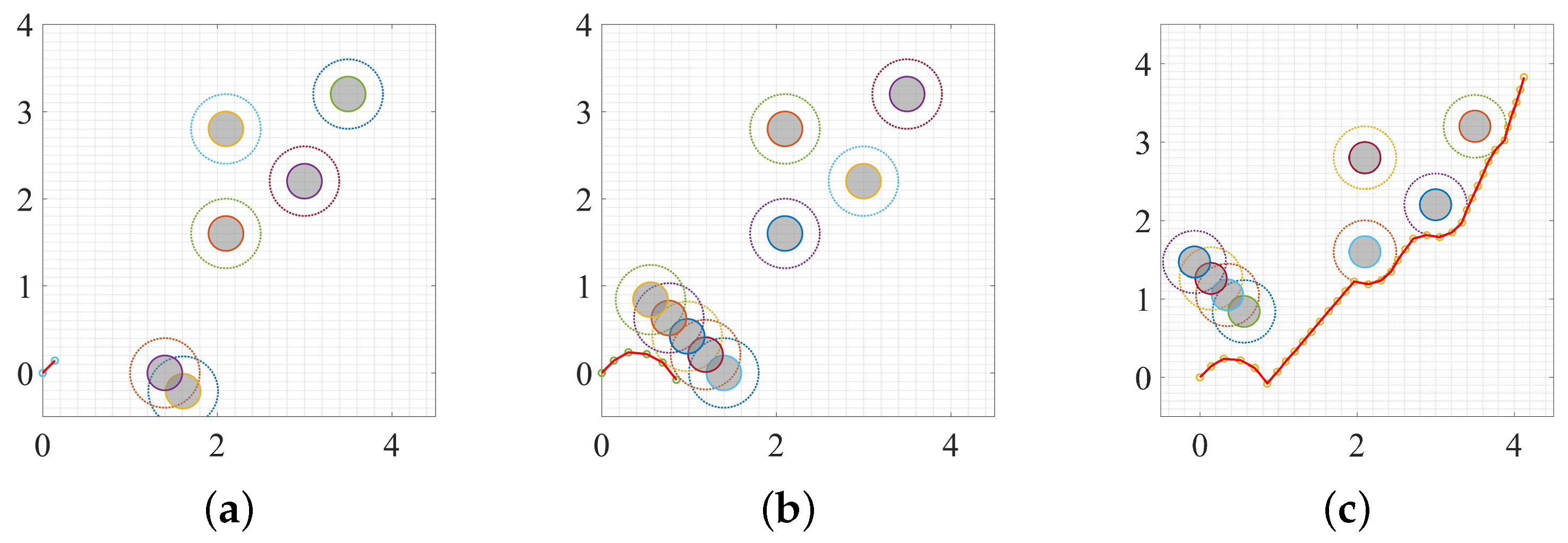
In contrast to the DVAPF and DAPF, the DIAPF has the best performance according to the experiment results as shown in Figure 11 and Figure 12. From the experimental results, it can be seen that the DIAPF approach can make a prediction according to the state of the moving obstacle: if the obstacle velocity is similar or faster, the robot can plan a path behind the obstacle. If the obstacle velocity is slower, the robot can plan a path in front of the obstacle. This strategy makes the planned path more efficient. In addition, the distance influence factor plays a key role to increase the safety and effectiveness of the planned path, e.g., the distance influence factor can reduce the robot’s deviation angle if the moving obstacle is far away, and can increase this angle if the moving obstacle is closer.

3.3. Dynamic Environment

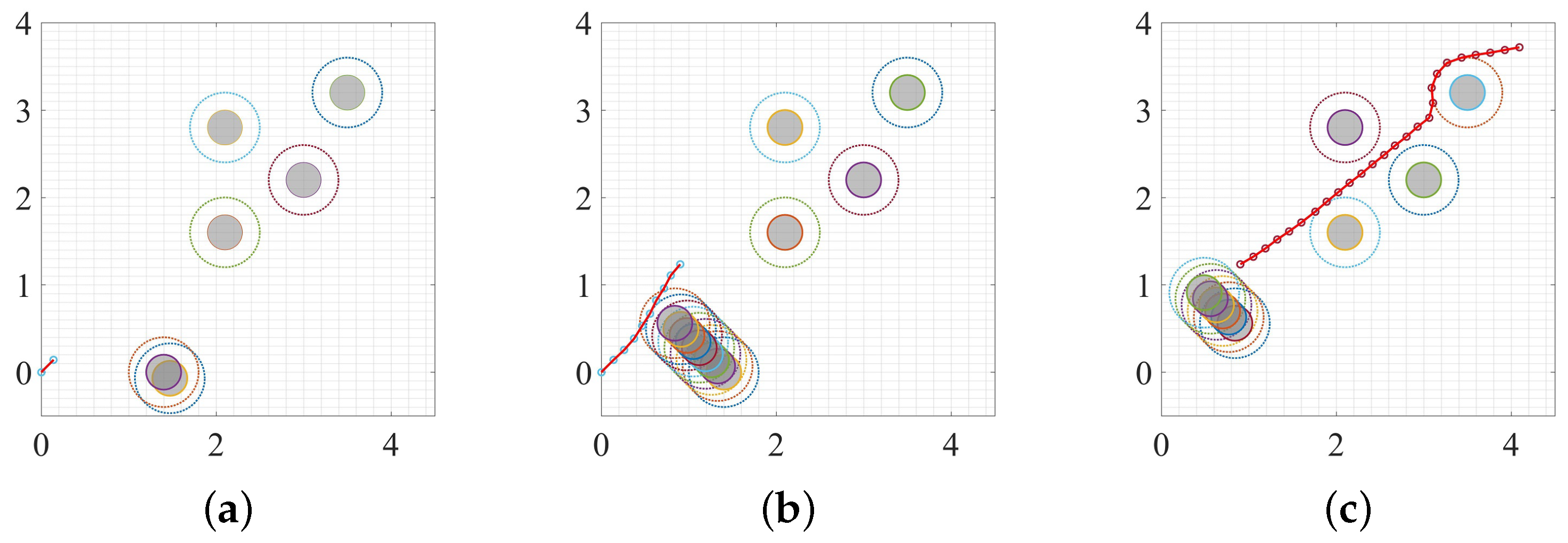
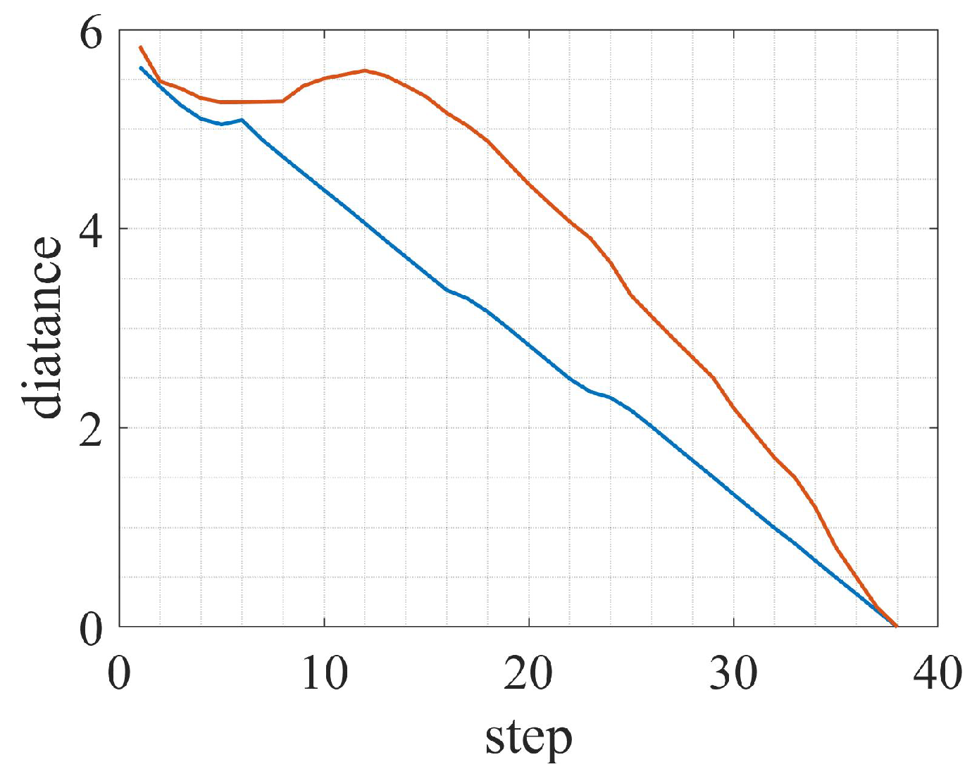
In this section, we compare the proposed DIAPF method to the ROS [26] path plan package which employs the DWA and A* algorithm. The experimental environment includes four static obstacles and a moving obstacle. As can be seen from Figure 13, the ROS uses A* algorithm to plan a global path and uses the DWA algorithm to handle nearby obstacles in the local map. If the speed of the moving obstacle is slow, the robot can avoid the obstacle directly as shown in Figure 13a. However, if the obstacle moves fast, the robot needs to re-plan the path according to the position of the obstacle. The global path also needs to replan according to the local path changes as shown in Figure 13b. In contrast to the ROS method, the proposed DIAPF can make decisions in advance according to the relative velocity between the moving obstacle and robot as shown in Figure 14 and Figure 15. The planned path using the DIAPF is more efficient than the one using the ROS module as seen in Figure 16, which shows the changes of the distance between the robot and the target point. The DIAPF shows a linear decrease of the distance while the ROS shows a curve that decreases first and then increases due to a re-planned path.

4. Conclusions

In this paper, we introduce a dynamic window approach (DWA) and danger index (DI) based artificial potential field (APF) for static and moving obstacle avoidance. The dynamic window approach based APF (DAPF) can overcome the local minimum problem since the DWA can predict the local minima region and avoid in advance. For moving obstacles, we propose a novel danger index based APF (DIAPF) that considers not only the relative distance, but also the relative velocity between the robot and the moving obstacle. In this way, an optimized strategy can be made according to the motion status of the moving obstacle, which leads to a safer and efficient planned path compared to the state-of-the-art works, e.g., ROS path plan module. Finally, we demonstrate the proposed idea in the real environment using the Turtlebot robot, and the experiment results prove our claims. Future work will be extending current work to the environment with an unknown map and multiple randomly moving obstacles.

References

- Rafieisakhaei, M.; Tamjidi, A.; Chakravorty, S.; Kumar, P.R. Feedback motion planning under non-Gaussian uncertainty and non-convex state constraints. In Proceedings of the 2016 IEEE International Conference on Robotics and Automation (ICRA), New York, NY, USA, 15–19 August 2016; pp. 4238–4244. [Google Scholar]
- Al-Sabban, W.H.; Gonzalez, L.F.; Smith, R.N. Wind-energy based path planning for unmanned aerial vehicles using markov decision processes. In Proceedings of the 2013 IEEE International Conference on Robotics and Automation (ICRA), Karlsruhe, Germany, 6–10 May 2013; pp. 784–789. [Google Scholar]
- Sun, W.; van den Berg, J.; Alterovitz, R. Stochastic extended LQR for optimization-based motion planning under uncertainty. IEEE Trans. Autom. Sci. Eng. 2018, 13, 437–447. [Google Scholar] [CrossRef] [PubMed]
- Chi, W.; Wang, C.; Wang, J.; Meng, M.Q. Risk-DTRRT-Based optimal motion planning algorithm for mobile robots. IEEE Trans. Autom. Sci. Eng. 2008, 142–149. [Google Scholar] [CrossRef]
- LaValle, S.M. Rapidly-Exploring Random Trees: A New Tool for Path Planning; TR 98-11, Tech. Rep.; Iowa State University: Ames, IA, USA, 1998. [Google Scholar]
- Kayraki, L.; Svestka, P.; Latombe, J.C.; Overmars, M. Probabilistic roadmaps for path planning in high-dimensional configurations space. IEEE Trans. Robot. Autom. 1996, 12, 566–580. [Google Scholar] [CrossRef]
- Hart, P.E.; Nilsson, N.J.; Raphael, B.A. Formal basis for the heuristic determination of minimum cost paths. IEEE Trans. Syst. Sci. Cybern. 1968, 4, 100–107. [Google Scholar]
- Dijkstra, E.W. A note on two problems in connexion with graphs. Numer. Math. 1959, 1, 269–271. [Google Scholar] [CrossRef] [Green Version]
- Janabi-Sharifi, F.; Vinke, D. Integration of the artificial potential field approach with simulated annealing for robot path planning. In Proceedings of the 8th IEEE International Symposium on Intelligent Control, Chicago, IL, USA, 25–27 August 1993; pp. 539–544. [Google Scholar]
- Lee, S.; Park, J. Cellular robotic collision-free path planning. In Proceedings of the Fifth International Conference on Advanced Robotics’ Robots in Unstructured Environments, Pisa, Italy, 19–22 June 1991; pp. 536–541. [Google Scholar]
- Khatib, O. Real-Time Obstacle Avoidance System for Manipulators and Mobile Robots. In Proceedings of the 1985 IEEE International Conference on Robotics and Automation, St. Louis, MO, USA, 25–28 March 1985; pp. 500–505. [Google Scholar]
- Volpe, R.; Khosla, P. Manipulator control with superquadric artificial potential functions: theory and experiments. IEEE Trans. Syst. Man Cybern. 1990, 20, 1423–1436. [Google Scholar] [CrossRef] [Green Version]
- Mohanty, P.K.; Parhi, D.R. A new hybrid intelligent path planner for mobile robot navigation based on adaptive neuro-fuzzy inference system. Aust. J. Mech. Eng. 2015, 13, 195–207. [Google Scholar] [CrossRef]
- Min, G.P.; Jeon, J.H.; Min, C.L. Obstacle avoidance for mobile robots using artificial potential field approach with simulated annealing. In Proceedings of the 2001 IEEE International Symposium on Industrial Electronics Proceedings, Pusan, Korea, 12–16 June 2001; pp. 1530–1535. [Google Scholar]
- Zhu, Q.; Yan, Y.; Xing, Z. Robot path planning based on artificial potential field approach with simulated annealing. In Proceedings of the Sixth International Conference on Intelligent Systems Design and Applications, Jinan, China, 16–18 October 2006; pp. 622–627. [Google Scholar]
- Doria, N.S.F.; Freire, E.O.; Basilio, J.C. An algorithm inspired by the deterministic annealing approach to avoid local minima in artificial potential fields. In Proceedings of the 2013 16th International Conference on Advanced Robotics (ICAR), Montevideo, Uruguay, 25–29 November 2013; pp. 1–6. [Google Scholar]
- Lee, D.; Jeong, J.; Kim, Y.H.; Park, J.B. An improved artificial potential field method with a new point of attractive force for a mobile robot. In Proceedings of the 2017 2nd International Conference on Robotics and Automation Engineering (ICRAE), Shanghai, China, 29–31 December 2017; pp. 63–67. [Google Scholar]
- Weerakoon, T.; Ishii, K.; Nassiraei, A.A.F. An artificial potential field based mobile robot navigation method to prevent from deadlock. J. Artif. Intell. Soft Comput. Res. 2015, 5, 189–203. [Google Scholar] [CrossRef]
- Kim, Y.H.; Son, W.-S.; Park, J.B.; Yoon, T.S. Smooth path planning by fusion of artificial potential field method and collision cone approach. MATEC Web Conf. 2016, 75, 05004. [Google Scholar] [CrossRef]
- Ge, S.S.; Cui, Y.J. Dynamic motion planning for mobile robots using potential field method. Auton. Robots 2002, 13, 207–222. [Google Scholar] [CrossRef]
- Cao, Q.; Huang, Y.; Zhou, J. An evolutionary artificial potential field algorithm for dynamic path planning of mobile robot. In Proceedings of the 2006 IEEE/RSJ International Conference on Intelligent Robots and Systems, Beijing, China, 9–15 October 2006; pp. 3331–3336. [Google Scholar]
- Montiel, O.; Sepúlveda, R.; Orozco-Rosas, U. Optimal path planning generation for mobile robots using parallel evolutionary artificial potential field. J. Intell. Robot. Syst. 2015, 79, 237–257. [Google Scholar] [CrossRef]
- Fox, D.; Burgard, W.; Thrun, S. The dynamic window approach to collision avoidance. IEEE Robot. Autom. Mag. 1997, 4, 23–33. [Google Scholar] [CrossRef] [Green Version]
- Kulić, D.; Croft, E.A. Safe planning for human-robot interaction. J. Robot. Syst. 2005, 22, 383–396. [Google Scholar] [CrossRef] [Green Version]
- Kulić, D.; Croft, E.A. Affective state estimation for human–robot interaction. IEEE Trans. Robot. 2007, 23, 991–1000. [Google Scholar] [CrossRef]
- Marder-Eppstein, E.; Berger, E.; Foote, T.; Gerkey, B.; Konolige, K. The Office Marathon: Robust Navigation in an Indoor Office Environment. In Proceedings of the 2010 IEEE International Conference on Robotics and Automation (ICRA), Anchorage, AK, USA, 3–7 May 2010; pp. 300–307. [Google Scholar]
Figure 1.
Definition of attractive force and repulsive force in artificial potential field.
Figure 2.
Problems of a traditional artificial potential field (APF): (a) unreachable goals with obstacles nearby (GNRON) and (b) trapped in a local minimum region.
Figure 3.
Robot trajectories simulated by a dynamic window approach (DWA).