SPH Simulation of Hydraulic Jump on Corrugated Riverbeds
by

Shenglong Gu
1,2, 
Fuping Bo
1,2,
Min Luo
3,*, 
Ehsan Kazemi
4, 
Yunyun Zhang
1,2 and
Jiahua Wei
1,2,5 1
State Key Laboratory of Plateau Ecology and Agriculture, Qinghai University, Xining 810016, China
2
School of Water Resources and Electric Power, Qinghai University, Xining 810016, China
3
Zienkiewicz Centre for Computational Engineering, College of Engineering, Swansea University, Swansea SA1 8EN, UK
4
Department of Civil and Structural Engineering, University of Sheffield, Sheffield S1 3JD, UK
5
State Key Laboratory of Hydroscience and Engineering, Tsinghua University, Beijing 100084, China
*
Author to whom correspondence should be addressed.
Appl. Sci. 2019, 9(3), 436; https://doi.org/10.3390/app9030436
Submission received: 20 December 2018
/
Revised: 14 January 2019
/
Accepted: 16 January 2019
/
Published: 28 January 2019
Abstract
:This paper presents a numerical study of the hydraulic jump on corrugated riverbed using the Smoothed Particle Hydrodynamics (SPH) method. By simulating an experimental benchmark example, the SPH model is demonstrated to predict the wave profile, velocity field, and energy dissipation rate of hydraulic jump with good accuracy. Using the validated SPH model, the dynamic evolvement of the hydraulic jump on corrugated riverbed is studied focusing on the vortex pattern, jump length, water depth after hydraulic jump, and energy dissipation rate. In addition, the influences of corrugation height and length on the characteristics of hydraulic jump are parametrically investigated.
1. Introduction
Corrugated riverbed is a new energy dissipater. It is the corrugation-shape base plate of stilling basin. The main corrugation shapes that have recently been studied are sinusoid, triangle, and trapezoid. It is like adding auxiliary energy dissipation structures (such as block, ridges, and tail pier) on the bottom of stilling basin. Essentially, it is a uniform artificially roughed stilling basin base plate which can greatly intensify the turbulence of hydraulic jump as well as reduce the energy carried by water flow. As a result, the energy dissipation structure and riverbed are less scoured or eroded and the energy dissipation rate is raised.
Rajaratnam et al. [1] first proposed the concept of corrugated riverbed stilling basin; they studied the characteristics of hydraulic jump on sinusoidal riverbed and normalized the water-surface profile and flow rate with non-dimensional analysis. Since then, many scholars have conducted experimental research and theoretical analyses on corrugated riverbed. For example, Tokyay et al. [2] found that the energy dissipation rate and hydraulic jump length on sinusoidal riverbed were respectively 6% higher and 35% smaller than those on smooth riverbed; they, through a large amount of experimental data, proved that conjugate depth could be described by a function concerning Froude number; they also pointed out that conjugate depth was slightly affected by corrugation height and length. Izadjoo et al. [3] studied the hydraulic jumps on various trapezoidal riverbeds with 42 groups of tests; they found that the shear force on trapezoidal riverbed was over ten times larger than that on smooth riverbed and the conjugate depth and jump length respectively decreased by 20% and 50%. It indicates that the stilling basin with corrugated riverbed has great potential in energy dissipation. By studying the characteristics of hydraulic jump on sinusoidal riverbed, Abbaspour et al. [4] found that the tail water depth and jump length on sinusoidal riverbed were respectively 20% and about 50% lower than those on smooth bed and the Froude number had a large impact on conjugate depth and jump length. Elsebaie et al. [5] through experiments investigated the characteristics of hydraulic jumps on triangular, trapezoidal, and sinusoidal corrugated riverbeds and compared their energy dissipation rates. Samadi et al. [6] through 42 groups of tests, studied the hydraulic jumps on six triangular riverbeds of different angles and found that the jump length and tail water depth decreased by 54.7% and 25% respectively and the tail water depth was slightly influenced by corrugation height. Based on the experimental results of previous researches on corrugated riverbed of stilling basin, Fu et al. [7] by combining theoretical analysis with the logarithm law of cross-section velocity distribution as well as momentum equation, obtained the theoretical calculation methods for boundary layer, wall surface resistance, conjugate depth, and length of hydraulic jump; they pointed out that wall surface resistance was an important influencing factor which could not be ignored while solving practical problems as it would greatly affect the characteristics of hydraulic jump on corrugated riverbed. The experimental research method, as a major approach for studying hydraulic jump, is often restricted by measuring equipment and methods, and thus is hard to obtain the specific data of physical variables; the theoretical analysis method, based on considerable systems of partial differential equations, has a complex solving process and is hard to get exact solutions.
With the rapid development of computational fluid dynamics, numerical simulation method can record the whole evolution process of a phenomenon and store specific data. It is suitable for the observation of detailed structure and is an effective way for studying complex hydraulic phenomenon. At present, the most widely used numerical simulation method is grid method. For instance, Long et al. [8] simulated the submerged hydraulic jump on smooth riverbed under the steady flow condition. However, this study could only simulate the hydraulic jump with slight change in free surface and failed to trace the development process of hydraulic jump. Cheng et al. [9] introduced the VOF model to trace the free water surface and simulate the hydraulic jumps on corrugated riverbed under five different conditions, and then verified the feasibility of the numerical simulation model. Zhao and Misra [10] investigated the hydraulic jump on smooth riverbed with VOF method and turbulence model. Through numerical method, Abbaspour et al. [11] studied the hydraulic jump on discontinuous open channel, the hydraulic jump on corrugated riverbed, and the submerged hydraulic jump, respectively. Using a VOF model, Wei et al. [12] studied the hydraulic jump characteristics in stilling basins with triangular and sinusoidal riverbeds. By comparing the numerical and experimental results, it was found that the energy dissipation rate was correlated with the Fr number.
In the last decade, another category of numerical methods that get rid of meshes has undergone significant developments. That is the Lagrangian particle method. The most commonly used particle method is the SPH which was initially used in astrophysical simulations [13] and soon afterwards widely applied in continuous solid mechanics [14] and hydromechanics [15] where it matured rapidly. SPH algorithm solves problem domain based on arbitrarily distributed particle frameworks and has unique advantages in dealing with problems such as large deformation, kinematic interface, and free surface. It has been widely used in the hydrodynamic studies on dam break [16] landslide surge [17] multiphase flow [18] and spillway [19] and significant research results have been achieved.
The pioneering study of mesh-free numerical modeling on the hydraulics could be attributed to Gotoh et al. [20] who used the Moving Particle Semi-implicit (MPS) method to compute a turbulent jet. Although the model was not quantitatively validated by the experimental data, the proposed sub-particle scale (SPS) turbulence model and the soluble inflow wall boundary laid a milestone foundation for the numerous follow-on works in SPH turbulence [21,22] and SPH open-channel flows [23,24]. Another category of SPH models commonly used in the flooding hydraulics is based on the solution of Shallow Water Equations (SWEs), i.e., SWE-SPH, which solves the nonlinear SWEs by using the SPH interpolation principles and benchmark works in this field were documented by [25,26].
In aspect of solving the oscillation in pressure field and diminishing difficulty of post-processing many works have been done. The Moving-Least-Squares (MLS) approach was developed by Dilts [27] and applied successfully to solve pressure oscillation by Colagrossi and Landrini [28]. Meringolo et al. [29] used a filtering technique based on Wavelet Transform to remove the acoustic components for solving the problem of pressure oscillation, especially in the violent sloshing flow. Aristodemo et al. [30] also applied the Wavelet Transform technique to horizontal flow around circular cylinders to alleviate numerical noise in the pressure field. Antuono et al. [31] implemented δ+-SPH scheme to simulate the flows past bodies at large Reynolds numbers, whose results showed that it was effective in preventing the onset of tensile instability.
The representative researches on hydraulic jump based on SPH algorithm are as follows. David et al. [32] proposed three solutions to the discrepancies between the SPH simulated wave profile and the practical one (for example, the large fluctuation accompanied by pressure oscillation) and analyzed the feasibilities of the three solutions, through which the numerical model of modified turbulence model VOT(i) was determined and the wave profile and pressure distribution which agreed with the practical situation were obtained. Chern and Syamsuri [33] used SPH method to study the hydraulic jumps on trapezoidal, triangular, and sinusoidal riverbeds. Patrick Jonsson et al. [34] based on SPH method, studied the characteristics of hydraulic jump with periodic boundary. Padova et al. [35] used WCSPH model to simulate the transition from supercritical to subcritical flow at an abrupt drop for obtaining a deeper understanding of the physical features of a flow.
In summary, there have been many experimental and numerical researches carried out on the hydraulic jumps on the corrugated beds. On the other hand, there have been few attempts on the simulation of hydraulic jumps using SPH, mostly investigating the development of boundary condition techniques and validating their models for smooth beds. Despite the importance of the problem, there was only one SPH study on the simulation of hydraulic jumps on the corrugated beds [33]. Acknowledging the value of the work done by Chern and Syamsuri [33], we also study the effects of corrugated beds on the characteristics of hydraulic jumps due to their importance. In the present study, a two-dimensional (2D) SPHysics (http://www.sphysics.org) model, which is based on the Weakly Compressible SPH (WCSPH) method is applied to study the hydraulic jump on corrugated riverbeds and detailed results and discussions on the characteristics of hydraulic jump, such as jump length, jump height and energy dissipation rate are presented, and also the effect of corrugation wave height and length on the hydraulic jump characteristics are parametrically studied. Further details of those effects are presented, while the results are validated by a set of experimental data.
2. SPH Methodology
2.1. Governing Equations and the SPH Formulations
The governing equations of the SPHysics model are the conservation equations of mass and momentum [36], i.e., Navier-Stokes equations, as follows:
where ρ is the density of a fluid, v the particle velocity vector, p is the fluid pressure, is the kinematic viscosity of a fluid, g is the gravity acceleration, and τ is the turbulence stress tensor which is approximated by the SPS model in the present study.
In WCSPH, the fluid is supposed to have weak compressibility. To control the compressibility of fluid, the following equation of state is introduced by Monaghan and Batchelor [37,38,39]:
where , is the initial fluid density whose value is assigned to, 1000 kg/m3, is the sound velocity corresponding to the preset density. The time step of numerical model can be adjusted by altering sound velocity to meet the requirements on compressibility regulation. However, it should be pointed out that the sound velocity cannot be too low; it is required to be 10 times as large as the maximum velocity of fluid at least, so that the weak compressibility condition, in which the change rate of particle density is lower than 1%, can be ensured.
In SPH, the computational domain is discretized by a collection of particles. Each particle has a fixed mass and moves under external forces. The mass as presented in Monaghan [13] and momentum as presented in Dalrymple [40,41] equations are approximated into the discretized form and solved on each particle as follows:
2.2. A Brief Introduction of the parallelSPHysics
Parallel SPHysics is a free open-source SPH code (http://www.sphysics.org) that was released in 2007. It was jointly developed by the researchers at Johns Hopkins University (Baltimore, MD, USA), University of Vigo (Vigo, Spain), University of Manchester (Manchester, UK) and University of Roma La Sapienza (Roma, Italy). The code is programmed in FORTRAN language and is specifically suitable for the free-surface hydrodynamics [42]. In this paper, we use a parallel version of SPHysics, i.e., parallelSPHyphysics [43], to carry out the simulations of spillway flow over a stepped surface. The code has the same SPH numerical schemes as the serial SPHysics code but has been designed to perform simulations with large numbers of particles. The code is parallelized through an MPI formalism, and thus requires the MPICH or OpenMPI to be installed on the parallel machine. More detailed documentations are available from the SPHysics website (http://www.sphysics.org).
3. Benchmark Study
The hydraulic jump on corrugated riverbed is simulated by the present SPH model and compared with the experimental data in Ead and Rajaratnam [1].
3.1. Computational Parameters
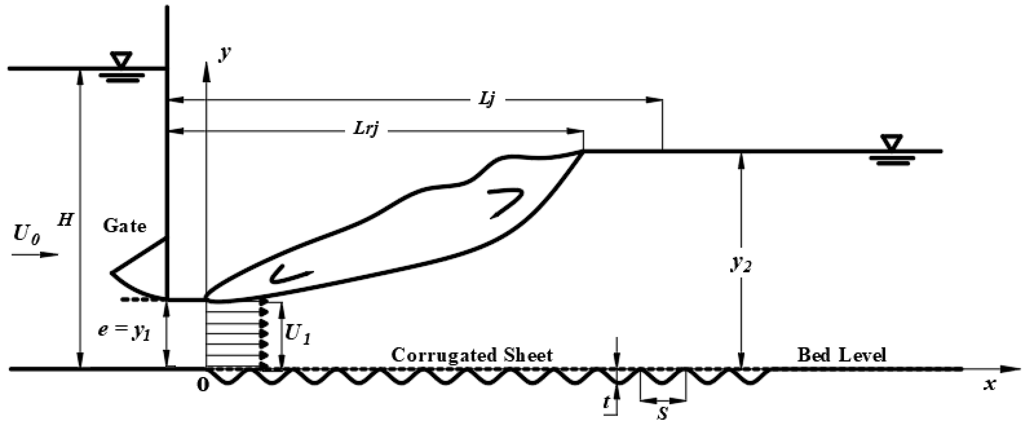
The test model for observing hydraulic jump was a 0.446 m × 0.6 m × 7.6 m rectangular flume made of polymethyl methacrylate whose bottom was installed with aluminum sinusoidal corrugated pipes. As shown in Figure 1, S and t are the corrugation wave length and height of corrugated riverbed, respectively, Fr number is defined by , denotes the cross-section mean velocity before hydraulic jump, q denotes the rate of test flow, and respectively are the water depths before and after hydraulic jump, Lj denotes jump length, and Lrj denotes roller length.
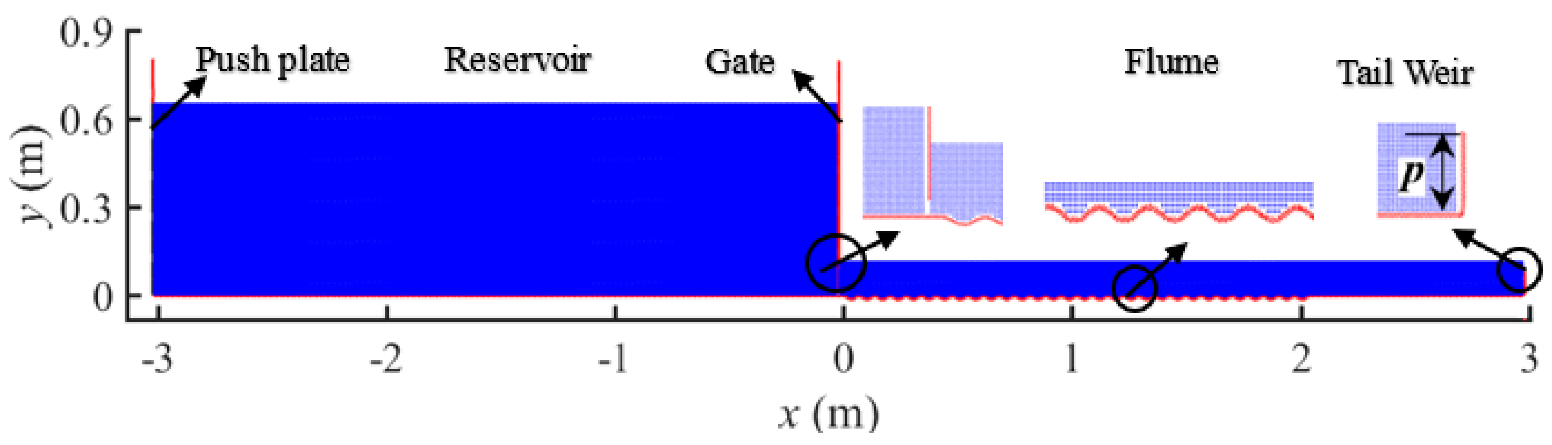
The SPH computational model reproduces the whole experimental setup that includes reservoir, corrugated sheet, gate, and tail weir as shown in Figure 2. Red particles represent the fixed boundary, black particles the moving boundary and blue particles the water particles. The shape of the riverbed corrugation is described by . When the gate height e is constant, the flow velocities of different cases are realized by regulating the water level in the reservoir. The water level is calculated by Equation (6)
where H is the water level of reservoir, is kinetic energy correction factor (under normal flow conditions, ) that considers the water head induced by the water velocity in the reservoir, (= q/H) is the mean water velocity in the reservoir, is the discharge coefficient of gate, ε is the shrinkage coefficient of gate (related to the water depth in and the gate height of the reservoir, and determined according to Table 10-5 as presented in Wen [36]), and 0.95 is assigned to .
A tail weir is set at the end of the flume for controlling tail water, so that the hydraulic jump can form on the corrugated sheet near reservoir gate. The height of the tail weir p is calculated by y2 − h. h is the weir head that can be obtained by solving the equation for the flow rate of sharp-crested weir, i.e., Equation (7) as,
where m0 is calculated by the following empirical formula as
In all the simulations of this study, the quantic spline kernel function is used as presented in Wendland [44]. The MLS density re-initialization scheme is adopted to filter out the numerical noises. The SPS turbulence model is used to consider the fluid turbulence. The solid wall boundaries are modeled by the dynamics boundary condition (DBC) as presented in Dalrymple and Knio [40]. The symplectic (predictor-corrector) scheme is adopted for the time stepping. The time step is determined by the Courant condition as presented in Monaghan and Kos [38]. The initial particle spacing is selected to be , the smoothing length , and the simulation time of each case is 20 s. There is a total number of 96,476 particles in the model of Case A, and among them 4610 are boundary particles. The 6 test cases as presented in Ead and Rajaratnam [1] are studied with the parameters listed in Table 1. The simulations were performed on a cluster at the School of Water Resources and Electric Power, Qinghai University, China, where 32 cores (2 GHz CPU and 32 GB RAM) were used. Depending on the total number of particles for each test case, between 5 and 15 days of CPU time were spent for the computations.
3.2. Flow Rate Through Reservoir Gate
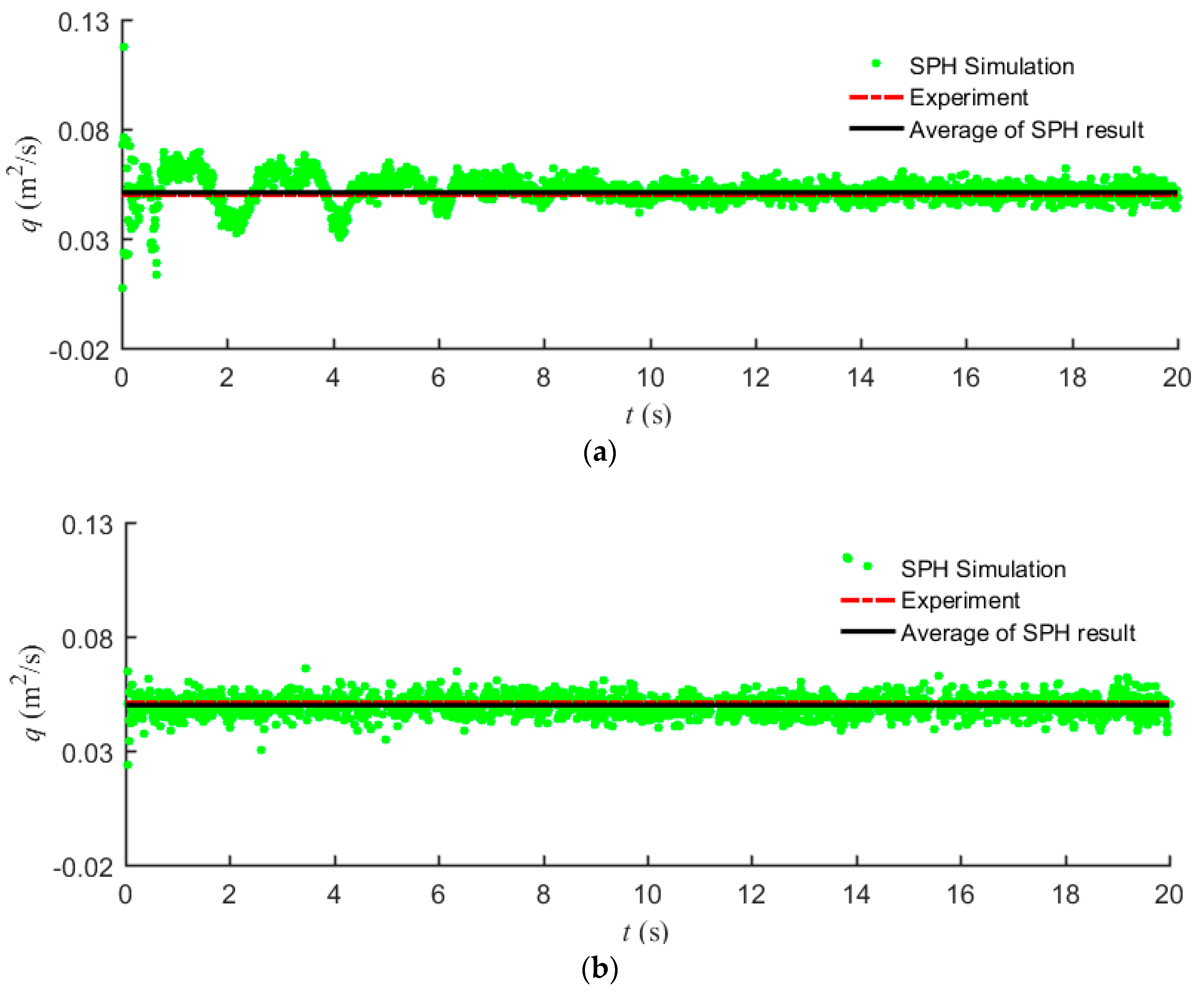
The constant inflow velocities in different cases of this study are obtained by horizontally moving a vertical plate [45] that is installed at the left of the flume. The height of the plate is equal to the water depth H in front of the reservoir gate. The velocity of the plate is equal to the in Equation (6). The rate of the flow through reservoir gate is controlled by the height and velocity of the pushing plate, so that the water level near reservoir gate remains constant and thus the constant flow in the flume can be obtained. The flow rates in the reservoir (the cross-sectional mean flow rate at 0.5 m away from the reservoir gate) and through the reservoir gate of Case A predicted by the SPH model are compared with the experimental results (see Figure 3). The flow rate in the reservoir fluctuates in the first eight seconds and then becomes stable. The standard deviation of the flow rate history is 0.008 m2/s. In addition, it can be seen that the simulated flow rate through the reservoir gate becomes stable very quickly and only shows very minor fluctuation during the whole simulation process. The simulated flow rates in the other cases follow a similar trend in terms of the comparison with the experimental data. For better illustration, the numerical and experimental flow rates through the reservoir gate in all the studied cases are presented in Table 2. The relative deviations between the simulated and experimental flow rates in these cases are from 2.0% to 4.5%. It indicates that the pushing plate model has a good performance in controlling the flow rate and thus the constant inflow condition in the experiment can be simulated.
3.3. Key Features of Hydraulic Jump Evolvement
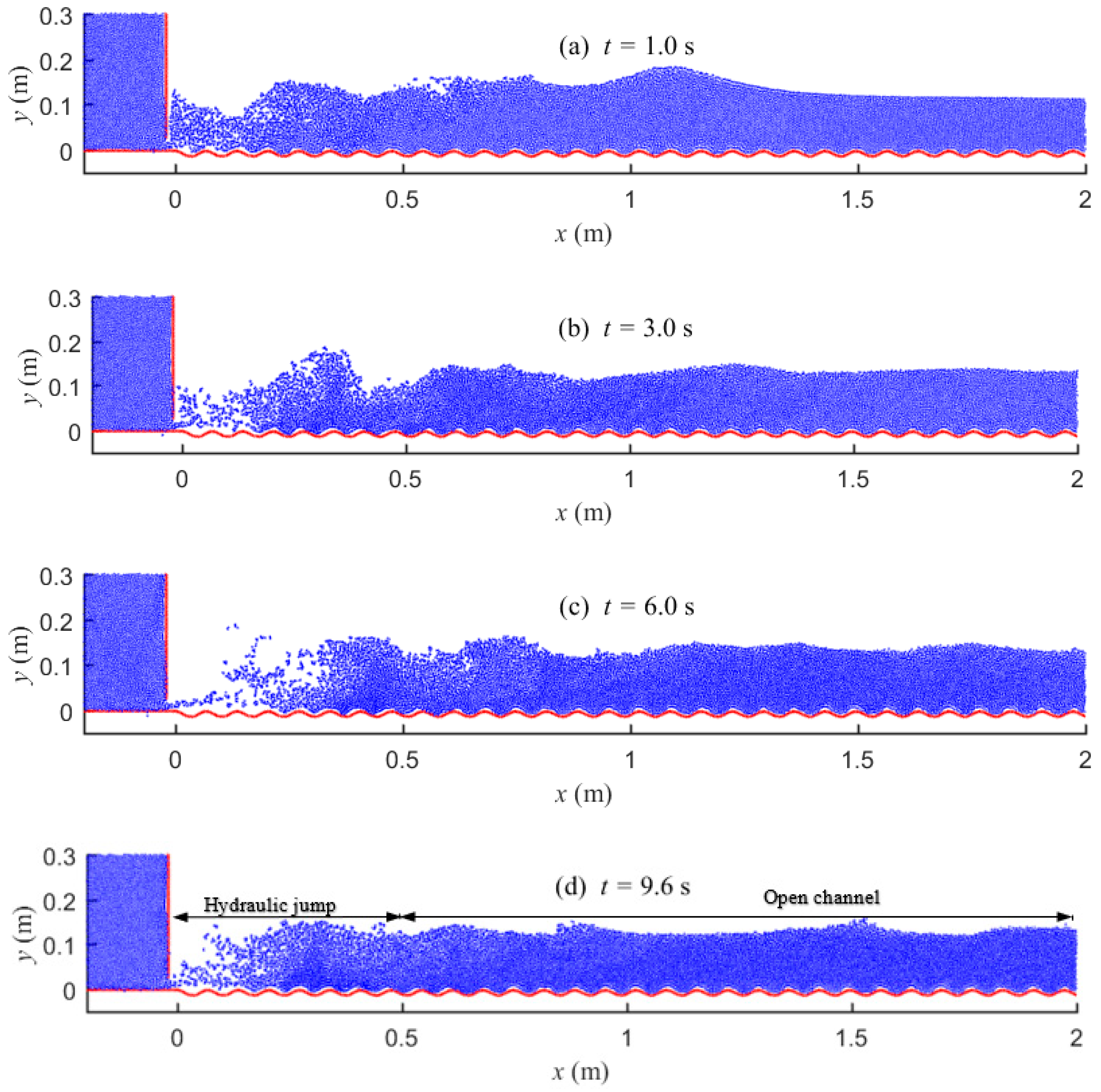
The hydraulic jump in this study is a complicated phenomenon which involves the high-speed jet flow (from the gate), the interaction between the water in the roller area at the top and the mainstream area at the bottom, and the air entrapment. Case A is set as an example to demonstrate the hydraulic jump evolvement. The snapshots at typical instants are presented in Figure 4. When the gate is open, torrents of water gush from the reservoir gate into the flume and violently disturb the slow flow in this region. As the wave propagates, supercritical flow and subcritical flow interact each other, thereby causing the fluctuation of water in the flume, and the fluctuation will propagate to the downstream (t = 1 s). At t = 3.0 s, the hydraulic jump takes the initial shape and forms an evident eddy at the front of the corrugate sheet. The water level will rise again after the downstream flow of the eddy drops. In this way, the high kinetic energy associated with the rapid fluid flow is transformed into potential energy. At around t = 6.0 s, the roller gradually becomes stable and the flow where hydraulic jump occurs can be divided into two parts, i.e., the top flow in the surface roller area and the bottom flow in the mainstream area. In the roller area, the flow is quite fragmentary owing to the addition of considerable bubbles; while in mainstream area below the roller, the water particles are first swirled up to the surface and become a part of the roller and then fall back to the mainstream area, during which, the water particles in the two areas keep exchanging. The hydraulic jump further evolves and becomes stable at around t = 9.6 s. The water surface behind the gate is stable with slight fluctuations. The whole channel can be divided into two parts, namely, the hydraulic jump section where water depth varies and the open-channel section where water depth remains constant.
3.4. Wave Profiles and Velocity Distribution
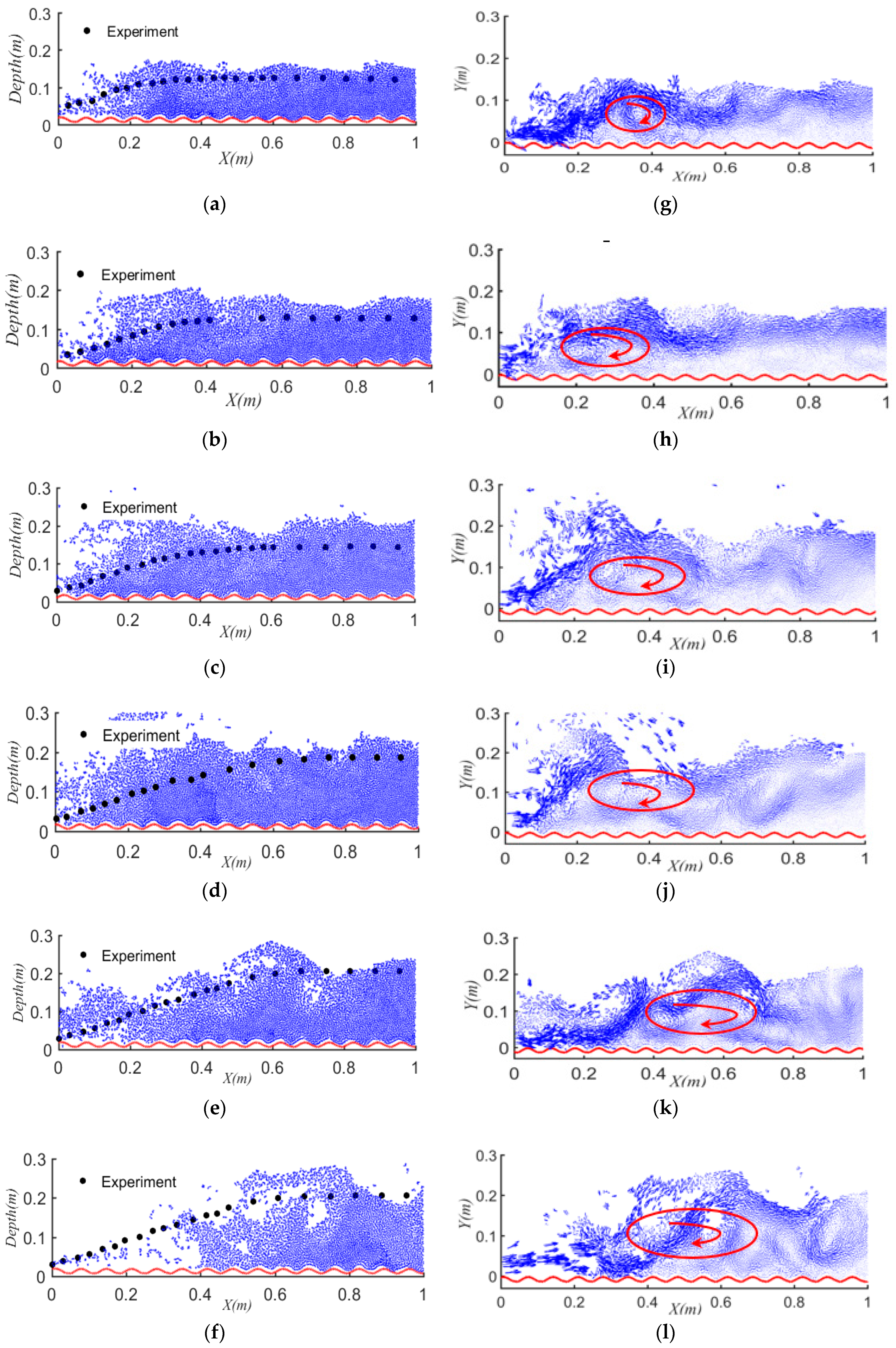
The hydraulic jumps in the other five cases develop in a similar manner as that in Case A. The wave profiles at the steady state in these cases are presented in Figure 5, in which the SPH results are in general good agreement with the laboratory measurement in Ead and Rajaratnam [1]. When the water in the reservoir goes through the gate, rapid flows are generated just downstream of the gate. The wave profiles predicted by SPH in all the cases are disordered. However, the experimental wave profiles published as presented in Ead and Rajaratnam [1] are smooth. In practice, the hydraulic jump contains bubble flows. Thus, the experimental results are interfered owing to the splashing of fragmentary flow caused by the roller. Moreover, the SPH numerical model proposed in this paper does not consider the influence of air on water motion, resulting in the error of results. Consequently, deviations between the experimental and SPH wave profiles exist.
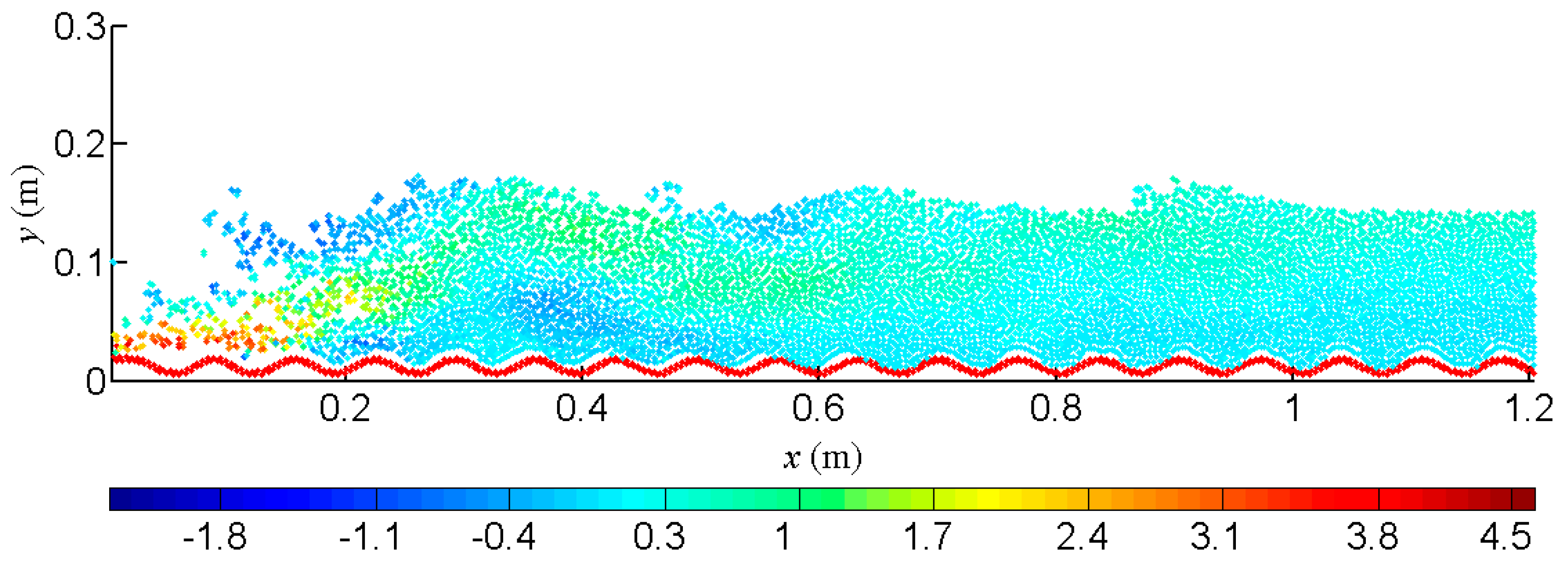
It can be seen from the velocity vectors of Cases A, B, C, and D (Figure 5g–j) that when the corrugation shapes and gate heights e are the same, the flow becomes more fragmentary as the Fr number increases and there is a distinct eddy structure. The formation of roller is mainly caused by the uneven distribution of flow velocity within the hydraulic jump section. The water particles between the flow layers are in relative motion, leading to the generation of internal friction shear stress. In addition, this stress between flow layers is manifested as the downstream flow on the surface and the reverse flow at the bottom, namely, the clockwise roller. Under the same conditions, both the slope and size (see the ellipses in the right column of Figure 5) of the roller increase with the Fr number. It means that the influencing region of roller expands gradually. The contour of the horizontal velocity of Case A is presented in Figure 6. The flows within the hydraulic jump section contain the downstream flow of positive velocity and the reverse flow of negative velocity. The reverse flow mainly exists in the surface and bottom areas. The velocity of flow within the hydraulic jump section differs significantly. Specifically, the flows near the wall and water surface are at low velocity, while the flow in the middle layer is at high velocity. Thus, a torque generates in the hydraulic jump section, manifested as the clockwise roller. In the open channel behind the hydraulic jump section, the flow on the surface has the maximum velocity, while that near the wall has the minimum velocity. The countercurrent near the water surface is caused by the backflow of water, while that at the bottom is mainly resulted from the clockwise roller.
For clarity, the steady-state wave profiles for the six cases are compared in Figure 7, with the result of an error analysis in Table 3. After comparing the wave profiles of Cases A, B, C and D (of the same corrugated riverbed), it is found that when the corrugation shapes and the gate heights are the same, the hydraulic jumps become more violent for higher Fr numbers. The corrugation changes the local fluid motion, which then affects free-surface profile, as can be seen from the comparison between Cases E and F. The relative errors of each case are varied between −9.1% and 9.6%. A more detailed comparison study on the effect of corrugation shape on the hydraulic jump process will be presented in Section 5.
3.5. Jump Length, Water Depth and Energy Dissipation Rate
Jump length, water depth after hydraulic jump, and energy dissipation rate are important indicators for project design. The jump length determines the length of stilling basin, and the water depth after jump determines the height of apron. In practical applications, the stilling basin should be designed to be as short as possible while satisfying the energy dissipation rate to save construction costs.
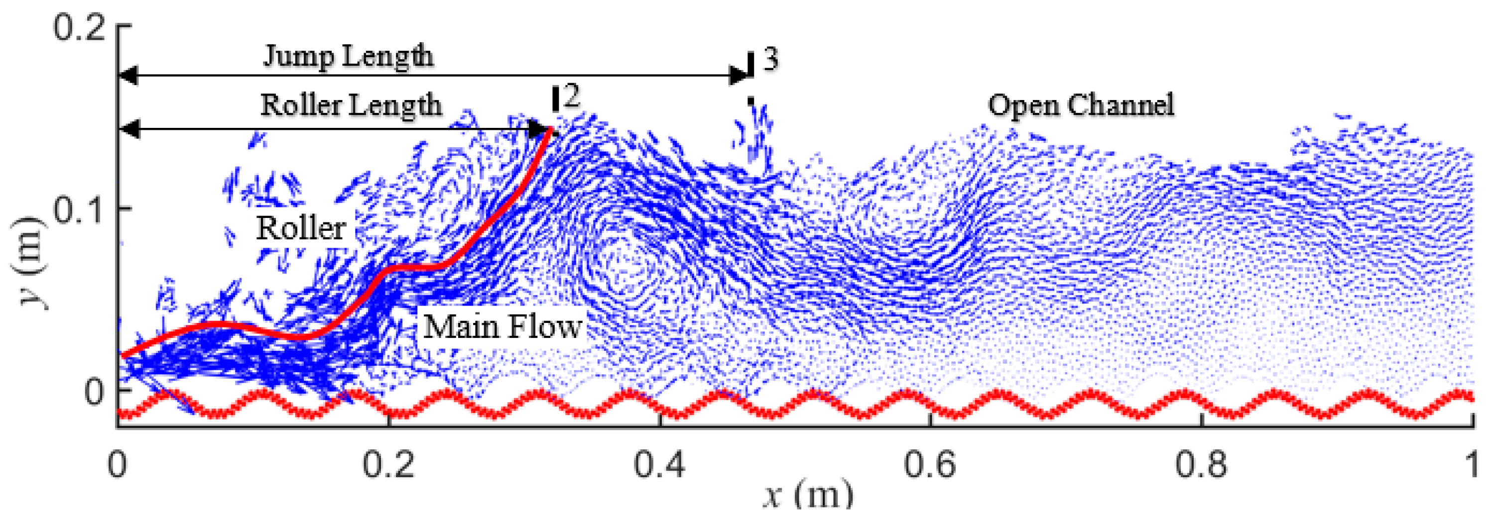
When hydraulic jump occurs, the flow swirls wildly, leading to a dramatic change in the surface water. The water at the end of the roller constantly flows into the mainstream and thus is gradually submerged and finally develops into open-channel flow when the water surface cannot be greatly affected by the swirling vortex. As is shown in Figure 8, the roller length is from the beginning of hydraulic jump to Location 2 (i.e., the end of the roller); the jump length , namely the range of water surface affected by hydraulic jump, is from the beginning of hydraulic jump to Location 3 where the water flows back to the free surface after tumbling over the roller. The experimental and simulated roller lengths () and jump lengths () of the six studied cases as well as the length of hydraulic jump on smooth riverbed () are presented in Table 4. The predicted and by SPH are in good agreement with the experimental results. The maximum relative errors for and are 6.5% and 5.7%, respectively. This shows the good accuracy of the present SPH model. For all the cases, is 30% smaller than , and this number for Case C reaches 40%. It indicates that corrugated sheet can improve energy dissipation rate and reduce jump length as well. In practice, therefore, the length of a stilling basin can be reduced by using corrugated bed.
The water depth at Location 3 in Figure 8 (the starting location of open-channel flow) is considered to be the water depth after hydraulic jump (y2). The experimental and simulated water depths (y2) of the six studied cases as well as the water depth of smooth riverbed case (y2*) are listed in Table 5. The SPH model over predicts the water depth, with the maximum error around 11% in the six cases. The discrepancy is partly attributed to the experimental errors in measuring the energetic free surface of the hydraulic jump. The water depths after hydraulic jump of the six cases with corrugated riverbeds are about 30% smaller than that of the smooth riverbed case.
The hydraulic jump dissipation is one of the major energy dissipation modes of outlet structures. When flow at high velocity discharges into stilling basin, a hydraulic jump occurs, after which, the rapid flow will slow down rapidly, dissipating most of the energy of upstream flow. Figure 9 shows the mean flow velocities () of the studied cases along the channel. In all the cases, the flow has the maximum velocity while passing through the gate (at the beginning of hydraulic jump), and starts to decline progressively thereafter (the decreased amount reaches 85%), and eventually becomes stable in the open-channel region. With the water depths and wave velocities at the reservoir gate and Location 3 in Figure 8, the wave energies at these two locations can be computed by using the formulae as presented in Wen [36]. The difference of these two energies is the energy dissipated by the hydraulic process, which divided by the wave energy at the reservoir gate is the energy dissipation rate η. Energy dissipation rate η on horizontal bed of rectangular channel was computed by the following equations [36].
The η values of Cases A, B, C, and D are presented in Table 6. It can be seen that the current SPH model can predict the energy dissipation rate with generally good accuracy (maximum error of 6%). Within the range of Fr = 4–7, the energy dissipation rate of stilling basin with corrugated riverbed ranges between 45.7% and 67.4%, being around 10% higher than that of smooth riverbed (ranging from 39.2% to 63.4%). Within the studied range of Fr number, the energy dissipation rates of both corrugated riverbeds and smooth riverbed increase with the Fr number.
This section studies the evolution process of hydraulic jump on corrugated riverbed by varying the inflow condition and the corrugation shape. The SPH model can capture the key phenomena in the hydraulic jump development process. The wave profiles, jump lengths, water depths after the hydraulic jump and the energy dissipation rates of the studied cases obtained by the SPH model are in generally good agreement with the experimental results, which demonstrates the accuracy of the SPH model. Using this model, a parametric study on the corrugation shape will be conducted in the next section.
4. Influence of Corrugation Height and Length on Hydraulic Jump
The height and length of corrugation are important design parameters for corrugated riverbeds. In this section, a parametric study is conducted to assess how these two factors affect the wave energy dissipation efficiency. Four corrugation shapes (two corrugation heights and two lengths) are studied. For each corrugation shape, two gate heights and three Fr numbers are tested. There are 24 cases in total, as shown in Table 7. It can be seen that, for the same riverbed, the energy dissipation rate increases with the Fr number. The practical implication is that a corrugation riverbed can dissipate more energy when the upstream dam releases water in which circumstance the inflow to the open channel has a large velocity.
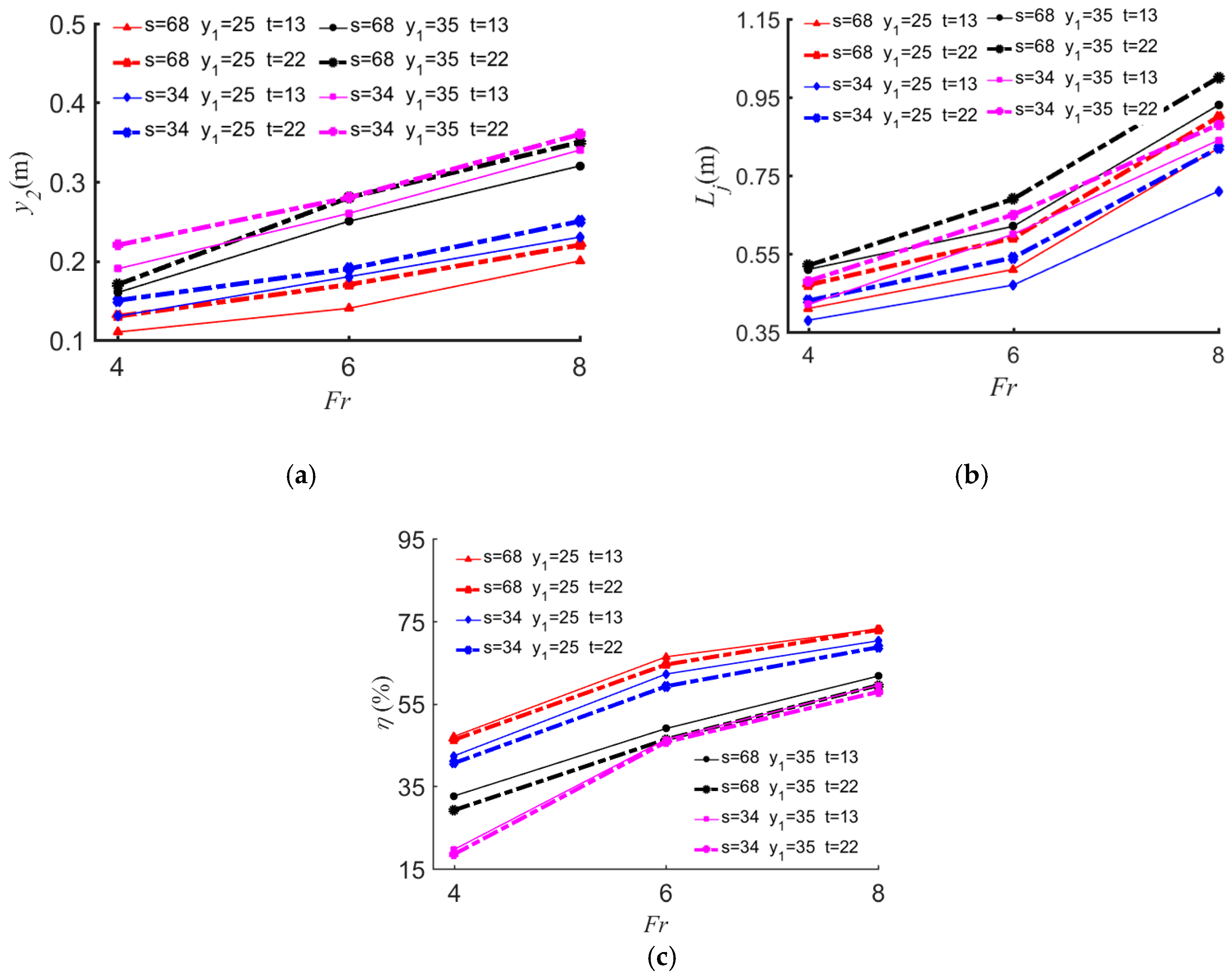
For better illustration, how the water depth (after hydraulic jump), jump length, and energy dissipation rate change with the corrugation wave height and length are shown in Figure 10. When the corrugation height and reservoir gate height remain constant, both the water depth and jump length increase with the corrugation height for all the Fr numbers; yet the corrugation height has a negligible influence on the energy dissipation rate. In addition, it is found that, for the same corrugation shape (S and t fixed), as the reservoir gate height increases, both the water depth after hydraulic jump and the jump length increase significantly, while the energy dissipation rate decreases.
When the corrugation height of the riverbed and the gate height are fixed, the corrugation wave length displays a negative relationship with the water depth after hydraulic jump, i.e., the larger the corrugation length, the smaller the water depth. In practical applications, water depth determines the apron height of a stilling basin. A larger water depth will lead to a higher apron, thereby increasing the construction cost. Therefore, the project cost can be reduced by using riverbed with a reasonably longer corrugation wave length. On the other hand, the jump length increases with the corrugation wave length within a certain range. Increasing the jump length increases the length of the water channel and hence the engineering cost. Considering that a longer corrugation wave length within a certain range can reduce the water depth after hydraulic jump, the effects of corrugation length on the hydraulic jump properties should be comprehensively considered for a cost-effective design. For the energy dissipation rate, it increases with the corrugation length within the range of the present study.
5. Sensitivity Analysis of Computational Resolution
A convergence analysis is performed by changing the initial particle spacing. The simulation of Case A is repeated with flour particle spacings of 0.005, 0.006, 0.008 and 0.01 m, then the errors associated with the discharge and water-surface profiles are computed and compared. Table 8 and Table 9 present the results of this analysis. The results show that the error decreases when a smaller particle spacing (a higher computational resolution) is used. The particle spacing of 0.005 m yields the best accuracy among those four particle spacings. Due to the limitations with the computational time and cost, it was not possible to test particle spacings smaller than 0.005 m. Husain et al. [19] showed that using particle spacings smaller than 0.005 m may enhance the accuracy (which is insignificant), while the increase in the computational time could be outrageous.
6. Conclusions
In the present paper, a 2D SPHysics model is used to simulate the hydraulic jump on corrugated riverbed. Validated by an experimental example, this model is shown to be of general good accuracy in simulating the hydraulic jump process. By using this model, the dynamic evolvement of a hydraulic jump over corrugated riverbed is analyzed by looking into the velocity distribution, jump length, water depth after hydraulic jump, and energy dissipation rate. It is found that a clockwise vortex forms in the hydraulic jump area. For the same corrugation shape, the slope of the vortex roller increases with the Fr number, and so does the influencing region of the vortex. The roller length, jump length, and water depth after hydraulic jump increase with the Fr number. In all the studied cases, the hydraulic jump over corrugated riverbed dissipates over 45% of the wave energy, which is 10% more than that over the smooth riverbed.
A parametric study is conducted to investigate the effect of the corrugation shape on the wave energy dissipation efficiency. It is found that the corrugated riverbed is more effective when the inflow has larger velocity (and hence more wave energy). Within the studied range, the following observations are made: 1) when the corrugation length and the reservoir gate height are fixed, the corrugation height displays a positive correlation with the water depth after hydraulic jump and the jump length, while the corrugation height has an insignificant effect on the energy dissipation rate; and 2) when corrugation height and the reservoir gate height are fixed, the water depth after hydraulic jump reduces as the corrugation length increases, while the jump length and energy dissipation rate increase as the corrugation length increases.
As a further study, by investigating the application of variable smoothing length, the authors aim to enhance the accuracy of the model in the areas with high Fr number, such as the jet at the downstream of the gate where the flow depth is shallow, and the computational resolution is not sufficient to capture the detailed velocity and pressure fields.
Author Contributions
Conceptualization, S.G., F.B. and J.W.; methodology, S.G., F.B. and M.L.; simulation and data analysis, S.G., F.B., M.L., Y.Z. and E.K.; writing—original draft preparation, S.G., F.B. and Y.Z.; writing—review and editing, S.G., F.B., M.L. and E.K.
Funding
This research work is supported by the National Key R&D Program of China (No. 2017YFC0404303), National Natural Science Foundation of China (No.51869025 and No.51479087), Qinghai Science & Technology Projects (No.2018-ZJ-710), High-end Innovative Talent Program of Qinghai Province and the Open Funding SKHL1710 and SKHL1712 from the State Key Laboratory of Hydraulics and Mountain River Engineering in Sichuan University, China.
Acknowledgments
The authors thank Songdong Shao from the University of Sheffield for his constructive comments in the preparation of this manuscript.
Conflicts of Interest
The authors declare no conflict of interest.
References
- Ead, S.A.; Rajaratnam, N. Hydraulic jumps on corrugated beds. J. Hydraul. Eng. 2002, 128, 656–663. [Google Scholar] [CrossRef]
- Tokyay, N.D. Effect of Channel Bed Corrugations on Hydraulic Jumps; Impacts of Global Climate Change. In Proceedings of the World Water and Environmental Resources Congress 2005, Anchorage, AK, USA, 15–19 May 2005; pp. 1–9. [Google Scholar]
- Izadjoo, F.; Shafai-Bejestan, M. Corrugated bed hydraulic jump stilling basin. J. Appl. Sci. 2007, 7, 1164–1169. [Google Scholar]
- Abbaspour, A.; Dalir, A.H.; Farsadizadeh, D. Effect of sinusoidal corrugated bed on hydraulic jump characteristics. J. Hydro-Environ. Res. 2009, 3, 109–117. [Google Scholar] [CrossRef]
- Elsebaie, I.H.; Shabayek, S. Formation of hydraulic jumps on corrugated beds. Int. J. Civil Environ. Eng. IJCEE–IJENS 2010, 10, 37–47. [Google Scholar]
- Samadi-Boroujeni, H.; Ghazali, M.; Gorbani, B. Effect of triangular corrugated beds on the hydraulic jump characteristics. Can. J. Civil Eng. 2013, 40, 841–847. [Google Scholar] [CrossRef]
- Fu, M.H.; Zhang, Z.C.; Liang, F. Test analysis of characteristics of hydraulic jump on corrugated beds of stilling basin. Hydro-Sci. Eng. 2016, 31, 45–49. [Google Scholar]
- Long, D.; Steffler, P.M.; Rajaratnam, N. A numerical study of submerged hydraulic jumps. J. Hydraul. Res. 1991, 29, 293–308. [Google Scholar] [CrossRef]
- Cheng, X.; Chen, Y. Numerical simulation of hydraulic jumps on corrugated beds. J. Hydraul. Eng. 2005, 10, 52–57. [Google Scholar]
- Zhao, Q.; Misra, S.K.; Svendsen, I.A. Numerical study of a turbulent hydraulic jump. In Proceedings of the 17th Engineering Mechanics Conference, Newark, DE, USA, 13–16 June 2004. [Google Scholar]
- Abbaspour, A.; Farsadizadeh, D.; Dalir, A.H. Numerical study of hydraulic jumps on corrugated beds using turbulence models. Turk. J. Eng. Environ. Sci. 2009, 33, 61–72. [Google Scholar]
- Wei, W.; Hong, Y.; Liu, Y. Numerical Simulation on Hydraulic Characteristics of Free Hydraulic Jump on Corrugated Beds of Stilling Basin. J. Syst. Simul. 2017, 29, 918–925. [Google Scholar]
- Monaghan, J.J. Smoothed particle hydrodynamics. Ann. Rev. Astrophys. 1992, 30, 543–574. [Google Scholar] [CrossRef]
- Canelas, R.B.; Crespo, A.J.C.; Dominguez, J.M.; Ferreira, R.M.L.; Gómez-Gesteira, M. SPH-DCDEM model for arbitrary geometries in free surface solid-fluid flows. Comp. Phys. Commun. 2016, 202, 131–140. [Google Scholar] [CrossRef]
- Lind, S.J.; Stansby, P.K.; Rogers, B.D. Incompressible-compressible flows with a transient discontinuous interface using smoothed particle hydrodynamics (SPH). Comput. Phys. 2016, 309, 129–147. [Google Scholar] [CrossRef]
- Albano, R.; Sole, A.; Mirauda, D.; Adamowski, J. Modelling large floating bodies in urban area flash-floods via a Smoothed Particle Hydrodynamics model. J. Hydrol. 2016, 541, 344–358. [Google Scholar] [CrossRef]
- Khayyer, A.; Gotoh, H.; Shao, S.D. Corrected incompressible SPH method for accurate water-surface tracking in breaking waves. Coast. Eng. 2008, 55, 236–250. [Google Scholar] [CrossRef]
- Hu, X.Y.; Adams, N.A. An incompressible multi-phase SPH method. Comput. Phys. 2007, 227, 264–278. [Google Scholar] [CrossRef]
- Husain, S.M.; Muhammed, J.R.; Karunarathna, H.U.; Reeve, D.E. Investigation of pressure variations overstepped spillways using smooth particle hydrodynamics. Adv. Water. Resour. 2014, 66, 52–69. [Google Scholar] [CrossRef]
- Gotoh, H.; Shibahara, T.; Sakai, T. Sub-particle-scale turbulence model for the MPS method–Lagrangian flow model for hydraulic engineering. Comput. Fluid Dyn. 2001, 9, 339–347. [Google Scholar]
- Violeau, D.; Issa, R. Numerical modelling of complex turbulent free-surface flows with the SPH method: An overview. Methods Fluids 2007, 53, 277–304. [Google Scholar] [CrossRef]
- Liu, X.; Lin, P.Z.; Shao, S.D. An ISPH simulation of coupled structure interaction with free surface flows. Fluids Struct. 2014, 48, 46–61. [Google Scholar] [CrossRef]
- Hosseini, S.M.; Feng, J.J. Pressure boundary conditions for computing incompressible flows with SPH. Comput. Phys. 2011, 230, 7473–7487. [Google Scholar] [CrossRef]
- Federico, I.; Marrone, S.; Colagrossi, A.; Aristodemo, F.; Antuono, M. Simulating 2D open-channel flows through an SPH model. Eur. J. Mech. B/Fluids 2012, 34, 35–46. [Google Scholar] [CrossRef]
- Vacondio, R.; Rogers, B.D.; Stansby, P.K. Accurate particle splitting for smoothed particle hydrodynamics in shallow water with shock capturing. Methods Fluids 2012, 69, 1377–1410. [Google Scholar] [CrossRef]
- Chang, T.J.; Chang, K.H. SPH modeling of one-dimensional nonrectangular and nonprismatic channel flows with open boundaries. Hydraul. Eng. 2013, 139, 1142–1149. [Google Scholar] [CrossRef]
- Dilts, G.A. Moving-Least–Squares-Particle Hydrodynamics—I. Consistency and stability. Int. J. Numer. Methods Eng. 1999, 44, 1115–1155. [Google Scholar] [CrossRef]
- Colagrossi, A.; Landrini, M. Numerical simulation of interfacial flows by smoothed particle hydrodynamics. Comput. Phys. 2003, 191, 448–475. [Google Scholar] [CrossRef]
- Meringolo, D.D.; Colagrossi, A.; Marrone, S.; Aristodemo, F. On the filtering of acoustic components in weakly-compressible SPH simulations. J. Fluids Struct. 2017, 70, 1–23. [Google Scholar] [CrossRef]
- Aristodemo, F.; Tripepi, G.; Meringolo, D.D.; Veltri, P. Solitary wave-induced forces on horizontal circular cylinders: Laboratory experiments and SPH simulations. Coast. Eng. 2017, 129, 17–35. [Google Scholar] [CrossRef]
- Sun, P.N.; Colagrossi, A.; Marrone, S.; Antuono, M.; Zhang, A.M. Multi-resolution Delta-plus-SPH with tensile instability control: Towards high Reynolds number flows. Comput. Phys. Commun. 2018, 224, 63–80. [Google Scholar] [CrossRef]
- López, D.; Marivela, R.; Garrote, L. Smoothed particle hydrodynamics model applied to hydraulic structures: A hydraulic jump test case. J. Hydraul. Res. 2010, 48, 142–158. [Google Scholar] [CrossRef]
- Chern, M.J.; Syamsuri, S. Effect of corrugated bed on hydraulic jump characteristic using SPH method. J. Hydraul. Eng. 2012, 139, 221–232. [Google Scholar] [CrossRef]
- Jonsson, P.; Andreasson, P.; Hellström, J.G. Smoothed Particle Hydrodynamic simulation of hydraulic jump using periodic open boundaries. Appl. Math. Model. 2016, 40, 8391–8405. [Google Scholar] [CrossRef]
- De Padova, D.; Mossa, M.; Sibilla, S. SPH Modelling of Hydraulic Jump Oscillations at an Abrupt Drop. Water 2017, 9, 790. [Google Scholar] [CrossRef]
- Wen, D. Engineering Fluid Dynamics. Hydraulics, 3rd ed.; Higher Education Press: Beijing, China, 2010; pp. 1–292. [Google Scholar]
- Monaghan, J.J. Why particle methods work. SIAM J. Sci. Stat. Comput. 1982, 3, 422–433. [Google Scholar] [CrossRef]
- Monaghan, J.J.; Kos, A. Solitary waves on a Cretan beach. J. Waterw. Port. Coast. Ocean Eng. 1999, 125, 145–154. [Google Scholar] [CrossRef]
- Batchelor, G.K. Introduction to Fluid Dynamics; Cambridge University Press: Cambridge, UK, 1974. [Google Scholar]
- Dalrymple, R.A.; Knio, O. SPH modelling of water waves. In Proceedings of the Coastal Dynamics 2001, Lund, Sweden, 11–15 June 2001. [Google Scholar]
- Dalrymple, R.A.; Rogers, B.D. Numerical modeling of water waves with the SPH method. Coast. Eng. 2006, 53, 141–147. [Google Scholar] [CrossRef]
- Gómez-Gesteira, M.; Rogers, B.D.; Crespo, A.J.C.; Dalrymple, R.A.; Narayanaswamy, M.; Dominguez, J.M. SPHysics—Development of a free-surface fluid solver—Part 1: Theory and Formulations. Comput. Geosci. 2012, 48, 289–299. [Google Scholar] [CrossRef]
- Rogers, B.D.; Dalrymple, R.A.; Gómez-Gesteira, M.; Crespo, A.J.C. User Guide for the parallelSPHysics Code Using MPI (Version 2.0); SPHYSICS: Manchester, UK, 2011; Available online: http://www.sphysics.org (accessed on 6 June 2016).
- Wendland, H. Piecewiese polynomial, positive definite and compactly supported radial functions of minimal degree. Adv. Comput. Math. 1995, 4, 389–396. [Google Scholar] [CrossRef]
- Wu, Y. The numerical simulation of stepped spillway based on smoothed particle Hydrodynamics (SPH) method. Master’s Thesis, Qinghai University, Xining, Qinghai, China, 2016. [Google Scholar]
Figure 1.
Schematic view and dimensions of the benchmark example (modified from Figure 1 in Ead and Rajaratnam [1]).

Figure 2.
SPH computational domain of the benchmark example.

Figure 3.
Variation in the flow rate of Case A. (a) Flow rate in the reservoir; (b) Flow rate through the reservoir gate.
Figure 3.
Variation in the flow rate of Case A. (a) Flow rate in the reservoir; (b) Flow rate through the reservoir gate.

Figure 4.
Snapshots of hydraulic jump evolvement.

Figure 5.
Wave profiles and velocity vector of different cases. (a) Wave profile of Case A; (b) Wave profile of Case B; (c) Wave profile of Case C; (d) Wave profile of Case D; (e) Wave profile of Case E; (f) Wave profile of Case F; (g) Velocity vector of Case A; (h) Velocity vector Case B; (i) Velocity vector of Case C; (j) Velocity vector of Case D; (k) Velocity vector of Case E; (l) Velocity vector of Case F.

Figure 6.
Contour of horizontal velocity of Case A.

Figure 7.
Wave profiles of Cases A to F.

Figure 8.
Definitions of roller length and jump length.

Figure 9.
Mean flow velocity of Cases A–F along the channel.

Figure 10.
Water depth after hydraulic jump, jump length, and energy dissipation rate vary with corrugation height. (a) Water depth after hydraulic jump; (b) jump length; (c) energy dissipation rate.
Figure 10.
Water depth after hydraulic jump, jump length, and energy dissipation rate vary with corrugation height. (a) Water depth after hydraulic jump; (b) jump length; (c) energy dissipation rate.


Table 1.
Parameters of the numerical cases.
| Cases | S (mm) | t (mm) | Fr | U1 (m/s) | q (m2/s) | y1 (mm) | y2 (m) | Lj (m) |
|---|---|---|---|---|---|---|---|---|
| A | 68 | 13 | 4 | 2 | 0.051 | 25.4 | 0.104 | 0.41 |
| B | 68 | 13 | 5 | 2.5 | 0.063 | 25.4 | 0.128 | 0.48 |
| C | 68 | 13 | 6 | 3 | 0.076 | 25.4 | 0.145 | 0.54 |
| D | 68 | 13 | 7 | 3.49 | 0.089 | 25.4 | 0.188 | 0.75 |
| E | 68 | 13 | 4 | 2.82 | 0.143 | 50.8 | 0.21 | 0.88 |
| F | 68 | 22 | 4 | 2.82 | 0.143 | 50.8 | 0.21 | 0.88 |
Table 2.
SPH flow rates through reservoir gate in comparison with experimental data.
| Cases | A | B | C | D | E | F |
|---|---|---|---|---|---|---|
| Experiment (m2/s) | 0.051 | 0.063 | 0.076 | 0.089 | 0.143 | 0.143 |
| Simulation (m2/s) | 0.05 | 0.061 | 0.072 | 0.093 | 0.147 | 0.147 |
| Deviation (%) | 2.0 | 3.2 | 3.9 | −4.5 | −2.8 | −2.8 |
Table 3.
Wave profiles comparison with the experimental data.
| Case | A | B | C | D | E | F |
|---|---|---|---|---|---|---|
| Mean Absolute Deviation (10−2 m) | 0.79 | 0.71 | 1.25 | 1.10 | 0.94 | 1.46 |
| Relative Error (%) | 3.54 | −3.90 | −9.10 | 9.60 | 0.84 | −9.10 |
| Root Mean Squared Error (10−2 m) | 0.91 | 0.91 | 1.39 | 1.38 | 1.19 | 1.72 |
Table 4.
Roller lengths and jump lengths of Cases A–F.
| Case | Lrj | Lj | Lj* 1 | ||||
|---|---|---|---|---|---|---|---|
| Experiment | Simulation | Error (%) | Experiment | Simulation | Error (%) | ||
| A | 0.31 | 0.33 | 6.45 | 0.41 | 0.43 | 4.88 | 0.56 |
| B | 0.41 | 0.43 | 4.88 | 0.48 | 0.49 | 2.08 | 0.72 |
| C | 0.48 | 0.46 | −4.17 | 0.54 | 0.52 | −3.7 | 0.9 |
| D | 0.61 | 0.59 | −3.28 | 0.75 | 0.74 | −1.33 | 1.07 |
| E | 0.75 | 0.71 | −5.33 | 0.88 | 0.93 | 5.68 | 1.12 |
| F | 0.61 | 0.63 | 3.28 | 0.82 | 0.85 | 3.66 | 1.12 |
1Lj* computed by Equations (10–57) as presented in Wen [36].
Table 5.
Water depths of Cases A–D after hydraulic jump.
| Case | y2 | y2* | ||
|---|---|---|---|---|
| Experiment | Simulation | Error (%) | ||
| A | 0.104 | 0.112 | 7.69 | 0.132 |
| B | 0.128 | 0.134 | 4.69 | 0.167 |
| C | 0.145 | 0.161 | 11.03 | 0.203 |
| D | 0.188 | 0.191 | 1.6 | 0.239 |
Table 6.
Energy dissipation rates of Cases A–D.
| Case | Fr Number | Corrugated Bed η (%) | Smooth Bed η (%) | ||
|---|---|---|---|---|---|
| Experiment | Simulation | Error (%) | |||
| A | 4 | 49.32 | 46.57 | −5.58 | 39.22 |
| B | 5 | 59.22 | 57.76 | −2.47 | 48.55 |
| C | 6 | 67.18 | 64.42 | −4.11 | 56.05 |
| D | 7 | 68.48 | 67.36 | −1.64 | 63.43 |
Table 7.
Model parameters.
| S (mm) | t (mm) | y1 (mm) | Fr | y2 (m) | Lj (m) | η (%) | S (mm) | t (mm) | y1 (mm) | Fr | y2 (m) | Lj (m) | η (%) |
|---|---|---|---|---|---|---|---|---|---|---|---|---|---|
| 68 | 13 | 25 | 4 | 0.11 | 0.41 | 47.1 | 34 | 13 | 25 | 4 | 0.13 | 0.38 | 42.36 |
| 6 | 0.14 | 0.51 | 66.4 | 6 | 0.18 | 0.47 | 62.19 | ||||||
| 8 | 0.20 | 0.82 | 73.1 | 8 | 0.23 | 0.71 | 70.24 | ||||||
| 35 | 4 | 0.16 | 0.51 | 32.6 | 35 | 4 | 0.19 | 0.42 | 19.67 | ||||
| 6 | 0.25 | 0.62 | 49 | 6 | 0.26 | 0.60 | 46.36 | ||||||
| 8 | 0.32 | 0.93 | 61.7 | 8 | 0.34 | 0.84 | 59.46 | ||||||
| 22 | 25 | 4 | 0.13 | 0.47 | 46.3 | 22 | 25 | 4 | 0.15 | 0.43 | 40.61 | ||
| 6 | 0.17 | 0.59 | 64.5 | 6 | 0.19 | 0.54 | 59.23 | ||||||
| 8 | 0.22 | 0.90 | 72.9 | 8 | 0.25 | 0.82 | 68.67 | ||||||
| 35 | 4 | 0.17 | 0.52 | 29.2 | 35 | 4 | 0.22 | 0.48 | 18.53 | ||||
| 6 | 0.28 | 0.69 | 46.4 | 6 | 0.28 | 0.68 | 45.72 | ||||||
| 8 | 0.35 | 1.00 | 59.5 | 8 | 0.36 | 0.88 | 57.86 |
Table 8.
Discharge deviation with different particle spacing.
| Particle Spacing (m) | Experimental Discharge (m2/s) | SPH-Estimated Discharge (m2/s) | Deviation (%) |
|---|---|---|---|
| 0.005 | 0.051 | 0.05 | 2 |
| 0.006 | 0.051 | 0.052 | −2 |
| 0.008 | 0.051 | 0.049 | 3.9 |
| 0.01 | 0.051 | 0.044 | 13.7 |
Table 9.
Errors of the SPH-estimated water-surface profiles with respect to the experimental data.
| Particle Spacing (m) | Mean Absolute Deviation (10−2 m) | Relative Error (%) | Root Mean Squared Error (10−2 m) |
|---|---|---|---|
| 0.005 | 0.79 | 3.54 | 0.91 |
| 0.006 | 3.14 | −11.12 | 3.65 |
| 0.008 | 2.12 | −14.32 | 2.29 |
| 0.01 | 2.57 | −24.6 | 2.82 |
© 2019 by the authors. Licensee MDPI, Basel, Switzerland. This article is an open access article distributed under the terms and conditions of the Creative Commons Attribution (CC BY) license (http://creativecommons.org/licenses/by/4.0/).
Share and Cite
MDPI and ACS Style
Gu, S.; Bo, F.; Luo, M.; Kazemi, E.; Zhang, Y.; Wei, J. SPH Simulation of Hydraulic Jump on Corrugated Riverbeds. Appl. Sci. 2019, 9, 436. https://doi.org/10.3390/app9030436
AMA Style
Gu S, Bo F, Luo M, Kazemi E, Zhang Y, Wei J. SPH Simulation of Hydraulic Jump on Corrugated Riverbeds. Applied Sciences. 2019; 9(3):436. https://doi.org/10.3390/app9030436
Chicago/Turabian StyleGu, Shenglong, Fuping Bo, Min Luo, Ehsan Kazemi, Yunyun Zhang, and Jiahua Wei. 2019. "SPH Simulation of Hydraulic Jump on Corrugated Riverbeds" Applied Sciences 9, no. 3: 436. https://doi.org/10.3390/app9030436
Note that from the first issue of 2016, this journal uses article numbers instead of page numbers. See further details here.