Feature Weighting Based on Inter-Category and Intra-Category Strength for Twitter Sentiment Analysis

1
College of Information and Communication Engineering, Sungkyunkwan University, Suwon 440-746, Korea
2
College of Software, Sungkyunkwan University, Suwon 440-746, Korea
*
Author to whom correspondence should be addressed.
Appl. Sci. 2019, 9(1), 92; https://doi.org/10.3390/app9010092
Submission received: 3 December 2018
/
Revised: 19 December 2018
/
Accepted: 22 December 2018
/
Published: 27 December 2018
(This article belongs to the Section Computing and Artificial Intelligence)
Abstract
:The rapid growth in social networking services has led to the generation of a massive volume of opinionated information in the form of electronic text. As a result, the research on text sentiment analysis has drawn a great deal of interest. In this paper a novel feature weighting approach is proposed for the sentiment analysis of Twitter data. It properly measures the relative significance of each feature regarding both intra-category and intra-category distribution. A new statistical model called Category Discriminative Strength is introduced to characterize the discriminability of the features among various categories, and a modified Chi-square (χ2)-based measure is employed to measure the intra-category dependency of the features. Moreover, a fine-grained feature clustering strategy is proposed to maximize the accuracy of the analysis. Extensive experiments demonstrate that the proposed approach significantly outperforms four state-of-the-art sentiment analysis techniques in terms of accuracy, precision, recall, and F1 measure with various sizes and patterns of training and test datasets.
1. Introduction
Recently, exponential growth of the Internet has spurred the usage of information in diverse formats [1]. Especially, social networking services (SNS) such as Twitter provide users with a platform for presenting their preferences and opinions on various topics. Such opinionated textual information has become a gold mine for the institutions and companies in understanding the users’ sentiments regarding their products and services [2,3]. Sentiment analysis refers to a research field of automatic language processing, which extracts and analyzes the opinions, sentiments, and subjectivities from the text [4]. It has drawn increasing interest, and become an active research topic due to the importance of satisfying the emerging demands [5]. Text categorization (TC) is the task of effectively organizing a massive amount of data, which is commonly employed for sentiment analysis [6].
TC is the process of automatically classifying each piece of the text in the form of a document into predefined category [6]. Generally, it consists of four stages: processing, document representation, feature selection and weighting, and finally classification. In the processing stage, the basic language processes such as tokenization and stop-word removal are performed to normalize the text. For the document representation, the Vector Space Model (VSM) is the most commonly used method, wherein the documents are represented as vectors in the feature space. In feature selection and weighting, a filtering technique based on Chi-square statistics, mutual information, or information gain is employed to extract a set of useful features from the feature space [7]. Also, a weight is assigned to each term (feature), which is decided according to its importance. Finally, a classification algorithm such as Naïve-Bayes, Decision Tree, or Support Vector Machine is used to classify the tested document into a predefined category [6]. There exist some issues confronting TC. The first issue is how to effectively select useful features from the feature space. As the training data are usually massive, reducing the dimension of the feature space contributes to the saving of a significant amount of computational cost. The second one is the decision of feature weight. Debole [8] firstly proposed the notion of Supervised Term Weighting (STW), where the terms are weighted considering the information of the category of the training dataset [9]. Unlike feature selection, where all the selected features are treated equally, the importance of the features serves as a criterion for determining the weights of the features.
Extensive studies have been conducted for feature weighting with TC, while the method based on the Document Frequency (DF) is the simplest one. It is effective with large-scale corpus due to the simplicity, but overemphasizes the role of the appearance of the terms in deciding the weights, and ignores the terms of multiple appearances. With Term Frequency (TF), a weight is assigned to each term based on its frequency in the document instead of binary representation. With DF and TF, the importance of the terms is measured based on the appearance and frequency, respectively, which are the basic factors employed by various existing feature weighting approaches. Term Frequency and Inverse Document Frequency (TF-IDF) [2] reflects the two factors in deciding the weights to achieve good performance in various situations, and it is therefore widely used. Part-of-Speech feature-based Weighting (PSW) [10] is a recently introduced method that aggregates the terms into groups and weighs them in accordance with their inter-group importance. It performs well in many cases of sentiment analysis, while the clustering strategy significantly affects the performance.
Although numerous schemes exist on feature weighting for sentiment analysis, efficient and accurate decision of the weights of the features according to their importance is still a big issue. In this paper, a novel approach is proposed that explores the intrinsic information of the feature from the initial corpus for deciding the weights [9]. The main contributions of this paper are summarized as follows.
- A novel mathematical model called Category Discriminative Strength (CDS) is proposed, which measures the strength of the terms in differentiating the categories. Also, the Intra-Distribution Measure (IDM) is introduced to characterize the partial significance of the terms inside a category.
- A modified Chi-square statistics model is introduced to measure the intra-category dependency of the features.
- A fine-grained feature clustering strategy is presented, which properly defines the margin of discriminative features and aggregates the features of similar distributions for efficient feature weighting.
- An adaptive weighting strategy is proposed to properly decide the weight of each feature, and the inter-category and intra-category relevance of the features are included to maximize the efficiency of the weighting.
An extensive experiment demonstrates that the proposed approach is superior to the existing state-of-the-art schemes in terms of classification accuracy, precision, recall, and F1 measure. The rest of the paper is organized as follows. Section 2 discusses the background of sentiment analysis. In Section 3 the proposed scheme is presented, and Section 4 shows the results of the experiment with the proposed scheme. Finally, the paper is concluded in Section 5.
2. Related Work
2.1. Twitter Sentiment Analysis and Opinion Mining
Twitter is the most popular microblogging platform allowing the users to create 140-character long text messages called “tweets”. A tweet is a kind of opinionated message expressing the feelings or opinions of the users on the subject. Several millions of active users send and receive over 500 million messages daily [11], which are mixed with various web services such as instant messaging, etc. [12]. Twitter has become a gold mine, and the collection of tweets extracted from the Twitter API has become a source corpus for sentiment analysis [13]. The objective of sentiment analysis is to predict the polarity (positive/negative) of an opinionated piece of text to evaluate the mood of people concerning a particular topic [14]. The lexicon-based approach and machine learning-based approach are the two main approaches that have been adopted for sentiment analysis. The lexicon-based approach uses a sentiment lexicon to analyze the sentiment of tested instances, while the machine learning-based approach employs a machine learning algorithm to train a text classifier for the classification.
Opinion mining is a domain of natural language processing, computational linguistics, and text mining associated with the computational learning of opinions, sentiments, and emotions from the text [12]. The emotion-based views, thoughts, or attitudes toward particular entities is often known as sentiment; hence, opinion mining is also regarded as sentiment analysis. Opinion mining has various applications in the field of education, research, and marketing, etc. For example, it can be used to evaluate the feedback from the customers on the product advertisement, and helps the marketers find out what products or services are popular. Previously, the research studies on opinion mining were not extensive, owing to limited amount of the information people generated. However, massive volumes of opinionated information have become available these days with the rapid growth of various SNS.
2.2. Lexicon-Based Approach
The lexicon-based approach is based on the unsupervised learning technique where a sentiment lexicon is constructed to determine the polarity of the given text via the predefined function of the indicator of positive and negative [15]. The popular lexicons include the Opinion Lexicon [16], AFINN Lexicon [17], and NRC Emotion Lexicon [18]. The value averaging the polarities derived from each word of the text in the lexicon serves as the sentiment score, which reflects the orientation of the polarity of the text [19]. The existing studies generally utilize the polarity of the previous sentence as a tie-breaker when the classification of tested sentences cannot be derived from the scoring function. Therefore, the generation of a meaningful lexicon based on the unsupervised labeling corpus is crucial with the lexicon-based approach [15]. As the creation of a lexicon is a time-consuming process, and a predesigned lexicon is not necessarily directly applicable to different domains and languages, the conventional lexicon-based methods are dedicated to extracting domain-specific words [20].
Extensive researches have been made with the lexicon-based approach. In [21], a visual framework, EmoWeb, was proposed to dynamically analyze the sentiment of textual content relying on a well-constructed lexicon. Experiments were conducted by collecting data from websites to show the applicability of the proposed scheme. A Neural Network (NN) technique was used to overcome the shortcoming of the lexicon-based approach, where some words are ignored by the lexicon [22]. A Portuguese context-sensitive lexicon [23] was constructed for sentiment polarity identification. It employed LexReLi as methodology to build the proposed lexicon, and the efficiency of different combinations of the techniques was also investigated. In [24], an Arabic senti-lexicon was created for the sentiment analysis of Arabic language, where a Multi-domain Arabic Sentiment Corpus (MASC) was built.
2.3. Machine Learning-Based Approach
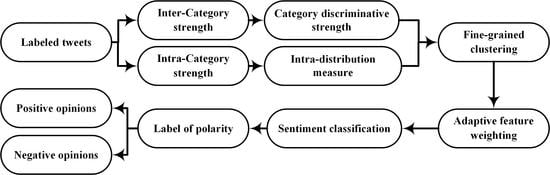
The machine learning-based approach employs a supervised learning technique to train a text classifier using a manually labeled training dataset and extract the features. More specifically, the process can be described as follows. Given a training dataset consisting of labeled text documents, D = {(d1, l1), …, (dm, lm)}, where di represents a document belonging to the initial training corpus, D, and li is the manual label reflecting a specific preset class among the set of classes, L. Here, the main task is to detect unlabeled text data by generating an effective classification model from the labeled training dataset [19]. Figure 1 depicts the structure of Twitter sentiment analysis based on the machine learning approach. Various formats of sources such as blogs, reviews, etc., are utilized as input data for Twitter sentiment analysis. Here, useful features are selected by a feature extractor for subsequent processing, which is critical to sentiment analysis. This is because the combination of different features plays a crucial role in the classification. The classifier is then trained by a machine learning algorithm to evaluate the degree of polarity and assign a corresponding label to the tested instance [25,26,27].
Various learning algorithms have been adopted for the machine learning-based approach, including Support Vector Machine (SVM), Decision Tree (DT), Naïve-Bayes (NB), and NN, etc. SVM has been proved to be a powerful classification algorithm, especially in processing a massive number of features [28,29,30]. However, the weakness of low interpretability and computational overhead limits its usage. DT is another popular algorithm where the features and corresponding classes are reflected in the form of tree structure. It is well understood, and can be easily employed to classify textual data. However, exploring the features is restricted owing to its rigid tree structure, and feature overfitting may degrade the performance [31,32,33]. NB is a commonly used method for sentiment analysis due to its advantages of effectiveness and simplicity. It is used to select the category of the highest probability for the unlabeled text based on the probability theory [19,34,35,36].
The NN classifier employs a network structure that is composed of a group of connected units, where each input represents a term and an output is generated from a function to represent the corresponding category. The dependence relations are represented by weighted edges between the units. Assume that a tested document_d is evaluated by the NN classifier. The term weight, w, is viewed as an input to the units, and the output of the units is the decision of the category that is obtained by activating the units of the network [37]. Perceptron is a simple linear NN classifier, which is also called a single-layer perceptron, which applies the Heaviside step function to activate the units of the network [38]. Another type of linear NN classifier incorporating logistic regression achieves good classification performance [39]. Here a non-linear NN classifier is implemented by constructing one or more layers of units. In [40] a non-linear NN was applied to the task of topic spotting, which models higher-order interaction between the terms. Due to the advantage of the NN classifier in processing data with multiple attributes, recently, many researches have been focusing on the study of the NN technique. A novel NN model (ConvGRNN and LSTM-GRNN) was proposed to evaluate the document-level sentiment analysis, where the semantics of sentences and corresponding correlations are encoded by the document representation [41]. In [42] a Mixed Neural Network (MNN) was introduced to solve the classification problem, which combines a rectifier Neural Network and Long Short-Term Memory (LSTM). A neural architecture and two extensions of Long Short-Term Memory (LSTM) [43] were presented to handle the task of targeted aspect-based sentiment analysis.
2.4. Feature Weighting
Feature weighting is a process of assigning appropriate weight to individual features in accordance with their relevance to the given domains. It is generally thought of as the generalization of feature selection, where the presence of a feature serves as the criterion for its extraction [44]. Each feature is represented as a binary vector, wherein “0” denotes the absence of the feature (evict the feature), and “1” denotes the presence (keep the feature) [19]. A variety of feature weighting methods have been introduced, and DF is the simplest one, where the “single appearance” of a word is equivalent with “multiple appearances” [45]. It counts the number of documents in which a word occurs, and uses the value to represent the corresponding document. TF is another criterion that explores feature weighting in a different direction. It is based on the intuition that the term of multiple appearances is more important than that of a single appearance [46]. Here, the frequency of a word occurring in a document is counted, which is used to represent the document, and is expressed as:
Here, tfi,j represents the frequency of word_i in document_j, and N is the number of documents in category_ck. TF has been proved to be effective, but its performance is degraded with the multi-domain dataset because of the simple measure of words. Term Frequency and Inverse Document Frequency (TF-IDF) is a “state-of-the-art” method of feature weighting [47], which comprehensively measures the appearance frequency and distribution of words in assigning the weights, and it is obtained as:
where idf(i,D) measures how much information word_i provides to represent document_j in document set_D, which is formulated as:
Here, |{i∈D:i∈j}| represents the number of documents containing word_i in D. The TF-IDF is effective in selecting important words in a document while eliminating common words, yielding good performance in terms of classification accuracy. Part of Speech-based Weighting (PSW) is another novel feature weighting approach improving the accuracy of Twitter sentiment analysis. It clusters unique words of the categories into different subsets based on the word’s Part Of Speech (POS) feature, which is shown in Table 1.
The words in the subsets are weighted considering the intra-category relevance of the words, which is measured as:
Here, wfi,j represents the assigned weight for word_i in subset_j, and x is the weight of the value of 2, 1.5, or 1 for each of the three subsets, which is given to leverage the role of the words in different subsets in affecting the orientation of the sentiment. E[Fj] refers to the expected frequency of the words in subset_j which is computed as:
Note from Equation (4) that only when the TF value of a word is larger than the expected frequency of the subset, the weight is adjusted. This indicates that the word is more informative than the average level of the subset. The PSW method incorporates a clustering technique to classify the words and assign weights based on the semantical meaning and hierarchical relevance of the words, allowing effective feature weighting.
3. The Proposed Scheme
In this section a novel adaptive feature weighting scheme is proposed called CDS-C (Category Discriminative Strength with Chi-square model), which properly measures the inter-category and intra-category significance of a feature. A new mathematical model called Category Discriminative Strength (CDS) is presented to measure the inter-category discriminative strength of the features, while a modified Chi-square model is introduced to measure the dependency of the features in intra-category. Also, a fine-grained clustering strategy is proposed to precisely define the margin of discriminative features and aggregate the features of similar distributions for efficient feature weighting. Furthermore, an adaptive weighting strategy is proposed to properly decide the weight for each feature.
3.1. Motivation
The main objective of the feature weighting of sentiment analysis is to assign an appropriate weight for every single word in order to reflect its relative significance in the feature space, which in turn allows accurate prediction of the sentiment. Generally, many supervised feature weighting approaches assume that the inter-category distribution of a feature plays a major role in feature weighting, while ignoring its intra-category distribution. Nevertheless, the researchers have been questioning feature weighting based on only the inter-category distribution of the features. It has been proved that incorporating the two distributions is superior to using only one with respect to the measurement of the significance of the feature, and as a result yields a better classification performance. The inter-category and intra-category distribution of the features are equally important in feature weighting.
Intuitively, for a specific word, the more evenly a word is distributed in the feature space, the weaker it distinguishes the category. For example, even though conjunction words widely appear in a document, they hardly represent any category. It is generally believed that the words of large CDS mostly occur in only one or a few categories. Note that adjective words more likely appear in the given category to express the sentiment. Therefore, it is highly likely that the words of non-uniform distribution in the entire categories represent a specific category, and thus a larger weight needs to be assigned. While inter-category distribution is important to characterize the significance of a word in the decision of the weight, intra-category distribution of the word is also crucial in measuring its significance. Specifically, the distribution of a word within a certain category reflects its dependency on that category. More accurate weight could be obtained by incorporating the dependency. Thus, in the proposed scheme, CDS is used to measure the inter-category distribution of the word, while the property of intra-category distribution is formulated using the Intra-Distribution Measure (IDM). The feature weight is then finally computed based on the two measures.
3.2. Category Discriminative Strength
In order to characterize the inter-category distribution, a specific VSM is constructed to represent the feature weight of the words among the whole categories. Here, every single category, ci (C, C = {c1, …, cn}, n ≥ 1) is viewed as a vector on the feature space, and it is represented as . n is the number of the categories, and denotes the feature value of word_w based on target category_ci. In TF the number of occurrences of a word for a certain document is counted to represent the feature weight of the document. Typically, the greatest feature value among the whole categories is utilized as the global feature weight of the word for that category, which is denoted as:
This approach effectively analyzes the relative weight of the words based on the frequency. However, the discriminative strength of the words is not properly considered. Note that appropriately reflecting the discriminative strength of the word is crucial for the measure of inter-category distribution. Therefore, the frequency with which a word appears in all of the whole documents of a category, cf, is employed instead of TF, and then the VSM is expressed as:
Assume that word_w occurs only in category_c1. Then, the VSM becomes one element vector, which indicates that word_w is solely relevant to class_c1. Note that the more categories a word belongs to, the less discriminative information the word retains to distinguish a certain category. Especially, when , word_w is distributed uniformly in the class space, which indicates that word_w is meaningless in representing any category.
In order to effectively measure the inter-class distribution, a novel model called CDS is introduced to measure how much discriminative information a word contains in representing a category, which is expressed as:
Here, n is the number of categories containing word_wμ in the training dataset, and cfwμ,cν is the frequency of word_wμ appearing in category_cν, which is obtained by summing up the total number of occurrences of word_wμ appearing within all the documents of that category. CDS(wμ,cν) denotes the total frequency distance of word_wμ on the pre-measured category_cν in the feature space. If CDS(wμ,cν) > 0, word_wμ is viewed as having positive relevance to category_cν, and owns discriminative information with respect to that category. Otherwise, it is regarded as meaningless.
Assume that word_wμ appears in n categories. Then, a queue Qp is built with the sorted values of CDS with respect to n individual categories in descending order, which is expressed as Qp = CDS(wμ,cα) ≥ … ≥ CDS(wμ,cj) (1 ≤ α ≤ m, 1 ≤ j ≤ n). Here, CDS(wμ,cα) represents the highest CDS value of the n elements, which indicates that category_cα is the choice for word_wμ. The degree of choice for word_wμ considering multiple categories is formulated as:
Here, word_wμ is supposed to appear in category_cj(1 ≤ j ≤ m), and Dinter(wμ,cν) represents the degree of choice of category_cν for word_wμ measuring how much contribution word_wμ makes for category_cν in predicting the polarity of the tested document. Using only one category for a word may not be enough because every presence of the word in other categories is also meaningful. Therefore, the intra-category measure of the words in one category also needs to be analyzed in order to precisely characterize the words.
Similar to Qp, another queue, Qq = CDS(wα,cν) ≥ … ≥ CDS(wi,cν), is built with the sorted values of CDS(wi,cν) of word_wi (1 ≤ i ≤ m) belonging to category_cν in descending order. The degree of intra-category significance of a word is then measured as:
With word_wi (1 ≤ i ≤ m) in category_cν, Dintra(wμ,cν) measures the intra-category significance of word_wμ. Incorporating Dinter(wμ,cν) and Dintra(wμ,cν), the discriminability of word_wμ for category_cν is measured as:
Based on the relative frequency and discriminability, word_wμ is represented as a vector, DisVector, as depicted in Figure 2. Here, the word is located at the origin, and the pointer that originated from it represents the position of the discriminability of the word.
Obviously, Lengthi and θi are needed to be computed for constructing DisVector for a word. The relative frequency, cf(wμ,cν), and discriminability, Φ(wμ,cν), are utilized for obtaining them as:
Here, λ is a linear factor that maps the range of Φ(wx,cy), [Φmin, Φmax], into [0,π/2]. The value of Φmin and Φmax are computed based on the training dataset. Refer to Figure 2. The degree of discriminability of word_i, Di, is obtained as:
The discriminability of a word is characterized by DisVector in terms of the orientation of the discriminability and strength of the word.
3.3. Intra-Distribution Measure (IDM)
The intra-distribution of a word is important in reflecting its dependency on a category. Inverse Document Frequency (IDF) is commonly adopted, which measures how much information a word offers in representing the category. It measures the degree of occurrence of a word across all the documents, and is expressed as:
Here, N is the number of documents in the training dataset, and |{d ∈ D: w ∈ d}| denotes the number of documents containing word_w. IDF has been incorporated into various schemes including TF-IDF to decrease the weight of frequently appearing words and increase the weight of rare words. This is a coarse-grained approach because it supposes that rare words are more important than common ones. In this paper a fine-grained Intra-Distribution Measure called IDM is introduced to analyze the words, which incorporates the dependency derived from Chi-square statistics and the occurrence of words in the document. It is expressed as:
Here, χ2(wi,cj) is the Chi-square value measuring the dependency of word_wi on category_cj. It is denoted as:
Table 2 lists the cases of the sums of the frequencies of the words. Here, . , and . m is the number of documents word_wi appears in category_cj, and n is the number of categories except class_cj. M denotes the sum of cf value of all the words in category_cj, and N is computed by summing the value of cf of words of categories except class_cj. Note that, unlike the conventional Chi-square method, is employed as the input of the Chi-square calculation to avoid the weakness of incorrectly overestimating the role of low-frequency words. The proposed IDM is based on the intuition that the words of high document frequency are relatively more important. By incorporating the dependency of the words on the category, more accurate measurement of the intra-distribution significance of the words is obtained.
3.4. Feature Clustering and Weighting
In order to efficiently analyze a large amount of features extracted from the training dataset, a feature clustering and weighting strategy is proposed. The clustering is performed to partition the features into representative groups generating a smaller classification model and allow a higher accuracy of sentiment prediction. In this paper two representative groups, GD and GN, are constructed to accommodate the distinctive and non-distinctive terms of a category [48].
Instinctively, an emotive word is representative and possesses enough distinctive information reflecting the sentiment orientation of a document. In order to accurately extract emotive words, firstly, all the documents belonging to a category are parsed through the Part of Speech (POS) tagger, and a POS tag is assigned to each word.
The unique terms with the tag of Verb, Adjective, or Adverb are regarded as emotive indicators to be clustered into GD, and the words with other tags are put in GN. However, as some words may co-occur in multiple categories, not all of the emotive words in a category are distinctive for that category. Since the words in the same cluster are expected to display similar inter-category distributions, the distribution of the target word over the whole feature space is examined. Then, the words of similar distribution are clustered [49]. The relative distance of similarity, Di,j, between word_wi and cluster_Gθ (θ = D ∨ N) is obtained as:
Here the distance is measured by the Euclidean norm of the Φ value of word_wi for category_cj from the expectation. Recall that the Φ value measures the discriminability of a word for the given category. Therefore, it is utilized in measuring the status of the word in that category. exp(Gθ,cj) is the expectation of word_wi for category_cj, and it is computed as:
Here p is the number of unique words in cluster_Gθ. The average distance, Dθ (θ = D ∨ N), of the words from cluster_Gθ is obtained as:
Then, all the words of cluster_GD are compared with the average distance, DD, to extract the relevant emotive words. If DD ≥ Di,j, word_wi is not regarded as relevant to GD. Otherwise, it is put to GN. Note that cluster_GD accommodates highly relevant words of large discriminative information. Then, the weight for word_wi, W, is calculated, reflecting its significance in terms of inter-class and intra-class distribution, and it is expressed as:
Here, the weight assigned to word_wi of cluster_GD and cluster_GN of class_ck are represented as W(wi,GD,ck) and W(wi,GN,ck), respectively, and p and q are the number of unique words of GD and GN, respectively. Note that cluster_GD retains emotive words obtained with fine-grained selection, and reflects the ratio of inter-distribution measures between GD and GN, capturing the intuition that the emotive words greatly represent the orientation of sentiment of the document. IDM(wi,ck) is employed as an intra-category distribution metric to accurately reflect the degree of the significance of word_wi in class_ck.
3.5. Sentiment Estimation
Bayesian theorem, as a supervised learning technique, is commonly applied to the sentiment analysis. In this paper the Multinomial Naïve-Bayes (MNB) is employed as the classifier to predict the polarity of the tested documents. Assuming that tested document_d is represented as a vector <w1, …, w|W|>, the MNB estimates the label of the Maximum A Posteriori (MAP) category and the probability of the category membership of d for category_c using Equations (23) and (24) [50]:
Here W is the number of unique words in document_d, wi represents the i-th word of d, and C is the set of all the possible labels. P(wi|c) is the conditional probability of word_wi (1 ≤ i≤ |W|) belonging to document_d with the category label_c. Observe from Equation (24) that multiplying |W| conditional probabilities may cause floating point underflow, which results in incorrectly predicting the sentiment. Hence, the addition of the logarithms of the probabilities is used instead of the multiplication of the probabilities as follows.
The prior probability, P(c), is computed as:
Here Nc is the number of documents in category_c, and N is the entire number of documents in the training data. Note that incorporating the feature weights into both the classification formula and conditional probability model improves the performance of the classifier of Naïve-Bayes [51]. Therefore, the conditional probability in Equation (25) is modified as:
Here W(wi,Gθ,c) is the importance degree of word in terms of inter-class and intra-class distribution, and it is computed based on Equations (21) and (22). λ(cj,c) is a binary function judging whether the two input parameters are equal or not. It is defined as:
As the feature weights are incorporated into the MNB model for calculating the probability of the target document belonging to category_c, the class label with the highest probability is selected as the most suitable one for that document. Note that the synonyms are separately assigned the feature weight to reflect its significance, causing a respective effect in sentiment analysis.
4. Performance Evaluation
In order to demonstrate the effectiveness of the proposed feature weighting scheme for Twitter sentiment analysis, extensive experiments are carried out. Also, the results are compared with the existing schemes such as DF, TF, TF-IDF, and PSW.
4.1. Experiment Setting
The proposed CDS-C scheme is evaluated using Matlab, which consists of three components including the preprocessor, POS tagging API, and Bayes-based text classifier. The preprocessor is performed to remove stop-words and punctuations, and normalize the training dataset into a customized form, which makes it accessible by a POS tagger and features extractor. A Matlab-based function is utilized to implement the Stanford POS tagger [52,53], which offers the API that is used to obtain the POS tag for each word in the training dataset. The Bayes-based text classifier is implemented to apply the Baye’s theorem in the analysis of the orientation of the sentiment and prediction of the polarity (positive/negative) of the tested document. In this paper the MNB classifier is utilized as the text classifier with the assumption of feature independence. The workload in the experiments is extracted from Sentiment 140, which is a benchmark dataset derived from Twitter API, and widely adopted in the sentiment analysis [54]. The workload is composed of 1,600,000 documents of labeled tweets where one half is labeled as positive and the other is labeled as negative. The data of Sentiment 140 covers a wide range of domains and data characteristics [55], and two instances are shown in Figure 3. Each data consists of six attributes: the polarity indicator (0 = negative, 4 = positive), user id, posting time, query condition, username, and text of the tweet. Four metrics are adopted to evaluate the performance of feature weighting in sentiment analysis: accuracy, precision, recall, and F1-score [19].
4.2. Experimental Results
Three groups of cross-validated experiments are carried out to compare the proposed scheme with the existing ones. As a workload of Sentiment 140 is built from 800,000 negative and 800,000 positive documents of labeled tweets, the data is reconstructed as pairs of one negative and one positive tweet. For each experiment, 10,000 distinct random numbers (half odd and half even) are generated using the MATLAB function, ranging from one to 1,600,000. A training dataset is then constructed by extracting the tweets of the corresponding index from Sentiment 140, which is composed of 5000 negative and 5000 positive randomly selected documents. The tested dataset is selected from the remaining 1,500,000 documents of tweets.
The first group of experiments tries to investigate the performances in processing the tested data with balanced class distribution. Here, the tested datasets ranging from 500 to 6000 elements are built, consisting of equal number of positive and negative randomly selected documents. Secondly, two experiments are implemented to compare the performances of the schemes in handling biased tested data, consisting of solely positive or negative instances. Finally, they are evaluated with the tested documents of random polarity.
Figure 4 shows the performance of classification of the five schemes when the size of the balanced tested dataset varies from 500 to 6000. Observe from the figures that the proposed CDS-C scheme consistently outperforms the other schemes for all four metrics regardless of the size of the tested data. Evaluating the tweets that have negative and positive polarity of the same size is common. The proposed scheme presents the highest accuracy, precision, recall, and F1-score, which indicates that it is very sensitive to the orientation of sentiment, and is able to classify the tested data into the correct category. This is achieved by the weights that were computed in accordance with both inter-category and intra-category feature relevance, and the discriminative features. Moreover, the proposed models of CDS and IDM properly measure the discriminability of the features of the training dataset, which contributes to quantify the usefulness of the features. In general, the classification performance tends to degrade when the number of the tested data increases. This is because a training corpus of limited size cannot sufficiently cover the increased size of the tested data. As depicted in Figure 4a, the accuracy slightly decreases as the number of tested documents increases from 500 to 6000. Also, it can be seen from Figure 4a,d that the accuracy and F1-score of the DF are superior than TF because considering either the presence or absence of features allows higher classification performance than considering only their frequencies [56].
Table 3 shows two tweets extracted from Sentiment 140, and Table 4 shows a comparison of the polarity label assigned with the five approaches evaluating the tested tweets of Table 3. Observe from Table 3 that the indicator is the predefined polarity label as “0” for negative and “4” for positive. As Table 4 shows, P(neg|test) and P(pos|test) are the final sentiment values generated by the MNB classifier of the tested tweets in the negative and positive categories, respectively. The final polarity label is obtained by comparing the two values.
Figure 5 presents the performance of the five schemes in terms of the accuracy with the balanced training dataset, but biased tested data. As observed from Figure 5a,b, the proposed approach always produces the highest accuracy compared to the other four schemes regardless of the polarity of the tested documents. It is challenging to analyze biased tweets using a training dataset of a limited size. Since a specific training dataset has an inclination on the tested instances of a certain polarity, a classifier trained using it may not be robust enough. Note that the proposed fine-grained clustering strategy accurately defines the boundary of the features, and groups the features into different clusters. Also, the discriminative features are effectively aggregated considering its significance and distribution. As a result, the proposed scheme can allow high classification accuracy in processing biased tested data. Observe from Figure 5a that the DF scheme achieves the second-highest accuracy, while TF shows the lowest accuracy. However, they display opposite performances for the document of negative polarity as shown in Figure 5b. This is because DF and TF weight the features based on the absence and frequency, respectively. Thus, the schemes are suitable for specific tested data, while their performances are significantly affected by the polarity of the tested data.
In order to validate the robustness and efficiency of the schemes, the experiments are conducted with the tested dataset formed with the documents of random polarity. This set of experiments is complementary to the second group in evaluating biased tested tweets. Observe from Figure 6 that the proposed scheme consistently shows the highest performance in terms of all the four metrics. An unreasonable assignment of the weight to the features causes inaccurate decision of the polarity. Since the proposed adaptive weighting strategy computes the weight considering the inter-category and intra-category relevance, dependency, and distribution of the features, it can exhibit robust performance. This confirms that the proposed scheme is effective regardless of the dataset with respect to the size and polarity of the tested dataset.
5. Conclusions
In this paper a novel feature weighting scheme has been presented for the sentiment analysis of tweet data. It comprehensively measures the significance of the features in both inter-category and intra-category distribution, and an analytical model characterizing the discriminability of the feature was introduced to precisely measure how much discriminative information a feature possesses. Also, a modified Chi-square statistics model was proposed to measure the relative relevance of a feature with the corresponding category. A new fine-grained clustering strategy was adopted to properly group the features of similar inter-category distribution, which allows accurate text classification. Extensive experiments were conducted using benchmark workloads, which demonstrate that the proposed scheme is consistently superior to the existing approaches in terms of four metrics including accuracy.
Since the proposed scheme is based on the dependence of each feature to the corresponding category, the length of the sentence does not directly affect the performance of the proposed method. A more precise model on the relation between the measures will be investigated in the future. As each word has a different feature weight reflecting its importance degree for different categories, the polarity of a sentence having two different opinions is determined by the weights obtained using the MNB text classifier. A new approach including the NN technique will also be developed for handling different or opposite opinions. In the proposed scheme the emoticons are detected and removed using the MATLAB function of the tokenized document. Since emotions usually contain some sentiments of people, a methodology effectively dealing with them will be included in future work.
The proposed scheme is currently performed in the MATLAB environment, manually evaluating the labeled tweets. Its performance will be tested by processing real-time information of the Twitter platform via the Twitter API, and more advanced text preprocessing techniques will be incorporated to improve the quality of classification of the sentiment. Further enhancements include the portability to other platforms such as mobile devices and the incorporation of Latent Dirichlet Allocation (LDA) technique to automatically identify the number of attributes of corpus [57,58,59,60].
Author Contributions
Conceptualization, Y.W. and H.Y.Y.; Methodology, Y.W.; Software, Y.W.; Validation, Y.W. and H.Y.Y.; Formal Analysis, Y.W.; Investigation, Y.W. and H.Y.Y.; Resources, Y.W.; Data Curation, Y.W.; Writing—Original Draft Preparation, Y.W.; Writing—Review & Editing, Y.W. and H.Y.Y.; Visualization, Y.W.; Supervision, H.Y.Y.; Project Administration, H.Y.Y.; Funding Acquisition, H.Y.Y.
Funding
This research was supported by Institute for Information & communications Technology Promotion(IITP) grant funded by the Korea government(MSIT) (No.2016-0-00133, Research on Edge computing via collective intelligence of hyperconnection IoT nodes), Korea, under the National Program for Excellence in SW supervised by the IITP(Institute for Information & communications Technology Promotion)(2015-0-00914), Basic Science Research Program through the National Research Foundation of Korea (NRF) funded by the Ministry of Education, Science and Technology (2016R1A6A3A11931385, Research of key technologies based on software defined wireless sensor network for realtime public safety service, 2017R1A2B2009095, Research on SDN-based WSN Supporting Real-time Stream Data Processing and Multiconnectivity), the second Brain Korea 21 PLUS project.
Acknowledgments
The authors are grateful to the supports from the Sungkyunkwan University for sample collection.
Conflicts of Interest
The authors declare no conflict of interests.
References
- Deng, Z.H.; Tang, S.W.; Yang, D.Q.; Ming, Z.; Li, L.Y.; Xie, K.Q. A comparative study on features weight in text categorization. In Proceedings of the Asia-Pacific Web Conference, Berlin, Germany, 4 April 2004. [Google Scholar]
- Deng, Z.H.; Luo, K.H.; Yu, H.L. A study of supervised term weighting scheme for sentiment analysis. Expert Syst. Appl. 2014, 41, 3506–3513. [Google Scholar] [CrossRef]
- Xia, Z.; Lv, R.; Zhu, Y.; Ji, P.; Sun, H.; Shi, Y.Q. Fingerprint liveness detection using gradient-based texture features. Signal Image Video Process. 2017, 11, 381–388. [Google Scholar] [CrossRef]
- Salima, B.; Barigou, F.; Belalem, G. Sentiment analysis at document level. In Proceedings of the International Conference on Smart Trends for Information Technology and Computer Communications, Singapore, 6 August 2016. [Google Scholar]
- Parlar, T.; Özel, S.A.; Song, F. QER: A new feature selection method for sentiment analysis. Int. J. Mach. Learn. Cybern. 2018, 8, 10. [Google Scholar] [CrossRef]
- Zhou, H.; Guo, J.; Wang, Y.; Zhao, M. A feature selection approach based on interclass and intraclass relative contributions of terms. Comput. Intell. Neurosci. 2016, 2016, 8. [Google Scholar] [CrossRef] [PubMed]
- Zheng, L.; Wang, H.; Gao, S. Sentimental feature selection for sentiment analysis of Chinese online reviews. Int. J. Mach. Learn. Cybern. 2018, 9, 75–84. [Google Scholar] [CrossRef]
- Debole, F.; Sebastiani, F. Supervised term weighting for automated text categorization. In Proceedings of the Text Mining and Its Applications, 1st ed.; Janusz, K., Ed.; Springer: Berlin, Germany, 2004; Volume 138, pp. 81–97. [Google Scholar]
- Chen, K.; Zhang, Z.; Long, J.; Zhang, H. Turning from TF-IDF to TF-IGM for term weighting in text classification. Expert Syst. Appl. 2016, 66, 245–260. [Google Scholar] [CrossRef]
- Wang, Y.; Sun, L.; Wang, J.; Zheng, Y.; Youn, H.Y. A Novel Feature-Based Text Classification Improving the Accuracy of Twitter Sentiment Analysis. In Proceedings of the Advances in Computer Science and Ubiquitous Computing, Singapore, 18 December 2017. [Google Scholar]
- Yang, A.; Jun, Z.; Lei, P.; Yang, X. Enhanced twitter sentiment analysis by using feature selection and combination. In Proceedings of the Security and Privacy in Social Networks and Big Data, Hangzhou, China, 16–18 November 2015. [Google Scholar]
- Jose, A.K.; Bhatia, N.; Krishna, S. Twitter Sentiment Analysis; Seminar Report; National Institute of Technology Calicut: Kerala, India, 2010. [Google Scholar]
- Krouska, A.; Troussas, C.; Virvou, M. The effect of preprocessing techniques on Twitter Sentiment Analysis. In Proceedings of the International Conference on Information, Intelligence, Systems & Applications, Chalkidiki, Greece, 13–15 July 2016. [Google Scholar]
- Wikipedia Sentiment Analysis. Available online: https://en.wikipedia.org/wiki/Sentiment_ analysis (accessed on 12 November 2018).
- Pang, B.; Lee, L. Opinion Mining and Sentiment Analysis, 1st ed.; Now Publishers Inc.: Boston, MA, USA, 2008; pp. 1–135. [Google Scholar]
- Mingqing, H.; Bin, L. Mining and summarizing customer reviews. In Proceedings of the Tenth ACM SIGKDD International Conference on Knowledge Discovery and Data Mining, Washington, DC, USA, 22–25 August 2004. [Google Scholar]
- Nielsen, F.A. A new ANEW: Evaluation of a word list for sentiment analysis in microblogs. arXiv, 2011; arXiv:1103.2903. [Google Scholar]
- Mohammad, S.M.; Kiritchenko, S.; Zhu, X. NRC-Canada Building the state-of-the-art in sentiment analysis of tweets. arXiv, 2013; arXiv:1308.6242. [Google Scholar]
- Kolchyna, O.; Souza, T.T.; Treleaven, P.; Aste, T. Twitter sentiment analysis: Lexicon method, machine learning method and their combination. arXiv, 2015; arXiv:1507.00955. [Google Scholar]
- Hailong, Z.; Wenyan, G.; Bo, J. Machine Learning and Lexicon Based Methods for Sentiment Classification: A Survey. In Proceedings of the Web Information System and Application Conference, Tianjin, China, 12–14 September 2014. [Google Scholar]
- De Diego, I.M.; Fernández-Isabel, A.; Ortega, F.; Moguerza, J.M. A visual framework for dynamic emotional web analysis. Knowl.-Based Syst. 2018, 145, 264–273. [Google Scholar] [CrossRef]
- Cambria, E. Affective computing and sentiment analysis. IEEE Intell. Syst. 2016, 31, 102–107. [Google Scholar] [CrossRef]
- Machado, M.T.; Pardo, T.A.; Ruiz, E.E.S. Creating a Portuguese context sensitive lexicon for sentiment analysis. In Proceedings of the International Conference on Computational Processing of the Portuguese Language, Cham, Switzerland, 24 September 2018. [Google Scholar]
- Al-Moslmi, T.; Albared, M.; Al-Shabi, A.; Omar, N.; Abdullah, S. Arabic senti-lexicon: Constructing publicly available language resources for Arabic sentiment analysis. J. Inf. Sci. 2018, 44, 345–362. [Google Scholar] [CrossRef]
- Feldman, R. Techniques and applications for sentiment analysis. Commun. ACM 2013, 56, 82–89. [Google Scholar] [CrossRef]
- Giachanou, A.; Crestani, F. Like it or not: A survey of Twitter sentiment analysis methods. ACM Comput. Surv. 2016, 49, 28. [Google Scholar] [CrossRef]
- Fernández-Isabel, A.; Prieto, J.C.; Ortega, F.; de Diego, I.M.; Moguerza, J.M.; Mena, J.; Galindo, S.; Napalkova, L. A unified knowledge compiler to provide support the scientific community. Knowl.-Based Syst. 2018, 161, 157–171. [Google Scholar]
- Jaramillo, F.; Orchard, M.; Muñoz, C.; Antileo, C.; Sáez, D.; Espinoza, P. On-line estimation of the aerobic phase length for partial nitrification processes in SBR based on features extraction and SVM classification. Chem. Eng. J. 2018, 331, 114–123. [Google Scholar] [CrossRef]
- López, J.; Maldonado, S.; Carrasco, M. Double regularization methods for robust feature selection and SVM classification via DC programming. Inf. Sci. 2018, 429, 377–389. [Google Scholar] [CrossRef]
- Maldonado, S.; López, J. Dealing with high-dimensional class-imbalanced datasets: Embedded feature selection for SVM classification. Appl. Soft. Comput. 2018, 67, 94–105. [Google Scholar] [CrossRef]
- Achlerkar, P.D.; Samantaray, S.R.; Manikandan, M.S. Variational mode decomposition and decision tree based detection and classification of power quality disturbances in grid-connected distributed generation system. IEEE Trans. Smart Grid 2018, 9, 3122–3132. [Google Scholar] [CrossRef]
- Liu, X.; Li, Q.; Li, T.; Chen, D. Differentially private classification with decision tree ensemble. Appl. Soft. Comput. 2018, 62, 807–816. [Google Scholar] [CrossRef]
- Li, F.; Zhang, X.; Zhang, X.; Du, C.; Xu, Y.; Tian, Y.C. Cost-sensitive and hybrid-attribute measure multi-decision tree over imbalanced data sets. Inf. Sci. 2018, 422, 242–256. [Google Scholar] [CrossRef]
- Li, T.; Li, J.; Liu, Z.; Li, P.; Jia, C. Differentially private naive bayes learning over multiple data sources. Inf. Sci. 2018, 444, 89–104. [Google Scholar] [CrossRef]
- Lee, C.H. An information-theoretic filter approach for value weighted classification learning in naive Bayes. Data Knowl. Eng. 2018, 113, 116–128. [Google Scholar] [CrossRef]
- Xu, S. Bayesian Naïve Bayes classifiers to text classification. J. Inf. Sci. 2018, 44, 48–59. [Google Scholar] [CrossRef]
- Sebastiani, F. Machine learning in automated text categorization. ACM Comput. Surv. 2002, 34, 1–47. [Google Scholar] [CrossRef] [Green Version]
- Ng, H.T.; Goh, W.B.; Low, K.L. Feature selection, perceptron learning, and a usability case study for text categorization. In Proceedings of the 20th Annual International ACM SIGIR Conference on Research and Development in Information Retrieval, Philadelphia, PA, USA, 27–31 July 1997. [Google Scholar]
- Schütze, H.; Hull, D.A.; Pedersen, J.O. A comparison of classifiers and document representations for the routing problem. In Proceedings of the 18th Annual International ACM SIGIR Conference on Research and Development in Information Retrieval, Seattle, WA, USA, 9–13 July 1995. [Google Scholar]
- Wiener, E.; Pedersen, J.O.; Weigend, A.S. A neural network approach to topic spotting. In Proceedings of the 4th Annual Symposium on Document Analysis and Information Retrieval (SDAIR-95), Las Vegas, NV, USA, 24–26 April 1995. [Google Scholar]
- Tang, D.; Qin, B.; Liu, T. Document modeling with gated recurrent neural network for sentiment classification. In Proceedings of the Conference on Empirical Methods in Natural Language Processing, Lisbon, Portugal, 17–21 September 2015. [Google Scholar]
- Dong, H.; Supratak, A.; Pan, W.; Wu, C.; Matthews, P.M.; Guo, Y. Mixed neural network approach for temporal sleep stage classification. IEEE Trans. Neural Syst. Rehabil. Eng. 2018, 26, 324–333. [Google Scholar] [CrossRef]
- Ma, Y.; Peng, H.; Khan, T.; Cambria, E.; Hussain, A. Sentic LSTM: A Hybrid Network for Targeted Aspect-Based Sentiment Analysis. Cogn. Comput. 2018, 10, 639–650. [Google Scholar] [CrossRef]
- Xia, Z.; Shi, T.; Xiong, N.N.; Sun, X.; Jeon, B. A Privacy-Preserving Handwritten Signature Verification Method Using Combinational Features and Secure KNN. IEEE Access 2018, 6, 46695–46705. [Google Scholar] [CrossRef]
- Zheng, Y.; Jeon, B.; Sun, L.; Zhang, J.; Zhang, H. Student’s t-hidden Markov model for unsupervised learning using localized feature selection. IEEE Trans. Circuits Syst. Video Technol. 2018, 28, 2586–2598. [Google Scholar] [CrossRef]
- Yan, X.; Chen, L. Term-frequency based feature selection methods for text categorization. In Proceedings of the International Conference on Genetic and Evolutionary Computing, Shenzhen, China, 13–15 December 2010. [Google Scholar]
- Xia, Z.; Wang, X.; Sun, X.; Wang, Q. A secure and dynamic multi-keyword ranked search scheme over encrypted cloud data. IEEE Trans. Parallel Distrib. Syst. 2015, 27, 340–352. [Google Scholar] [CrossRef]
- Wang, Y.; Kim, K.; Lee, B.; Youn, H.Y. Word clustering based on POS feature for efficient twitter sentiment analysis. Hum.-Centric Comput. Inf. Sci. 2018, 8, 17. [Google Scholar] [CrossRef]
- Baker, L.D.; McCallum, A.K. Distributional clustering of words for text classification. In Proceedings of the 21st Annual International ACM SIGIR Conference on Research and Development in Information Retrieval, Melbourne, Australia, 24–28 August 1998. [Google Scholar]
- Stanford Naïve Bayes Text Classification. Available online: http://nlp.stanford.edu/IR-book /html/htmledition/naive-bayes-text-classification-1.html (accessed on 13 November 2018).
- Zhang, L.; Jiang, L.; Li, C.; Kong, G. Two feature weighting approaches for naive bayes text classifiers. Knowl.-Based Syst. 2016, 100, 137–144. [Google Scholar] [CrossRef]
- Stanford Log-Linear Part-of-Speech Tagger. Available online: http://nlp.stanford.edu/softw are/tagger.shtml (accessed on 5 October 2018).
- Matlab-Stanford-Postagger. Available online: https://github.com/musically-ut/matlab-stanf ord-postaggr (accessed on 3 May 2018).
- Sentiment 140. Available online: http://help.sentiment140.com/home (accessed on 6 May 2018).
- Liangxiao, J.; Dianhong, W.; Zhihua, C. Discriminatively weighted naïve bayes and its application in text classification. Int. J. Artif. Intell. Tools 2012, 21, 1250007. [Google Scholar]
- Pang, B.; Lee, L.; Vaithyanathan, S. Thumbs up?: Sentiment classification using machine learning techniques. In Proceedings of the ACL–02 Conference on Empirical Methods in Natural Language Processing, Philadelphia, PA, USA, 6–7 July 2012. [Google Scholar]
- Zhong, Y.; Huang, R.; Zhao, J.; Zhao, B.; Liu, T. Aurora image classification based on multi-feature latent dirichlet allocation. Remote Sens. 2018, 10, 233. [Google Scholar] [CrossRef]
- Li, H.; Yang, X.; Jian, L.; Liu, K.; Yuan, Y.; Wu, W. A sparse representation-based image resolution improvement method by processing multiple dictionary pairs with latent Dirichlet allocation model for street view images. Sustain. Cities Soc. 2018, 38, 55–69. [Google Scholar] [CrossRef]
- Schwarz, C. Ldagibbs: A command for topic modeling in Stata using latent Dirichlet allocation. Stata J. 2018, 18, 101–117. [Google Scholar] [CrossRef]
- Joo, S.; Choi, I.; Choi, N. Topic Analysis of the Research Domain in Knowledge Organization: A Latent Dirichlet Allocation Approach. Knowl. Organ. 2018, 45, 170–183. [Google Scholar] [CrossRef]
Figure 1.
The structure of Twitter sentiment analysis.

Figure 2.
An example of DisVector.

Figure 3.
Two examples of tweets in the dataset.

Figure 4.
The comparisons of the schemes on various metrics. (a) accuracy; (b) precision; (c) recall; (d) F1-score.
Figure 4.
The comparisons of the schemes on various metrics. (a) accuracy; (b) precision; (c) recall; (d) F1-score.

Figure 5.
The comparisons of accuracy with the tested documents of different polarity. (a) Positive; (b) Negative.
Figure 5.
The comparisons of accuracy with the tested documents of different polarity. (a) Positive; (b) Negative.

Figure 6.
The comparisons of the schemes with randomly formed dataset. (a) Accuracy; (b) precision; (c) recall; (d) F1-score.
Figure 6.
The comparisons of the schemes with randomly formed dataset. (a) Accuracy; (b) precision; (c) recall; (d) F1-score.


Table 1.
The subsets with Part Of Speech (POS) tag.
| Subset | Property | POS Tag |
|---|---|---|
| Emotion | Adverb, Adjective, Verb | JJ, JJR, …, RB, RBR, …, VB, VBD, … |
| Normal | Norm | NN, NNS, NNP, NNPS… |
| Remain | Remaining | Remaining |
Table 2.
Different cases of the sums of the frequencies.
| Feature Selection | ∈ cj | ∉ cj | Sum |
|---|---|---|---|
| Containing wi | A | B | A + B |
| Not containing wi | C | D | C + D |
| Sum | A + C | B + D | A + B + C + D |
Table 3.
Two examples of tested tweets.
| Tested Tweet | Content | Indicator |
|---|---|---|
| 1 | ‘ok I’m sick and spent an hour sitting in the shower cause I was too sick to stand and held back the puke like a champ. BED now‘ | 0 |
| 2 | ‘@KourtneyKardash yep Mornings are the Best! nighttime is chill time‘ | 4 |
Table 4.
The decisions of polarity based on the sentiment values. TF: Term Frequency, TF-IDF: Term Frequency and Inverse Document Frequency, DF: Document Frequency, PSW: Part-of-Speech feature-based Weighting, CDS-C: Category Discriminative Strength with Chi-Square model.
Table 4.
The decisions of polarity based on the sentiment values. TF: Term Frequency, TF-IDF: Term Frequency and Inverse Document Frequency, DF: Document Frequency, PSW: Part-of-Speech feature-based Weighting, CDS-C: Category Discriminative Strength with Chi-Square model.
| Test | Scheme | P(neg|test) | P(pos|test) | Polarity |
|---|---|---|---|---|
| 1 | TF | −109.0824 | −112.5455 | negative |
| TF-IDF | −131.0328 | −135.1276 | negative | |
| DF | −104.6422 | −106.6193 | negative | |
| PSW | −92.5987 | −95.7893 | negative | |
| CDS-C | −92.7449 | −96.1055 | negative | |
| 2 | TF | −40.8930 | −40.6772 | positive |
| TF-IDF | −47.3391 | −46.0011 | positive | |
| DF | −40.8216 | −39.3454 | positive | |
| PSW | −39.4379 | −37.6068 | positive | |
| CDS-C | −40.1410 | −38.9358 | positive |
© 2018 by the authors. Licensee MDPI, Basel, Switzerland. This article is an open access article distributed under the terms and conditions of the Creative Commons Attribution (CC BY) license (http://creativecommons.org/licenses/by/4.0/).
Share and Cite
MDPI and ACS Style
Wang, Y.; Youn, H.Y. Feature Weighting Based on Inter-Category and Intra-Category Strength for Twitter Sentiment Analysis. Appl. Sci. 2019, 9, 92. https://doi.org/10.3390/app9010092
AMA Style
Wang Y, Youn HY. Feature Weighting Based on Inter-Category and Intra-Category Strength for Twitter Sentiment Analysis. Applied Sciences. 2019; 9(1):92. https://doi.org/10.3390/app9010092
Chicago/Turabian StyleWang, Yili, and Hee Yong Youn. 2019. "Feature Weighting Based on Inter-Category and Intra-Category Strength for Twitter Sentiment Analysis" Applied Sciences 9, no. 1: 92. https://doi.org/10.3390/app9010092
Note that from the first issue of 2016, this journal uses article numbers instead of page numbers. See further details here.