Photoinduced Dynamics of Commensurate Charge Density Wave in 1T-TaS₂ Based on Three-Orbital Hubbard Model

Abstract

We study the coupled charge-lattice dynamics in the commensurate charge density wave (CDW) phase of the layered compound 1T-TaS${}_2$ driven by an ultrashort laser pulse. For describing its electronic structure, we employ a tight-binding model of previous studies including the effects of lattice distortion associated with the CDW order. We further add on-site Coulomb interactions and reproduce an energy gap at the Fermi level within a mean-field analysis. On the basis of coupled equations of motion for electrons and the lattice distortion, we numerically study their dynamics driven by an ultrashort laser pulse. We find that the CDW order decreases and even disappears during the laser irradiation while the lattice distortion is almost frozen. We also find that the lattice motion sets in on a longer time scale and causes a further decrease in the CDW order even after the laser irradiation.

1. Introduction

Transition-metal dichalcogenides (TMDs) are layered compounds that are a testbed to study electron correlations and electron–lattice interactions in two dimensions [1,2,3]. In particular, 1T-TaS${}_2$ shows a variety of phases including charge density waves (CDWs) accompanied by periodic lattice distortions (PLDs) at low temperatures [4,5,6,7,8]. In the lowest-temperature phase below 180 K, electrons experience a lock-in to the commensurate CDW (CCDW) that forms a $\sqrt{13}\times \sqrt{13}$ hexagram structure (see Figure 1), which has been also referred to as the Star of David. The CCDW phase is insulating as revealed by early resistivity and susceptibility measurements [1], and this is confirmed by recent experiments of angle-resolved photo-emission spectroscopy (ARPES) [9]. This is believed to be a Mott insulator [10] (see also [11,12] for alternative scenarios), and the possibility of spin liquid is under debate [13,14].

1T-TaS${}_2$ has also attracted renewed interest for its nonequilibrium phenomena driven by photoexcitation, and the electron–lattice cooperative dynamics have been extensively studied [15,16,17,18]. Photoinduced phase transitions have been observed between the different CDWs in the phase diagram [19]. In addition, photoexcitation [20,21,22,23,24] and a gate-voltage pulse [25,26,27,28] have realized transitions to metastable states, which are often referred to as hidden states [29,30,31]. Since these states are quite stable, the phase transitions have potential application to nonvolatile ultrafast memory devices [26,28,32].

Theoretical studies for these intriguing nonequilibrium phenomena are quite limited except phenomenological Ginzburg–Landau theories [33,34,35]. This is partly because modeling the electronic structure has not been settled yet for the CCDW phase in 1T-TaS${}_2$. Constructing an empirical tight-binding model dates back to Mattheiss [36], who proposed a three-orbital Hamiltonian for describing the normal state without PLD. Smith et al. [37] studied the case in the presence of the PLD and discussed the band structure well below the Fermi energy. Rossnagel and Smith [38] included the spin–orbit interaction and showed that this isolates one narrow band near the Fermi energy. They conjectured the Mott insulating phase of this band, but it remains an open problem to examine its validity.

In this paper, we extend the empirical tight-binding model of Rossnagel and Smith [38] by adding the on-site Coulomb interaction, and obtain a band gap at the Fermi level within a mean-field approach. The gap formation is in line with their conjecture [38] and consistent with the electronic property of the CCDW phase of 1T-TaS${}_2$. We then treat the PLD of the hexagram shape as a dynamical variable and formulate the coupled equations of motion for the electrons and the PLD. On the basis of these equations, we study the electron–lattice cooperative dynamics induced by an ultrashort laser pulse within a time-dependent mean-field approximation. On a short time scale, the lattice distortion is almost frozen, but the laser input induces coherent electron dynamics and the charge density wave decreases and even disappears. On a longer time scale, the lattice motion sets in and causes a further decrease in the charge-density-wave order even after the laser irradiation.

2. Model and Band Structures

2.1. Three-Orbital Tight-Binding Model: Previous Studies

We first introduce a model for the phase without PLD, and this is the tight-binding Hamiltonian used in ref. [38]. This model involves three d-orbitals ($3z^2-r^2$, $x^2-y^2$, and $xy$) of Ta ions on the two-dimensional triangular lattice, and is defined as

$${\widehat{H}}_{\mathrm{TB}}^0=-\sum _{\langle i,j\rangle }\sum _{m,m^{\prime },\sigma }{t}_{m{m}^{\prime }}^{0,ij}{\widehat{c}}_{im\sigma }^{†}{\widehat{c}}_{j{m}^{\prime }\sigma }+\sum _i(\sum _m{d}_m{\widehat{n}}_{im}+\xi {\widehat{\mathit{L}}}_i·{\widehat{\mathit{S}}}_i),$$

(1)

where the summation ${\sum }_{\langle i,j\rangle }$ runs over the nearest neighbor site pairs. Here, ${\widehat{c}}_{im\sigma }$ denotes the electron annihilation operator at site i, in orbital m $(=$ $3z^2-r^2$, $xy$, $xy$), with spin $\sigma$$(=\uparrow ,\downarrow )$, and ${\widehat{n}}_{im}\equiv {\sum }_{\sigma }{\widehat{c}}_{im\sigma }^{†}{\widehat{c}}_{im\sigma }$ is the orbital density operator. The operators ${\widehat{\mathit{L}}}_i$ and ${\widehat{\mathit{S}}}_i$ represent the orbital and the spin angular momenta, respectively, and their expressions are given in Section 6.1. The parameters $d_m$ are the crystal field energies, while the hopping integrals $t_{m{m}^{\prime }}^{0,ij}$ are obtained as linear combinations of the Slater–Koster parameters [39,40] shown in

Table 1. List of crystal field energies and Slater–Koster parameters in our model. All values are shown in the unit of eV.

Crystal Field	Slater–Koster Parameters
$d_{3z^2-r^2}=1.489$	dd$\sigma$ $=-0.7955$
$d_{x^2-y^2}=d_{xy}=1.339$	dd$\pi$ $=0.2595$
	dd$\delta$ $=0.1080$

. The spin–orbit interaction energy is set as $\xi =0.3129\mathrm{eV}$. The number of electrons is one per site, and the Fermi energy or the chemical potential is determined accordingly.

The effect of the PLD is taken into account by changes in the transfer integrals [37]. Let ${\mathit{r}}_i^{\mathrm{eq}}$ denote the position of the i-th Ta atom in the absence of a PLD, while ${\mathit{r}}_i$ is the position when a PLD is present. Upon the change in atomic positions, we set the transfer integral between sites i and j as

$$t_{m{m}^{\prime }}^{ij}\left(\left\{{\mathit{r}}_i\right\}\right)={\left(\frac{|{\mathit{r}}_i^{\mathrm{eq}}-{\mathit{r}}_j^{\mathrm{eq}}|}{|{\mathit{r}}_i-{\mathit{r}}_j|}\right)}^5{t}_{m{m}^{\prime }}^{0,ij},$$

(2)

following the empirical law for the d-electrons. Thus, the Hamiltonian with taking account of a PLD is given by

$${\widehat{H}}_{\mathrm{TB}}=-\sum _{\langle i,j\rangle }\sum _{m,m^{\prime },\sigma }{t}_{m{m}^{\prime }}^{ij}\left(\left\{{\mathit{r}}_i\right\}\right){\widehat{c}}_{im\sigma }^{†}{\widehat{c}}_{j{m}^{\prime }\sigma }+\sum _i(\sum _m{d}_m{\widehat{n}}_{im}+\xi {\widehat{\mathit{L}}}_i·{\widehat{\mathit{S}}}_i).$$

(3)

Note that we neglect inhomogeneous changes in local potential $\Delta d_{im}\left(\left\{{\mathit{r}}_j\right\}\right)$ associated with the PLD.

Following the previous studies [37,38], we consider a specific PLD mode of the hexagram shape shown in Figure 1a. Here, the unit cell has 6-fold rotation symmetry and contains 13 sites categorized into three types as shown in Figure 1b; one “A” (red), six “B” (blue), and six “C” (orange) sites. The distances from A to B and C sites are denoted by $r_B$ and $r_C$ and these are parameterized by one parameter x quantifying the amplitude of the PLD as

$$r_B=1+0.064x;r_C=\sqrt{3}+0.072x.$$

(4)

Here, the length unit is the lattice constant 3.36 Å in the absence of a PLD. In [38], the value $x=-1$ corresponding to the values $(r_B,r_C)=(0.936,1.66)$ is used to be consistent with experimental results. We note that $x<0$ $(x>0)$ corresponds to a PLD with shrinking (expanding) hexagrams. In calculation, we generate all positions $\left\{{\mathit{r}}_i\right\}$ for a given x without shifting any A site, and obtain the transfer integrals $t_{m{m}^{\prime }}^{ij}\left(\left\{{\mathit{r}}_i\right\}\right)$ according to the modified distances $|{\mathit{r}}_i-{\mathit{r}}_j|$ for all pairs of nearest neighbors.

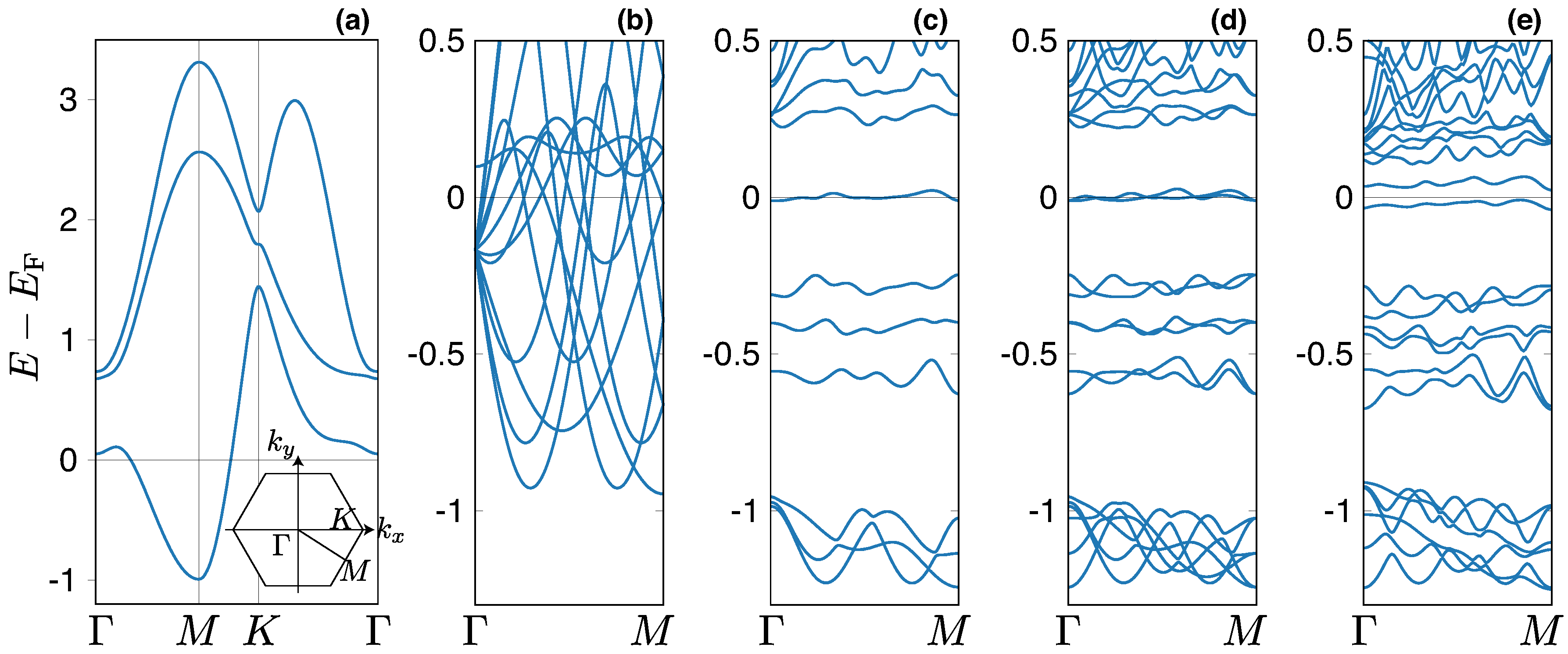
The band structure in our tight-binding model is summarized in Figure 2. Panel (a) shows the result calculated from ${\widehat{H}}_{\mathrm{TB}}^0$ (1) in the absence of a PLD. Panel (b) shows the same result, but the bands are folded by taking a hexagram as a unit cell. Panel (c) shows the result calculated from ${\widehat{H}}_{\mathrm{TB}}$ (3) with distortion $x=-1.5$. This case shows a large band restructuring, and one narrow band separates from the others and extends near the Fermi energy. This isolation becomes clearer for larger $\left|x\right|$ with $x<0$. Note that we consider the case of $x<-1$, while the value $x=-1$ was used in [38] with referring to the experimental values. This is because the value $\left|x\right|=1$ is not large enough to obtain a splitting of the narrow band within our treatment of the electron–electron interactions discussed below. The discrepancy of our value $x=-1.5$ from the experimental one $x=-1.0$ could be decreased if we corrected the approximate law for the transfer integral change (2). In this paper, we do not go into detail in this direction and keep using Equation (2).

2.2. Electron–Electron Interactions

We now add to ${\widehat{H}}_{\mathrm{TB}}$ (3) the electron–electron interactions of on-site Coulomb type

$$\begin{array}{ccc}{\widehat{H}}_{\mathrm{int}}={\displaystyle \sum _i}{\widehat{H}}_{\mathrm{int}}^{\left(i\right)};& {\widehat{H}}_{\mathrm{int}}^{\left(i\right)}=U{\displaystyle \sum _m}{\widehat{n}}_{im\uparrow }{\widehat{n}}_{im\downarrow }+U^{\prime }{\displaystyle \sum _{m\ne m^{\prime }}}{\widehat{n}}_{im\uparrow }{\widehat{n}}_{i{m}^{\prime }\downarrow }+(U^{\prime }-J)& {\displaystyle \sum _{m<m^{\prime },\sigma }}{\widehat{n}}_{im\sigma }{\widehat{n}}_{i{m}^{\prime }\sigma }.\end{array}$$

(5)

Here, we use the standard choice $U^{\prime }=U-2J$ and ignore the pair hopping terms [41]. For simplicity, throughout this paper, we focus on the typical case of $U=3J$, where the last term in Equation (5) vanishes. We use a mean-field approach and approximate ${\widehat{H}}_{\mathrm{int}}^{\left(i\right)}$ by

$${\widehat{H}}_{\mathrm{int}}^{\left(i\right)}\simeq U{\displaystyle \sum _m}\left(n_{im\downarrow }{\widehat{n}}_{im\uparrow }+n_{im\uparrow }{\widehat{n}}_{im\downarrow }-n_{im\uparrow }{n}_{im\downarrow }\right)+U^{\prime }{\displaystyle \sum _{m\ne m^{\prime }}}\left(n_{i{m}^{\prime }\downarrow }{\widehat{n}}_{im\uparrow }+n_{im\uparrow }{\widehat{n}}_{i{m}^{\prime }\downarrow }-n_{im\uparrow }{n}_{i{m}^{\prime }\downarrow }\right),$$

(6)

where $n_{im\sigma }\equiv \langle {\widehat{n}}_{im\sigma }\rangle$ is determined self-consistently and we have neglected the orbital off-diagonal contributions $\langle {\widehat{c}}_{im\sigma }^{†}{\widehat{c}}_{i{m}^{\prime }\sigma }\rangle$ for simplicity.

In the mean-field approximation, we use the unit cell made of two hexagrams, which accommodates 26 electrons, and it is important that the electron number is even. To simulate the charge distribution in the Mott insulator phase, we introduce a fictitious magnetic order in the mean-field approximation. However, this redundant magnetic order is not very harmful when we discuss the charge dynamics driven by strong laser fields. Another drawback is that the translation symmetry is further lowered than a periodic array of hexagrams, but we shall show later that this effect is not very strong.

We compare in Figure 2d,e the band structure without and with the electron–electron interaction. Panel (d) is plotted for comparison and shows the same energy bands as in (c) ($U=3J=0$), but the bands are now folded corresponding to a two-hexagram unit cell. Figure 2e is the result for $U=3J=0.816\mathrm{eV}$ calculated at zero temperature $T=0$ K. The interactions have relatively weak effects at energies well below the Fermi energy $E_F$. However, near $E_F$, they cause a splitting of the two bands and make the system insulating. We have confirmed that these qualitative features remain unchanged for $U=3J\le 2.86\mathrm{eV}$. For $U=3J=0.816\mathrm{eV}$, the band gap at the $\Gamma$ point is 69.2 meV, which is a few times smaller than the experimental value [15]. While the gap size could be reproduced by tuning U, $U^{\prime }$, and J, we do not go into further detail in this paper.

Let us now examine charge and spin densities. The results are shown in Figure 3 for the same parameters $U=3J=0.816\mathrm{eV}$ at $T=0$ K. All the hexagrams have the identical charge–density distribution: the density increases toward the center of each hexagram, and the 2-fold rotational symmetry around an A site is preserved. The 6-fold rotational symmetry is broken due to the doubled unit cell, but its asymmetry is so small (about 1%) that this effect is ignorable. In the doubled unit cell, the two hexagrams have the spin density distribution with the opposite signs, and this is due to a fictitious Neel order. The spin density distribution in each hexagram reflects the profile of the wave functions of the narrow band in Figure 2c. In fact, as was shown in [38], these wave functions have a large amplitude near the hexagram center (A site).

We emphasize again that the spin polarization appears due to the technical reason in treating a Mott insulator by the mean-field approximation (6). We also note that a recent ab initio study by Yi et al. [42] has found a ferromagnetic state to be slightly more stable than the antiferromagnetic one. However, as a matter of fact, the CCDW phase of 1T-TaS${}_2$ is paramagnetic [13,14]. Our aim is not to discuss the spin structure, but to investigate the charge properties, which play the main role upon strong laser drivings. For this purpose, we have now set up a reasonable model by adding the Coulomb interaction (5) to the tight-binding Hamiltonian (3) used in previous studies.

3. Lattice Degree of Freedom

To discuss cooperative phenomena, we now generalize our model and treat the lattice distortion x as a dynamical variable. We discuss its statics in this section and shall do its dynamics in Section 4.

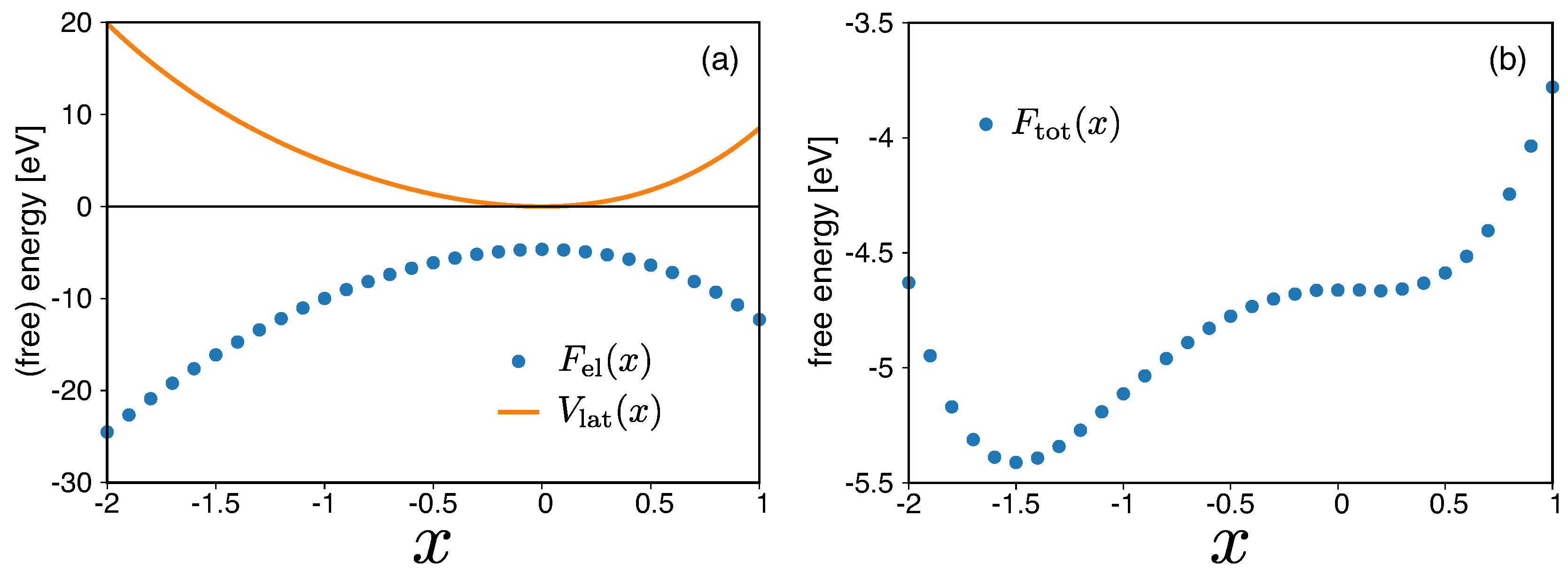
We parametrize the elastic energy per two-hexagram unit cell accompanied by a PLD as

$$V_{\mathrm{lat}}\left(x\right)=\frac{K_2}{2}{x}^2+\frac{K_3}{3}{x}^3+\frac{K_4}{4}{x}^4,$$

(7)

where $K_2,K_3,$ and $K_4$ are positive parameters so that $V_{\mathrm{lat}}\left(x\right)$ is convex. Equation (7) is a Taylor series in x, which starts from $x^2$ since $x=0$ represents the equilibrium position at high temperatures. We take account of the $x^3$ term, since the asymmetry between $x<0$ and $x>0$, or shrinking and expanding hexagrams, become nonnegligible for larger x.

We set the parameters $K_2,K_3,$ and $K_4$ so as to satisfy the following three conditions: (i) the CDW phase appears at $T\sim 500\mathrm{K}$, (ii) $x=-1.5$ in equilibrium at $T=0$ K, and (iii) the free energy difference between the CCDW ($x=-1.5$) and the uniform ($x=0$) states is not very large, or typically less than 1 eV at $T=0$ K per two-hexagram unit cell. Here, the free energy means the sum of $V_{\mathrm{lat}}\left(x\right)$ and the electronic free energy $F_{\mathrm{el}}\left(x\right)$ calculated for ${\widehat{H}}_{\mathrm{TB}}\left(x\right)+{\widehat{H}}_{\mathrm{int}}$ within the mean-field approximation (6). The condition (i) determines $K_2$, and then the conditions (ii) and (iii) do $K_3$ and $K_4$. We have chosen $K_2=12.1$ eV, $K_3=5.44$ eV, and $K_4=2.54$ eV.

Figure 4a shows the electronic energy $F_{\mathrm{el}}\left(x\right)$ at $T=0$ K and $V_{\mathrm{lat}}\left(x\right)$ as functions of x. We note that the free energy coincides with the energy at $T=0$ K. The PLD decreases $F_{\mathrm{el}}\left(x\right)$ and increases $V_{\mathrm{lat}}\left(x\right)$ in both directions $x<0$ and $x>0$. The competition between these gain and cost results in the minimum of the total free energy $F_{\mathrm{el}}\left(x\right)+V_{\mathrm{lat}}\left(x\right)$ at $x=-1.5$ as shown in Figure 4b. There also exists a very shallow local minimum at $x\sim 0.2$ corresponding to an expanding hexagram. At higher temperatures above ∼800 K, the total free energy $F_{\mathrm{el}}\left(x\right)+V_{\mathrm{lat}}\left(x\right)$ has only one minimum at $x=0$ and the CDW is not present. We note that this transition temperature is probably overestimated since we have performed the mean-field approximation (6) and neglected phonon fluctuations.

We make a remark on the simplification that we have made on the PLD. We have treated one specific mode of the hexagram shape in lattice distortion, but the distortion has many more modes. In fact, 1T-TaS${}_2$ shows an incommensurate CDW below 540 K and a nearly commensurate CDW below 350 K, which cannot be described within the present model. Thus, we do not further discuss the free energy at intermediate temperatures, and shall focus on the CCDW state thus obtained at $T=0$ K.

4. Photoinduced Dynamics

4.1. Equations of Motion

To study the photoinduced charge dynamics, we use the coupled equations of motion for the electrons and the PLD. We treat the electrons quantum-mechanically and describe their state by a mean-field wave function $|\mathsf{\Psi }\left(t\right)\rangle$ at each time t. For the PLD, we classically treat it and describe its coordinate and momentum, $x\left(t\right)$ and $p\left(t\right)$, by Hamilton’s equations of motion.

The total Hamiltonian is given by

$$\begin{array}{c}{\widehat{H}}_{\mathrm{total}}={\widehat{H}}_{\mathrm{el}}(x\left(t\right),t)+H_{\mathrm{lat}}(x\left(t\right),p\left(t\right)),\hfill \end{array}$$

(8)

$$\begin{array}{c}{\widehat{H}}_{\mathrm{el}}(x\left(t\right),t)\equiv {\widehat{H}}_{\mathrm{TB}}(x\left(t\right),t)+{\widehat{H}}_{\mathrm{int}},\hfill \end{array}$$

(9)

$$\begin{array}{c}{H}_{\mathrm{lat}}(x\left(t\right),p\left(t\right))\equiv \frac{p{\left(t\right)}^2}{2M}+V_{\mathrm{lat}}\left(x\left(t\right)\right),\hfill \end{array}$$

(10)

where M is the effective mass of the PLD and its value will be discussed later, and ${\widehat{H}}_{\mathrm{int}}$ is treated within the mean-field approximation (6). The explicit time dependence of ${\widehat{H}}_{\mathrm{TB}}(x\left(t\right),t)$ comes from the coupling to the laser electric field, which oscillates in time. We assume that the electric field $\mathit{E}\left(t\right)$ is spatially uniform and treat it in terms of the vector potential $\mathit{A}\left(t\right)$ satisfying $\mathit{E}\left(t\right)=-\mathrm{d}\mathit{A}\left(t\right)/\mathrm{d}t$. Then, ${\widehat{H}}_{\mathrm{TB}}(x\left(t\right),t)$ is obtained from Equation (3) with the Peierls substitution

$$t_{m{m}^{\prime }}^{ij}\left(\left\{{\mathit{r}}_i\left(t\right)\right\}\right)\to t_{m{m}^{\prime }}^{ij}\left(\left\{{\mathit{r}}_i\left(t\right)\right\}\right)exp\left[\mathrm{i}({\mathit{r}}_i\left(t\right)-{\mathit{r}}_j\left(t\right))·\mathit{A}\left(t\right)\right],$$

(11)

where the elementary charge is set to unity.

The equations of motion are given by

$$\begin{array}{c}\mathrm{i}\hslash \frac{\mathrm{d}}{\mathrm{d}t}|\mathsf{\Psi }\left(t\right)\rangle ={\widehat{H}}_{\mathrm{el}}(x\left(t\right),t)|\mathsf{\Psi }\left(t\right)\rangle ,\hfill \end{array}$$

(12)

$$\begin{array}{c}\frac{\mathrm{d}x\left(t\right)}{\mathrm{d}t}=\frac{p\left(t\right)}{M},\hfill \end{array}$$

(13)

$$\begin{array}{c}\frac{\mathrm{d}p\left(t\right)}{\mathrm{d}t}=-\frac{\mathrm{d}{V}_{\mathrm{lat}}\left(x\left(t\right)\right)}{\mathrm{d}x}-\langle \mathsf{\Psi }\left(t\right)|\frac{\partial {\widehat{H}}_{\mathrm{el}}(x\left(t\right),t)}{\partial x}|\mathsf{\Psi }\left(t\right)\rangle .\hfill \end{array}$$

(14)

In the Schrödinger Equation (12), we have ignored the c-number term $H_{\mathrm{lat}}(x,p)$ on the right-hand side since it affects no physical observables. Equations (13) and (14) are Hamilton’s equations of motion for the PLD. The right-hand side of Equation (14) represents the force acting on the PLD and consists of the elasticity and the reaction from the electrons. We note that, when $\mathit{E}\left(t\right)=0$, ${\widehat{H}}_{\mathrm{el}}(x\left(t\right),t)$ does not depend explicitly on t and the total energy $\langle \mathsf{\Psi }\left(t\right)|{\widehat{H}}_{\mathrm{el}}\left(x\left(t\right)\right)|\mathsf{\Psi }\left(t\right)\rangle +H_{\mathrm{lat}}(x\left(t\right),p\left(t\right))$ is a conserved quantity. In solving these equations, we invoke the standard Runge–Kutta method and take a sufficiently small time step to ensure that the norm of the wave function is conserved as good as 8 digits.

4.2. Cooperative Dynamics of Charge and Lattice

Motivated by recent experiments, we study the electronic excitation driven by an ultrashort laser pulse. We take the following form for the vector potential:

$$\mathit{A}\left(t\right)=\mathit{ϵ}{A}_{0}cos\left({\omega }_{\mathrm{pump}}t\right)exp\left(-\frac{t^2}{2T_{\mathrm{pump}}^2}\right).$$

(15)

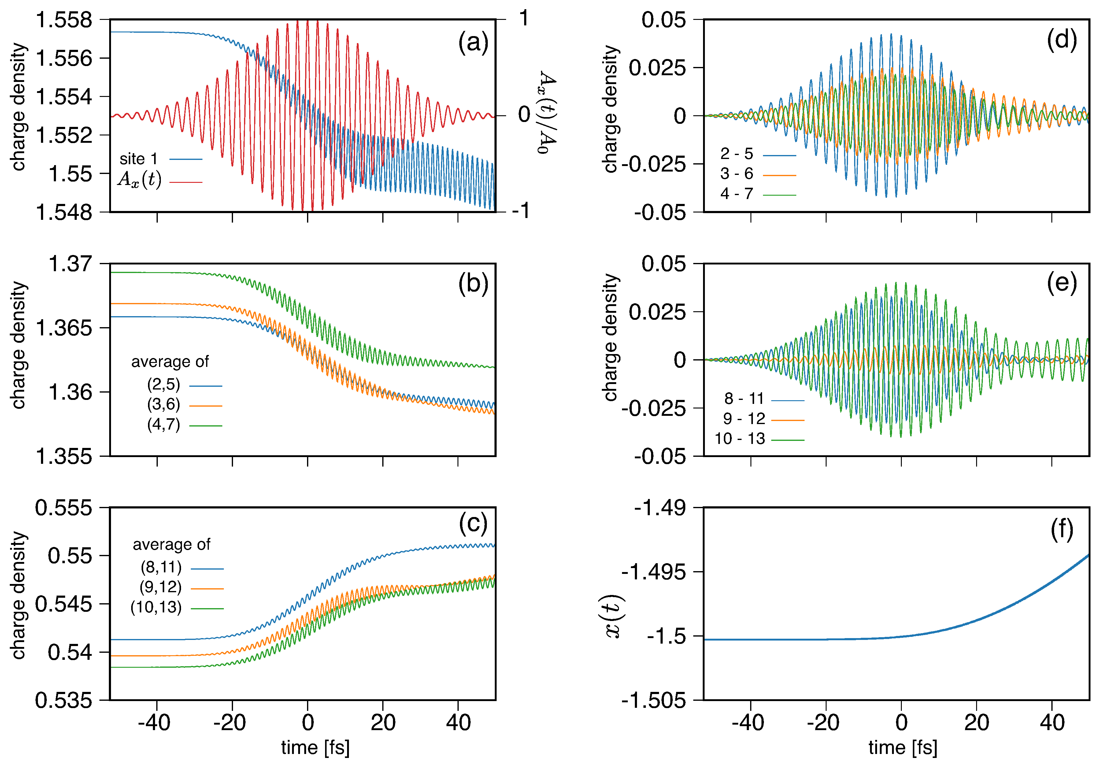
Here, the real parameter $A_0$ denotes the peak amplitude of the vector potential, and $\mathit{ϵ}$ is the polarization vector and assumed to be $\mathit{ϵ}=(1,0)$ in this paper. The results are not sensitive to the direction of $\mathit{ϵ}$. Following the experiment [20], we set the central frequency ${\omega }_{\mathrm{pump}}$ and the pulse width $T_{\mathrm{pump}}$ so that $\hslash {\omega }_{\mathrm{pump}}=1.55\mathrm{eV}$ and $2T_{\mathrm{pump}}=35\mathrm{fs}$. The profile $A_x\left(t\right)$ is shown in Figure 5a. We note that the peak amplitude of the electric field is approximately given by $E_0={\omega }_{\mathrm{pump}}{A}_0$ since $T_{\mathrm{pump}}\gg 1/{\omega }_{\mathrm{pump}}=2.4\mathrm{fs}$. In the following, we shall use $E_0$ rather than $A_0$, making it easier to compare our results with experimental results.

The laser electric field induces charge dynamics on a short time scale of order $T_{\mathrm{pump}}$. In Figure 5, we show the numerical results of local charge densities at 13 sites in a hexagram unit for a typical peak amplitude of the electric field $E_0=0.92\mathrm{MV}/\mathrm{cm}$, which is comparable with the experimental condition [20] (see Figure 1 for the labeling of sites). Since we are not interested in the spin density, the charge density averaged between the two hexagrams is plotted. At our initial time of calculation $t=t_{\mathrm{init}}=-52.5\mathrm{fs}$, the charge–density distribution is the one shown in Figure 3a. As noted before, the 6-fold rotational symmetry is slightly broken down to the 2-fold symmetry. As time advances, the electric field envelope gradually increases, and the charge density starts to oscillate in time at each site.

To analyze the charge-density oscillations in detail, we pair up the six “B” sites as $(2,5)$, $(3,6)$, and $(4,7)$, each of which locates symmetrically about the central A site. We do the similar pairing for the “C” sites as well. We look into the average and the difference of the charge densities for each site pair, which are even and odd, respectively, under the 2-fold rotation. We note that the charge density at site 1 (A) itself is even under this operation. These even and odd quantities show different kinds of dynamics. The even quantities shown in panels (a–c) oscillate with frequency ∼2${\omega }_{\mathrm{pump}}$, whereas the odd ones (d,e) do with frequency $\sim {\omega }_{\mathrm{pump}}$. This is because the vector potential $\mathit{A}\left(t\right)$ has an odd parity with respect to the 2-fold rotation, and these two quantities are coupled to $\mathit{A}\left(t\right)$ in the second and the first orders, respectively.

In addition to those oscillations, the charge dynamics changes its spatial distribution and the CDW order decreases on the short time scale of order $T_{\mathrm{pump}}$. The charge-density imbalance in panels (a–c) decreases during the laser irradiation, and the local charge density slightly approaches the uniform one.

This CDW order decrease is caused not just by the decrease in the PLD. Figure 5f shows that the lattice distortion $x\left(t\right)$ remains almost unchanged until $t\sim 0$, while the significant changes have already appeared in the charge density. In addition, at $0<t<50\mathrm{fs}$, $\left|x\right(t\left)\right|$ gradually decreases, while the charge dynamics rather slows down. Therefore, the short-time dynamics is dominated by the electrons driven by the laser field, and the CDW is rapidly suppressed.

On a longer time scale, the lattice distortion $x\left(t\right)$ plays the main role in dynamics. We show $x\left(t\right)$ up to $t=1000\mathrm{fs}$ in Figure 6. Its time evolution is well approximated by a harmonic oscillation starting at $t\sim 0\mathrm{fs}$, and its frequency is determined as $2.14\mathrm{THz}$ by a sinusoidal fitting. This agrees well with the experimentally observed value $2.1\mathrm{THz}$ of the coherent phonon [16]. Of course, the frequency depends on the effective mass M of the PLD. The smaller M is chosen, the faster the lattice motion becomes. We have set $M=8.00\times {10}^3\mathrm{u}$ in the unified atomic mass unit to make the frequency consistent with the experimental result.

The lattice dynamics can be interpreted by an instantaneous modulation of the free energy profile as schematically illustrated in Figure 6b. In the initial state, the lattice distortion x is located at the minimum of the total free energy $F_{\mathrm{eq}}$. Then, on the short time scale, the laser drives the electrons to a high-energy state, and the free energy is changed into a new one $F_{\mathrm{neq}}$, whose minimum shifts toward $x=0$. Since the lattice distortion remains almost unchanged during the driving, the free energy is not minimum and the distortion x oscillates harmonically around the new minimum of the free energy.

We remark that the harmonic oscillation is not damped in our model since we incorporate no dissipation processes and the total energy is conserved. In reality, the time scale of the damping is known to be $\sim 4$ ps. Thus, we do not proceed with our analysis after $t\sim 1000\mathrm{fs}$, where dissipation would start to play an important role in dynamics.

We briefly summarize the cooperative dynamics revealed by our analysis. The short-time dynamics are dominated by the electronic degrees of freedom driven by the laser. The driving rapidly suppresses the CDW order on the time scale of the pulse width, which is $35\mathrm{fs}$ in our analysis. In this time scale, the PLD is approximately frozen and does not decrease much. On the long time scale of order $100\mathrm{fs}$, the PLD starts to oscillate at frequency $\sim 2\mathrm{THz}$ and will be damped in general through dissipation. These observations are consistent with the experimental finding [16], which observed a delay of the PLD decrease after the CDW order decrease.

4.3. Melting of Hexagrams

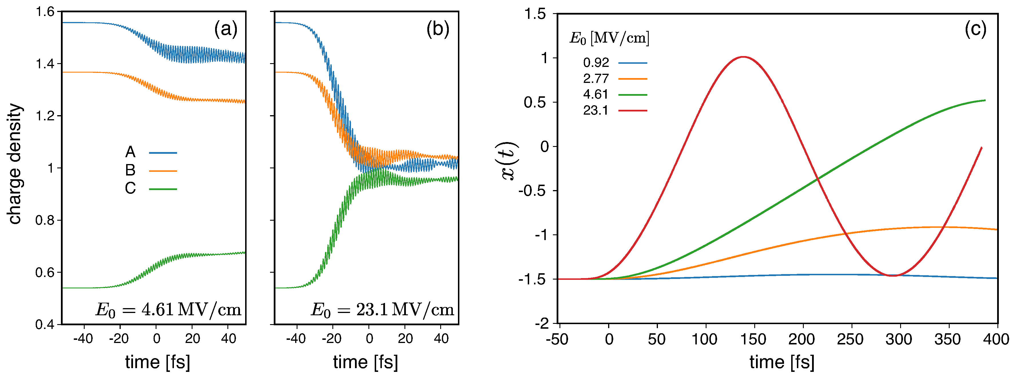
Now, we further increase the laser amplitude and see how the lattice dynamics changes. Figure 7 shows the dynamics of the charge densities averaged over A, B, and C sites for the larger peak amplitudes $E_0=4.61$ and $23.1\mathrm{MV}/\mathrm{cm}$ in panels (a,b), respectively. For $E_0=4.61\mathrm{MV}/\mathrm{cm}$, the CDW order decreases by $\sim 20\%$, which is much enhanced than the case of $E_0=0.92\mathrm{MV}/\mathrm{cm}$ shown in Figure 5. For $E_0=23.1\mathrm{MV}/\mathrm{cm}$, the CDW order disappears and the charge distribution becomes nearly uniform within $\sim 20\mathrm{fs}$. We note that the PLD remains present on this time scale as shown in panel (c). Only the CDW order of the hexagram shape melts down on the short time scale.

Next, we discuss the energy efficiency of the photoinduced CDW melting. We have calculated the energy absorption $\Delta E_{\mathrm{abs}}\equiv E(t=0\mathrm{fs})-E_{\mathrm{init}}$, and obtained $\Delta E_{\mathrm{abs}}=4.6$ and $39\mathrm{eV}$ per two hexagrams for $E_0=4.61$ and $23.1\mathrm{MV}/\mathrm{cm}$, respectively. We compare these values with the energy difference $\Delta E_{\mathrm{CDW}}\equiv E_{\mathrm{uniform}}-E_{\mathrm{init}}$. Here, $E_{\mathrm{uniform}}$ denotes the energy of a virtual uniform state and is defined as the expectation value of ${\widehat{H}}_{\mathrm{total}}$ (8) at $x=-1.5$ calculated for the electronic ground state of ${\widehat{H}}_{\mathrm{total}}$ for $x=0$. We obtain $\Delta E_{\mathrm{CDW}}=5.8\mathrm{eV}$ per two hexagrams, and it is an estimate of the energy needed to wash out the CDW order without deforming the PLD. It is consistent with the fact that $\Delta E_{\mathrm{abs}}<\Delta E_{\mathrm{CDW}}$ for $E_0=4.61\mathrm{MV}/\mathrm{cm}$, where the CDW is suppressed but remains, whereas $\Delta E_{\mathrm{abs}}>\Delta E_{\mathrm{CDW}}=0.15\Delta E_{\mathrm{abs}}$ for $E_0=23.1\mathrm{MV}/\mathrm{cm}$, where the CDW melts down. Thus, $15\%$ of the absorbed energy is used for the CDW melting, and the remaining $85\%$ is converted into heat.

To melt the CDW order, the laser–electron interaction is not the only way since the lattice motion is involved on the long time scale. We show the lattice dynamics in Figure 7 for some strong laser fields. For $E_0=4.61\mathrm{MV}/\mathrm{cm}$, $x\left(t\right)$ hits zero, meaning that the PLD of the hexagram shape melts down and the CDW order of electrons thereby disappears. We note that this field amplitude is not strong enough to completely melt the CDW order on the short time scale. However, in the long run, the laser energy absorbed by the electrons is transferred to the lattice motion, which affects the charge density through the electron–lattice coupling. On the long time scale, the electron–lattice cooperative dynamics becomes more important.

These electron–lattice dynamics are quite different from those found in experimental [43] and theoretical studies [44,45] on charge order melting in quasi-two-dimensional organic conductors. In these materials, the charge order is mainly produced by long-range Coulomb repulsion and weakly assisted by an electron–lattice coupling. Thus, the charge order can be melted efficiently by a pulse laser with little changing the lattice distortion. See also [46] for the efficiency of the charge order melting in a quasi-one-dimensional organic conductor.

5. Summary and Discussion

In this work, we have extended the tight-binding model (3) of the previous studies [37,38] and included the on-site Coulomb interactions (5). By this extension and our mean-field analysis, we have succeeded in opening a band gap at the Fermi level as shown in Figure 2e. Thus, we have established a lattice model which reproduces qualitative features of the electronic properties of 1T-TaS${}_2$. We have further extended the model to treat the lattice distortion as a dynamical variable. Considering a specific PLD of the hexagram shape, we have modeled the lattice potential, reproduced the CCDW as a thermal equilibrium state, and formulated the coupled equations of motion for the electrons and the PLD.

We have investigated the short-time charge dynamics induced by a pulse laser on the basis of our model. We have shown that the short-time dynamics are dominated by electrons and the hexagram CDW order is suppressed by the laser, while the lattice is effectively frozen. This CDW decrease is caused at the second order of the laser electric field, and the CDW order melts down as fast as $20\mathrm{fs}$ for the strong laser amplitude $E_0=23.1\mathrm{MV}/\mathrm{cm}$ for the $35\mathrm{fs}$ pulse. We note that the necessary amplitude $E_0$ should be smaller for a longer pulse.

The lattice distortion plays an important role on the long time scale ≳100 fs. Its motion is dominated by the landscape of the free energy instantaneously converted from the equilibrium one (see Figure 6b). The CDW order may be washed out on the long time scale through the coupling to the lattice motion, even when the laser amplitude is not strong enough to melt the CDW on the short time scale.

We comment on a few open questions beyond our present study. We have considered only one mode of the hexagram shape in lattice distortion, but there exist many other modes giving rise to the incommensurate CDW, the nearly-commensurate CDW, and so on. Including those relevant modes may make it possible to describe photoinduced transitions from the CCDW to the other CDW phases. In that case, our picture of the free-energy modulation is extended in multiple dimensions and several local minima may exist. We note that the phonon modes also work as a heat reservoir. Our present analysis does not include a coupling to any reservoir, or dissipation, and our results would be modified especially at long times. We leave these important issues as future works.

6. Materials and Methods

6.1. Spin–Orbit Interaction

We give the the expressions for ${\widehat{\mathit{L}}}_i$ and ${\widehat{\mathit{S}}}_i$:

$${\widehat{L}}_i^{\alpha }=\sum _{m,m^{\prime },\sigma }{L}_{m{m}^{\prime }}^{\alpha }{\widehat{c}}_{im\sigma }^{†}{\widehat{c}}_{i{m}^{\prime }\sigma };{\widehat{S}}_i^{\alpha }=\frac{1}{2}\sum _{m,\sigma ,{\sigma }^{\prime }}{\tau }_{\sigma {\sigma }^{\prime }}^{\alpha }{\widehat{c}}_{im\sigma }^{†}{\widehat{c}}_{im{\sigma }^{\prime }}(\alpha =x,y,z).$$

(16)

Here, ${\tau }^{\alpha }$’s are the Pauli matrices and $L_{m{m}^{\prime }}^{\alpha }$’s are the $3\times 3$ sub-matrices for $m=$ $3z^2-r^2$, $x^2-y^2$, $xy$ of the $L=2$ representation of the angular momentum [47]. We note that only ${\widehat{L}}_i^z{\widehat{S}}_i^z$ is active in ${\widehat{\mathit{L}}}_i·{\widehat{\mathit{S}}}_i$ within our subspace spanned by the states with $L_i^z=0,\pm 2$. The nonzero elements of $L^z$ are thus $L_{x^2-y^2,xy}^z=-L_{xy,x^2-y^2}^z=\mathrm{i}$.

References

- Wilson, J.A.; Di Salvo, F J.; Mahajan, S. Charge-density waves and superlattices in the metallic layered transition metal dichalcogenides. Adv. Phys. 1975, 24, 117–201. [Google Scholar] [CrossRef]
- Rossnagel, K. On the origin of charge-density waves in select layered transition-metal dichalcogenides. J. Phys. Condens. Matter 2011, 23, 213001. [Google Scholar] [CrossRef] [PubMed]
- Chhowalla, M.; Shin, H.S.; Eda, G.; Li, J.-L.; Loh, K.P.; Zhang, H. The chemistry of two-dimensional layered transition metal dichalcogenide nanosheets. Nat. Chem. 2013, 5, 263–275. [Google Scholar] [CrossRef] [PubMed]
- Wilson, J.A.; Di Salvo, F.J.; Mahajan, S. Charge-Density Waves in Metallic, Layered, Transition-Metal Dichalcogenides. Phys. Rev. Lett. 1974, 32, 882–885. [Google Scholar] [CrossRef]
- Scruby, C.B.; Williams, P.M.; Parry, G.S. The role of charge density waves in structural transformations of 1T-TaS2. Philos. Mag. 1975, 31, 255–274. [Google Scholar] [CrossRef]
- Fung, K.K.; Steeds, J.W.; Eades, J.A. Application of convergent beam electron diffraction to study the stacking of layers in transition-metal dichalcogenides. Physica B 1980, 99, 47–50. [Google Scholar] [CrossRef]
- Tanda, S.; Sambongi, T.; Tani, T.; Tanaka, S. X-ray Study of Charge Density Wave Structure in 1T-TaS2. J. Phys. Soc. Jpn. 1984, 53, 476–479. [Google Scholar] [CrossRef]
- Sakabe, D.; Liu, Z.; Suenaga, K.; Nakatsugawa, K.; Tanda, S. Direct observation of mono-layer, bi-layer, and tri-layer charge density waves in 1T-TaS2 by transmission electron microscopy without a substrate. npj Quantum Mat. 2017, 2, 22. [Google Scholar] [CrossRef]
- Ang, R.; Tanaka, Y.; Ieki, E.; Nakayama, K.; Sato, T.; Li, L.J.; Lu, W.J.; Sun, Y.P.; Takahashi, T. Real-Space Coexistence of the Melted Mott State and Superconductivity in Fe-Substituted 1T-TaS2. Phys. Rev. Lett. 2012, 109, 176403. [Google Scholar] [CrossRef]
- Fazekas, P.; Tosatti, E. Electrical, structural and magnetic properties of pure and doped 1T-TaS2. Philos. Mag. B 1979, 39, 229–244. [Google Scholar] [CrossRef]
- Perfetti, L.; Gloor, T.A.; Mila, F.; Berger, H.; Grioni, M. Unexpected periodicity in the quasi-two-dimensional Mott insulator 1T-TaS2 revealed by angle-resolved photoemission. Phys. Rev. B 2005, 71, 153101. [Google Scholar] [CrossRef]
- Ritschel, T.; Trinckauf, J.; Koepernik, K.; Büchner, B.; Zimmermann, M.V.; Berger, H.; Joe, Y.I.; Abbamonte, P.; Geck, J. Orbital textures and charge density waves in transition metal dichalcogenides. Nat. Phys. 2015, 11, 328–331. [Google Scholar] [CrossRef] [Green Version]
- Law, K.T.; Lee, P.A. 1T-TaS2 as a quantum spin liquid. Proc. Natl. Acad. Sci. USA 2017, 114, 6996–7000. [Google Scholar] [CrossRef] [PubMed]
- Klanjšek, M.; Zorko, A.; Zitko, R.; Mravlje, J.; Jaglicic, Z.; Biswas, P.K.; Prelovsek, P.; Mihailovic, D.; Arcon, D. A high-temperature quantum spin liquid with polaron spins. Nat. Phys. 2017, 13, 1130–1134. [Google Scholar] [CrossRef] [Green Version]
- Perfetti, L.; Loukakos, P.A.; Lisowski, M.; Bovensiepen, U.; Wolf, M.; Berger, H.; Biermann, S. Femtosecond dynamics of electronic states in the Mott insulator 1T-TaS2 by time resolved photoelectron spectroscopy. New J. Phys. 2008, 10, 053019. [Google Scholar] [CrossRef]
- Eichberger, M.; Schäfer, H.; Krumova, M.; Beyer, M.; Demsar, J.; Berger, H.; Moriena, G.; Sciaini, G.; Miller, R.J.D. Snapshots of cooperative atomic motions in the optical suppression of charge density waves. Nature 2010, 468, 799–802. [Google Scholar] [CrossRef] [Green Version]
- Ishizaka, K.; Kiss, T.; Yamamoto, T.; Ishida, Y.; Saitoh, T.; Matsunami, M.; Eguchi, R.; Ohtsuki, T.; Kosuge, A.; Kanai, T.; et al. Femtosecond core-level photoemision spectroscopy on 1T-TaS2 using a 60-eV laser source. Phys. Rev. B 2011, 83, 081104. [Google Scholar] [CrossRef]
- Hellmann, S.; Rohwer, T.; Kalläne, M.; Hanff, K.; Sohrt, C.; Stange, A.; Carr, A.; Murnane, M.M.; Kapteyn, H.C.; Kipp, L.; et al. Time-domain classification of charge-density-wave insulators. Nat. Commun. 2012, 3, 1069. [Google Scholar] [CrossRef] [Green Version]
- Haupt, K.; Eichberger, M.; Erasmus, N.; Rohwer, A.; Demsar, J.; Rossnagel, K.; Schwoerer, H. Ultrafast Metamorphosis of a Complex Charge-Density Wave. Phys. Rev. Lett. 2016, 116, 016402. [Google Scholar] [CrossRef]
- Stojchevska, L.; Vaskivskyi, I.; Mertelj, T.; Kusar, P.; Svetin, D.; Brazovskii, S.; Mihailovic, D. Ultrafast Switching to a Stable Hidden Quantum State in an Electronic Crystal. Science 2014, 344, 177–180. [Google Scholar] [CrossRef] [Green Version]
- Gerasimenko, Y.A.; Vaskivskyi, I.; Mihailovic, D. Dual vortex charge order in a metastable state created by an ultrafast topological transition in 1T-TaS2. arXiv, 2017; arXiv:1704.08149. [Google Scholar]
- Ravnik, J.; Vaskivskyi, I.; Mertelj, T.; Mihailovic, D. Real-time observation of the coherent transition to a metastable emergent state in 1T-TaS2. Phys. Rev. B 2018, 97, 075304. [Google Scholar] [CrossRef]
- Sun, K.; Sun, S.; Zhu, C.; Tian, H.; Yang, H.; Li, J. Hidden CDW states and insulator-to-metal transition after a pulsed femtosecond laser excitation in layered chalcogenide 1T-TaS2−xSex. Sci. Adv. 2018, 4, eaas9660. [Google Scholar] [CrossRef] [PubMed]
- Stojchevska, L.; Šutar, P.; Goreshnik, E.; Mihailovic, D.; Mertelj, T. Optical creation and temperature stability of the hidden charge density wave state in 1T-TaS2−xSex. arXiv, 2018; arXiv:1806.03094. [Google Scholar]
- Yoshida, M.; Zhang, Y.; Ye, J.; Suzuki, R.; Imai, Y.; Kimura, S.; Fujiwara, A.; Iwasa, Y. Controlling charge-density-wave states in nano-thick crystals of 1T-TaS2. Sci. Rep. 2014, 4, 7302. [Google Scholar] [CrossRef] [PubMed]
- Yoshida, M.; Suzuki, R.; Zhang, Y.; Nakano, M.; Iwasa, Y. Memristive phase switching in two-dimensional 1T-TaS2 crystals. Sci. Adv. 2015, 1, e1500606. [Google Scholar] [CrossRef] [PubMed]
- Yoshida, M.; Gokuden, T.; Suzuki, R.; Nakano, M.; Iwasa, Y. Current switching of electronic structures in two-dimensional 1T-TaS2 crystals. Phys. Rev. B 2017, 95, 121405(R). [Google Scholar] [CrossRef]
- Vaskivskyi, I.; Mihailovic, I.A.; Brazovskii, S.; Gospodaric, J.; Mertelj, T.; Svetin, D.; Sutar, P.; Mihailovic, D. Fast electronic resistance switching involving hidden charge density wave states. Nat. Commun. 2016, 7, 11442. [Google Scholar] [CrossRef] [Green Version]
- Ichikawa, H.; Nozawa, S.; Sato, T.; Tomita, A.; Ichiyanagi, K.; Chollet, M.; Guerin, L.; Dean, N.; Cavalleri, A.; Adachi, S.; et al. Transient photoinduced ‘hidden’ phase in a manganite. Nat. Mater. 2011, 10, 101–105. [Google Scholar] [CrossRef]
- Beaud, P.; Caviezel, A.; Mariager, S.O.; Rettig, L.; Ingold, G.; Dornes, C.; Huang, S.-W.; Johnson, J.A.; Radovic, M.; Huber, T.; et al. A time-dependent order parameter for ultrafast photoinduced phase transitions. Nat. Mater. 2014, 13, 923–927. [Google Scholar] [CrossRef]
- Li, J.; Strand, H.U.R.; Werner, P.; Eckstein, M. Theory of photoinduced ultrafast switching to a spin–orbital ordered hidden phase. Nat. Commun. 2018, 9, 4581. [Google Scholar] [CrossRef]
- Wu, D.; Ma, Y.; Niu, Y.; Liu, Q.; Dong, T.; Zhang, S.; Niu, J.; Zhou, H.; Wei, J.; Wang, Y.; Zhao, Z.; Wang, N. Ultrabroadband photosensitivity from visible to terahertz at room temperature. Sci. Adv. 2018, 4, eaao3057. [Google Scholar] [CrossRef] [PubMed]
- McMillan, W.L. Theory of discommensurations and the commensurate-incommensurate charge-density-wave phase transition. Phys. Rev. B 1976, 14, 1496–1502. [Google Scholar] [CrossRef]
- Moncton, D.E.; Axe, J.D.; DiSalvo, F.J. Neutron scattering study of the charge-density wave transitions in 2H-TaSe2 and 2H-NbSe2. Phys. Rev. B 1977, 16, 801–819. [Google Scholar] [CrossRef]
- Nakanishi, K.; Shiba, H. Domain-like Incommensurate Charge-Density-Wave States and the First-Order Incommensurate-Commensurate Transitions in Layered Tantalum Dichalcogenides. I. 1T-Polytype. J. Phys. Soc. Jpn. 1977, 43, 1839–1847. [Google Scholar] [CrossRef]
- Mattheiss, L.F. Band Structures of Transition-Metal-Dichalcogenide Layer Compounds. Phys. Rev. B 1973, 8, 3719–3740. [Google Scholar] [CrossRef]
- Smith, N.V.; Kevan, S.D.; DiSalvo, F.J. Band structures of the layer compounds 1T-TaS2, and 2H-TaSe2 in the presence of commensurate charge-density waves. J. Phys. C Solid State Phys. 1985, 18, 3175–3189. [Google Scholar] [CrossRef]
- Rossnagel, K.; Smith, N.V. Spin-orbit coupling in the band structure of reconstructed 1T-TaS2. Phys. Rev. B 2006, 73, 073106. [Google Scholar] [CrossRef]
- Slater, J.C.; Koster, G.F. Simplified LCAO Method for the Periodic Potential Problem. Phys. Rev. 1954, 94, 1498–1524. [Google Scholar] [CrossRef]
- Miasek, M. Tight-Binding Method for Hexagonal Close-Packed Structure. Phys. Rev. 1957, 107, 92–95. [Google Scholar] [CrossRef]
- Kanamori, J. Electron Correlation and Ferromagnetism of Transition Metals. Prog. Theory Phys. 1963, 30, 275–289. [Google Scholar] [CrossRef] [Green Version]
- Yi, S.; Zhang, Z.; Cho, J.-H. Coupling of charge, lattice, orbital, and spin degrees of freedom in charge density waves in 1T-TaS2. Phys. Rev. B 2018, 97, 041413. [Google Scholar] [CrossRef]
- Iwai, S.; Yamamoto, K.; Kashiwazaki, A.; Hiramatsu, F.; Nakaya, H.; Kawakami, Y.; Yakushi, K.; Okamoto, H.; Mori, H.; Nishio, Y. Photoinduced Melting of a Stripe-Type Charge-Order and Metallic Domain Formation in a Layered BEDT-TTF-Based Organic Salt. Phys. Rev. Lett. 2007, 98, 097402. [Google Scholar] [CrossRef] [PubMed]
- Tanaka, Y.; Yonemitsu, K. Growth Dynamics of Photoinduced Domains in Two-Dimensional Charge-Ordered Conductors Depending on Stabilization Mechanisms. J. Phys. Soc. Jpn. 2010, 79, 024712. [Google Scholar] [CrossRef] [Green Version]
- Miyashita, S.; Tanaka, Y.; Iwai, S.; Yonemitsu, K. Charge, Lattice, and Spin Dynamics in Photoinduced Phase Transitions from Charge-Ordered Insulator to Metal in Quasi-Two-Dimensional Organic Conductors. J. Phys. Soc. Jpn. 2010, 79, 034708. [Google Scholar] [CrossRef] [Green Version]
- Yonemitsu, K.; Maeshima, N. Photoinduced melting of charge order in a quarter-filled electron system coupled with different types of phonons. Phys. Rev. B 2010, 76, 075105. [Google Scholar] [CrossRef]
- Sakurai, J.J. Modern Quantum Mechanics; Revised ed.; Addison Wesley: Boston, MA, USA, 1993; ISBN 978-0201539295. [Google Scholar]
Figure 1.
(a) PLD in hexagram configuration in real space (exaggerated). The red, blue, and orange dots show “A”, “B”, and “C” Ta atoms, respectively. For reference, Ta atoms without PLD are shown by the gray dots; (b) parameters and characterizing distorted hexagram configuration. The configuration is assumed to be symmetric under the rotation and the mirror transformation about the x-axis. The site indices will be used in Section 4.
Figure 2.
(a) band structure without PLD or Coulomb interaction. The inset schematically shows the Brillouin zone; (b) the same result with folded bands obtained by taking each hexagram as a unit cell; (c) band structure with PLD () and no Coulomb interaction; (d) the same result shown with folded bands for two-hexagram unit cell; (e) band structure with both PLD () and on-site Coulomb interaction () calculated within mean-field approximation (6) at K.
Figure 3.
Charge (a) and spin (b) densities in two-hexagram unit cell in presence of both PLD () and Coulomb interaction () calculated within mean-field approximation at K. The charge–density distributions of the two hexagrams are identical, whereas their spin–density distributions have opposite signs.
Figure 4.
(a) electronic free energy and elastic energy accompanied by PLD. These values are per two-hexagram unit cell and is calculated for at K; (b) total free energy calculated from data in panel (a).
Figure 5.
Dynamics results for on short time scale. (a) shows the charge density at A site (i.e., site 1) (see Figure 1b for the site index), and the input vector potential (Equation (15)); (b,c) show the time profiles of the average charge density for the pairs of the “B” sites [, , and ], and the “C” sites [, , and ], respectively; (d,e) show those of charge-density difference in the pairs of the “B” sites [, , and ], and the “C” sites [, , and ], respectively; (f) shows the time evolution of the lattice distortion .
Figure 6.
(a) time profile of lattice distortion (solid) and its sinusoidal fitting (dashed); (b) schematic illustration of mechanism of lattice dynamics .
Figure 7.
Time profiles of charge densities averaged over A, B, and C sites for laser amplitudes (a) and (b) ; (c) time profile of lattice distortion for several laser amplitudes .