Attoclock Ptychography

Abstract

Dedicated simulations show that the application of time-domain ptychography to angular photo-electron streaking data allows shot-to-shot reconstruction of individual X-ray free electron laser pulses. Specifically, in this study, we use an extended ptychographic iterative engine to retrieve both the unknown X-ray pulse and the unknown streak field. We evaluate the quality of reconstruction versus spectral resolution, signal-to-noise and sampling size of the spectrogram.

1. Introduction

Time-domain ptychography refers to a specific class of iterative algorithms that reconstruct a complex valued waveform $E(t)$ from a spectrogram,

$$S(\tau ,\omega )\propto {\left|\underset{-\infty }{\overset{\infty }{\int }}\mathrm{d}tE(t)P(t-\tau ){\mathrm{e}}^{-\mathrm{i}\omega t}\right|}^2,$$

(1)

with a known or unknown gate, $P(t)$. The spectrogram itself is composed of spectra of the product field, $E(t)P(t-\tau )$, recorded for a range of time delays, $\tau$. Time-domain ptychography is derived from space-domain ptychography, which was originally proposed to solve the phase problem in crystallography [1]. The real space image of an unknown object is reconstructed iteratively from a series of far-field diffraction measurements. Each of those is recorded after shifting the object or the coherent illumination beam in the object plane. Far-field diffraction patterns must result from different, yet overlapping, areas of the object. Therefore, subsequent measurements must be transversely shifted by an amount smaller than the spatial extent, the “support” of the illumination beam. We have previously demonstrated that such concepts, including spatial reconstruction algorithms, can be transferred to the time domain [2,3,4,5,6] and thus yield numerous ramifications for ultra-fast optics, imaging and spectroscopy. In the time-domain, ptychography operates in the two conjugate one-dimensional spaces of time and frequency. That is, the two-dimensional real space vector, $\overrightarrow{r}$, and the wave vector, $\overrightarrow{k}$, are substituted by t and $\omega$; the object, $E(\overrightarrow{r})$, and the illumination beam, $P(\overrightarrow{r})$, are substituted by the object waveform, $E(t)$, and a gate, $P(t)$, and instead of far-field diffraction images, $S(\overrightarrow{k})$, spectra, $S(\omega )$, are recorded. Combining the spectra recorded at different time delays, $\tau$, results in a spectrogram, as described by Equation (1).

We have previously demonstrated several applications of time-domain ptychography, for example, characterizing both typical and optically shaped ultrafast laser pulses [2,3] as well as super continuum pulses [6]. We have also used time-domain ptychography to reconstruct single attosecond XUV pulses or trains of attosecond XUV pulses from streaked photo-electron spectra [4]. In photo-electron streaking, attosecond XUV pulses ionize an ensemble of atoms in the presence of an infrared field. The resulting energy spectrum of the photo-electrons released along this so-called streak field polarization direction reveals either excess or diminished kinetic energy, depending on the phase and strength of that streak field. Measured as a function of the time delay between XUV and streak pulse, a detailed theoretical analysis showed that this process can be made to reveal a spectrogram, given certain assumptions. Therefore, time-domain ptychography could be used to reconstruct the XUV pulses from the streaked photo-electron spectrogram.

Photo-electron streaking has become the technique of choice for characterizing pulses emitted by X-ray free electron lasers (XFEL) [7]. Given the fluctuations that are typical of the electron acceleration as well as the stochastic nature of the self-amplification of spontaneous emission (SASE) nature of such sources, single shot measurement, not scanning, must be used for pulse characterization; no two pulses look alike at an FEL. In this manuscript, therefore, we propose a combination of so-called angular streaking [8,9] with time-domain ptychography for the reconstruction of individual SASE X-ray pulses on a shot-to-shot basis.

This manuscript is organized as follows. Section 2 summarizes the theoretical background of time-domain ptychography as applied to angular electron streaking for individual X-ray pulses, describes the X-ray pulse structures generated in a typical XFEL, describes photo-electron streaking with streak fields of different polarization states and discusses the extended ptychographic iterative engine (ePIE). Section 3 combines the ingredients, simulating angular streaking for a number of both idealized and realistic X-ray pulses and reconstructing them using the ePIE algorithm. We then investigate the influence of spectral resolution on the electron kinetic energy measurements as well as the effects of different signal-to-noise values and sampling on the quality of reconstruction. The main goal is to identify the minimum number of electron spectra and the required spectrometer resolution to achieve X-ray pulse reconstruction of sufficient quality.

2. Theory

2.1. XFEL Pulses

Shot-to-shot fluctuations of an electron accelerator cause random variations in the electron bunch momentum phase space. This, in turn, causes consequential variation in the resulting X-ray pulse time-energy distribution. Even if the momentum phase space for different electron bunches is identical, the process of self-amplification of spontaneous emission (SASE) builds up from the vacuum fluctuations and therefore, is stochastic from the start. This leads to multiple longitudinal lasing modes that grow exponentially—modes which do not have a shot-to-shot repeatable relative phase relationship. In the time-domain, this produces sub-spikes that have a duration defined by the longitudinal coherence length [10,11], as if each came from an independent radiation source along the longitudinal dimension of the electron bunch. The result is a stochastic train of individually coherent SASE spikes [12] whose intensity, temporal position and carrier-envelope phase vary randomly from shot-to-shot.

2.2. Electron Streaking

In electron streaking, an ionization pulse, typically in the VUV to X-ray region, ionizes atoms in the presence of an AC streak field [13], and the energy spectrum of the photoelectrons released in the process is measured. With no streak field present and a sufficiently flat ionization cross section, the spectrum of the X-ray pulse is mapped to the photoelectron spectrum. When the streak field is on, the photoelectrons gain or lose kinetic energy depending on their time of birth relative to the streak field oscillations. Recording photoelectron spectra as a function of time delay between the X-ray pulse and the streak field results in a two-dimensional time–frequency distribution, which exhibits wiggles that are synchronized to the streak field oscillations. Ideally, the two-dimensional distribution is formally identical to the spectrogram (1). In order to compute the photoelectron spectrum, first, we calculate the transition amplitude, $a_{\overrightarrow{p}}$, from the ground state to a continuum state characterized by the momentum, $\overrightarrow{p}$. For the sake of simplicity, we use the single active electron approximation, e.g., as published in reference [14] and references therein. At times large enough for the ionization field to vanish, the resulting transition amplitude obtained by means of a first-order perturbation theory is

$$a_{\overrightarrow{p}}=-\frac{\mathrm{i}}{\hslash }\underset{-\infty }{\overset{\infty }{\int }}\mathrm{d}t\overrightarrow{d}[\overrightarrow{p}]{\overrightarrow{E}}_X(t)exp\left[\frac{\mathrm{i}}{\hslash }\left(\frac{|\overrightarrow{p}{|}^2}{2m}+I_p\right)t\right].$$

(2)

Here, ${\overrightarrow{E}}_X(t)$ is the X-ray electric field, $\overrightarrow{d}[\overrightarrow{p}]$ is the dipole transition matrix element from the ground to the continuum state, $|\overrightarrow{p}{|}^2/(2m)$ is the energy of the final continuum state and $I_p$ denotes the ionization potential of the atom. The corresponding photoelectron spectrum is

$$S(|\overrightarrow{p}|)\propto {\left|{\int }_{-\infty }^{\infty }\mathrm{d}t\overrightarrow{d}[\overrightarrow{p}]{\overrightarrow{E}}_X(t)exp\left[\frac{\mathrm{i}}{\hslash }\left(\frac{|\overrightarrow{p}{|}^2}{2m}+I_p\right)t\right]\right|}^2.$$

(3)

From Equations (2) and (3), it can be seen that the spectrum resulting from the transition amplitude, $a_{\overrightarrow{p}}$, is directly connected to the X-ray spectrum, both in phase and amplitude. When the streak field temporally overlaps with the emerging electron wave packet, the photoelectrons are either accelerated or decelerated, and the time dependent vector potential is imprinted on the photoelectron spectrum. This scenario is treated as a strong field approximation where the ionic potential is neglected with respect to the streak field. The transition amplitude, $a_{\overrightarrow{p}}(\tau )$, now a function of time delay, $\tau$, between the two fields, is given by

$$\begin{array}{lll}{a}_{\overrightarrow{p}}(\tau )& =& -\frac{\mathrm{i}}{\hslash }\underset{-\infty }{\overset{\infty }{\int }}\mathrm{d}t\overrightarrow{d}[\overrightarrow{p}+e{\overrightarrow{A}}_S(t)]{\overrightarrow{E}}_X(t-\tau )\hfill \\ & & exp\left\{\frac{\mathrm{i}}{\hslash }\left[I_{p}t-\frac{1}{2m}{\int }_t^{\infty }\mathrm{d}{t}^{\prime }{(\overrightarrow{p}+e{\overrightarrow{A}}_S(t^{\prime }))}^2\right]\right\}.\end{array}$$

(4)

where e denotes the electron charge, $\overrightarrow{p}+e{\overrightarrow{A}}_S(t)$ is the instantaneous momentum of a free electron in the streak field and ${\overrightarrow{A}}_S(t)$ is the vector potential associated with the streak field in the Coulomb gauge with the electric field vector, ${\overrightarrow{E}}_S(t)=-\partial {\overrightarrow{A}}_S/\partial t$. Without the streak field, i.e., ${\overrightarrow{A}}_S(t)=0$, Equation (4) reduces to Equation (2). From Equation (4), the corresponding spectrum is derived, and after rearranging the different terms of the integral in the exponential of Equation (4), we obtain

$$\begin{array}{lll}S(|\overrightarrow{p}|,\tau )& \propto & |\underset{-\infty }{\overset{\infty }{\int }}\mathrm{d}t{\overrightarrow{E}}_X(t-\tau )\overrightarrow{d}[\overrightarrow{p}+e{\overrightarrow{A}}_S(t)]P(t)\hfill \\ & & exp\left[\frac{\mathrm{i}}{\hslash }\left(\frac{|\overrightarrow{p}{|}^2}{2m}+I_p\right)t\right]{|}^2.\hfill \end{array}$$

(5)

Since the number of electrons is conserved, the gate, $P(t)$, is a pure phase gate

$$P(t)=exp\left[-\frac{\mathrm{i}}{\hslash }\underset{t}{\overset{\infty }{\int }}\mathrm{d}{t}^{\prime }\left(\frac{e\overrightarrow{p}·{\overrightarrow{A}}_S(t^{\prime })}{m}+\frac{e^2{|{\overrightarrow{A}}_S(t^{\prime })|}^2}{2m}\right)\right].$$

(6)

The measured electron spectra, $S(|\overrightarrow{p}|,\tau )$, can be readily converted to $S(\omega ,\tau )$. When a constant transition matrix element, $\overrightarrow{d}$, is assumed, which is approximately true for streak fields that are not too high, and a linearly polarized ionization pulse, Equation (5) is the spectrogram of the product field, $E_X(t-\tau )P(t)$, and suitable iterative algorithms may be used to reconstruct the slowly varying envelope of the ionization pulse. In the following text, we derive the gate function for an elliptically polarized laser streak field, which includes a linear or a circular polarized streak field as special cases. The electric field of an elliptically polarized streak pulse can be written as

$${\overrightarrow{E}}_S(t)=E_0(t)\frac{1}{\sqrt{1+{\epsilon }^2}}\left[\widehat{x}cos{\omega }_{0}t+\widehat{y}\epsilon sin{\omega }_{0}t\right]$$

(7)

with the unit vectors, $\widehat{x}$ and $\widehat{y}$, and the ellipticity parameter, $\epsilon$. The two special cases are a linear polarized, i.e., $\epsilon =0$, and a circular polarized streak pulse, i.e., $\epsilon =1$. The corresponding vector potential in the Coulomb gauge reads

$${\overrightarrow{A}}_S(t)=\frac{E_0(t)}{{\omega }_0\sqrt{1+{\epsilon }^2}}\left[-\widehat{x}sin{\omega }_{0}t+\widehat{y}\epsilon cos{\omega }_{0}t\right].$$

(8)

Substituting Equation (8) into Equation (6) results in

$$\begin{array}{ccc}\hfill P(t)& =& exp\{-\frac{\mathrm{i}}{\hslash }[\frac{\sqrt{8W{U}_p(t)}}{{\omega }_0\sqrt{1+{\epsilon }^2}}\widehat{p}·\left(\widehat{x}cos{\omega }_{0}t+\widehat{y}\epsilon sin{\omega }_{0}t\right)\hfill \\ & & +\underset{t}{\overset{\infty }{\int }}\mathrm{d}{t}^{\prime }{U}_p(t^{\prime })+\frac{1-{\epsilon }^2}{1+{\epsilon }^2}\frac{U_p(t)}{2{\omega }_0}sin2{\omega }_{0}t]\}.\hfill \end{array}$$

(9)

with the momentum unit vector, $\widehat{p}$, the energy of the final continuum state, $W=|\overrightarrow{p}{|}^2/(2m)$ and the ponderomotive potential,

$$\begin{array}{c}\hfill U_p(t)=\frac{e^2{E}_0^2(t)}{4m{\omega }_0^2}.\end{array}$$

(10)

In angular electron streaking, the streak field has circular polarization, i.e., $\epsilon =1$, which simplifies the gate function to

$$\begin{array}{ccc}\hfill P(t)& =& exp\{-\frac{\mathrm{i}}{\hslash }[\frac{\sqrt{4W{U}_{\mathrm{p}}(t)}}{{\omega }_0}\widehat{p}·\left(\widehat{x}cos{\omega }_{0}t+\widehat{y}sin{\omega }_{0}t\right)\hfill \\ & & +\underset{t}{\overset{\infty }{\int }}\mathrm{d}{t}^{\prime }{U}_{\mathrm{p}}(t^{\prime })]\}.\hfill \end{array}$$

(11)

Moreover, the time delay, $\tau$, is mapped onto the azimuthal angle, $\theta$, through an appropriate arrangement of electron spectrometers. Since the continuously rotating streak field vector completes one full revolution after one oscillation period, the accessible time delay range is $\tau \in [-\pi /{\omega }_0,\dots ,\pi /{\omega }_0]$. Consequently, the streak field oscillation period should be longer than the expected X-ray pulse duration in order to avoid electrons being smeared out over more than one cycle.

2.3. The Extended Time-Domain Ptychography Algorithm

In the following text, we summarize the relevant definitions of time-domain ptychography, introduce the extended ptychographic algorithm and explain the individual steps of the iterative reconstruction procedure. In time-domain ptychography, the X-ray pulse, $E_X(t)$, and the gate, $P(t)$ are sampled on an equidistant temporal grid with M samples equally spaced by $\delta t$. Consequently, their Fourier transforms and the Fourier transform of their product exist on a frequency grid with M samples equally spaced by $\delta \omega$, such that $\delta \omega \delta t=2\pi /M$. In addition, time-domain ptychography uses a second grid which is defined by the time delays between the object and the gate. It consists of N samples equally spaced by the time delay increment, $\delta \tau$. Without any loss in generality, we assume that both grids span the same time window which results in their frequency increments being identical, and $\delta \omega \delta \tau =2\pi /N$ results. For each of the N time delays, a spectrum, $I_n(\omega )$, is measured. The combination of all spectra resuls in a spectrogram, $S(\omega ,\tau )$, sampled on an $M\times N$ grid. The only constraint on the two integers is $N\le M$, but, in practice, N is orders of magnitudes smaller than M. An important quantity in ptychography is the fundamental sampling ratio of ptychography, R. It is defined approximately as the ratio of the full width at half maximum (FWHM) duration of the gate over the time delay increment, $\delta \tau$. The fundamental sampling ratio has to be equal to or larger than one. For $R>1$, the gate overlaps several times with parts of the X-ray pulse which increases the redundancy in the data recorded. It is well known that this redundancy can be used to reconstruct not only the X-ray pulse but also the gate [15,16].

As a starting point for the reconstruction algorithm, a Gauss function is assumed for the X-ray pulse, i.e., $E_{j=1,n=1}(t)$, and a reasonable gate $P_{j=1,n=1}(t)$ is used, as obtained, e.g., from the streak trace using the center of mass method [17]. In every iteration, j, all measured spectra are processed. The algorithm first updates the current estimate of the X-ray pulse and thereafter, the estimate of the gate. It calculates the exit field, ${\xi }_{j,n}(t,{\tau }_n)$, for a particular time delay, ${\tau }_n$, between the X-ray pulse, $E_{j,n}(t)$, and the gate, $P_{j,n}(t)$

$${\xi }_{j,n}(t,{\tau }_n)=E_{j,n}(t)P_{j,n}(t-{\tau }_n).$$

(12)

From ${\xi }_{j,n}(t,{\tau }_n)$, the Fourier transform, ${\xi }_{j,n}(\omega ,{\tau }_n)$, is calculated and its modulus is replaced by the square root of the corresponding experimental/simulated spectrum, $I_n(\omega )$, while preserving its phase. After an inverse Fourier transformation, the new function, ${\xi }_{j,n}^{\prime }(t,{\tau }_n)$, differs from the initial estimate, and the difference is used to update the current estimate of the X-ray pulse:

$$\begin{array}{ccc}\hfill E_{j,n+1}(t)& =& E_{j,n}(t)+{\beta }_E{U}_{j,n}(t-{\tau }_n)\hfill \\ & & [{\xi }_{j,n}^{\prime }(t,{\tau }_n)-{\xi }_{j,n}(t,{\tau }_n)]\hfill \end{array}$$

(13)

with the weight or window function based on the complex conjugate of the gate, $P_{j,n}^{*}(t)$

$$U_{j,n}(t)=\frac{P_{j,n}^{*}(t)}{\max \left\{|P_{j,n}{(t)|}^2\right\}},$$

(14)

and a constant ${\beta }_E>0$. Similarly, the algorithm updates the gate starting from

$${\xi }_{j,n}(t,{\tau }_n)=E_{j,n}(t+{\tau }_n)P_{j,n}(t).$$

(15)

As before, ${\xi }_{j,n}(t,{\tau }_n)$ is Fourier transformed, the modulus is replaced by the square root of the corresponding spectrum, $I_n(\omega )$, and the new function, ${\xi }_{j,n}^{\prime }(t,{\tau }_n)$, obtained after an inverse Fourier transformation, is used to update the current estimate of the gate,

$$\begin{array}{ccc}\hfill P_{j,n+1}(t)& =& P_{j,n}(t)+{\beta }_P{V}_{j,n}(t+{\tau }_n)\hfill \\ & & [{\xi }_{j,n}^{\prime }(t,{\tau }_n)-{\xi }_{j,n}(t,{\tau }_n)],\hfill \end{array}$$

(16)

with the weight or window function based on the complex conjugate of the X-ray pulse, $E_{j,n}^{*}(t)$

$$V_{j,n}(t)=\frac{E_{j,n}^{*}(t)}{\max \left\{|E_{j,n}{(t)|}^2\right\}},$$

(17)

and ${\beta }_P>0$. As we have seen above, the gate is a pure phase gate, and thus, the additional constraint, $P_{j,n+1}(t)=exp\{\mathrm{i}arg[P_{j,n+1}(t)]\}$, holds.

In angular streaking, the time delay increment is determined by the streak laser frequency, ${\omega }_0$, and the number of electron spectrometers, N, i.e., $\delta \tau =2\pi /(N{\omega }_0)$. Moreover, M and $\delta t$ are typically given by the resolution and total spectral range of the electron spectrometer.

3. Simulations

The simulations assumed either a simple Gaussian-shaped X-ray pulse or a simulated SASE pulse from the initial LCLS design phase. The streak laser pulse had a central wavelength of 10.6 $\mathsf{\mu }$m which resulted in an oscillation period of 35.4 fs. The detector configuration consisted of 64 identical electron spectrometers which were equally distributed on a circle around the interaction volume, i.e., $N=64$. As a result, the time delay increment was $\delta \tau =0.55$ fs. Since the relevant part of the gate pulse was one oscillation period, we argue that the fundamental sampling ratio of ptychography is approximately given by the number of spectrometers, here $R\approx 64$. The electron spectrometers covered the range from 256 eV to 374 eV with $M=2048$ samples, corresponding to a time sampling of $\delta t=17$ as. That is, hereafter, we operate on a spectrogram sampled on a $(2048\times 64)$ grid, except when stated otherwise. The quality of reconstruction was quantified via the root mean square error (rms) after 5000 iterations between the reconstructed $E_{j=5000}(t_i)$ and the original X-ray pulse $E_X(t_i)$.

$$\mathrm{rms}=\sum _{i=1}^M{\left(|E_{j=5000}(t_i)|-|E_X(t_i)|\right)}^2.$$

(18)

Note, that we calculated the rms error only from the amplitude of the waveform. The reason for this is that ePIE tends to distribute reconstruction errors more or less equally to the X-ray and the gate pulse. In our case, the gate was a pure phase gate and we forced its amplitude to be one; thus, all amplitude reconstruction errors appeared in the X-ray pulse.

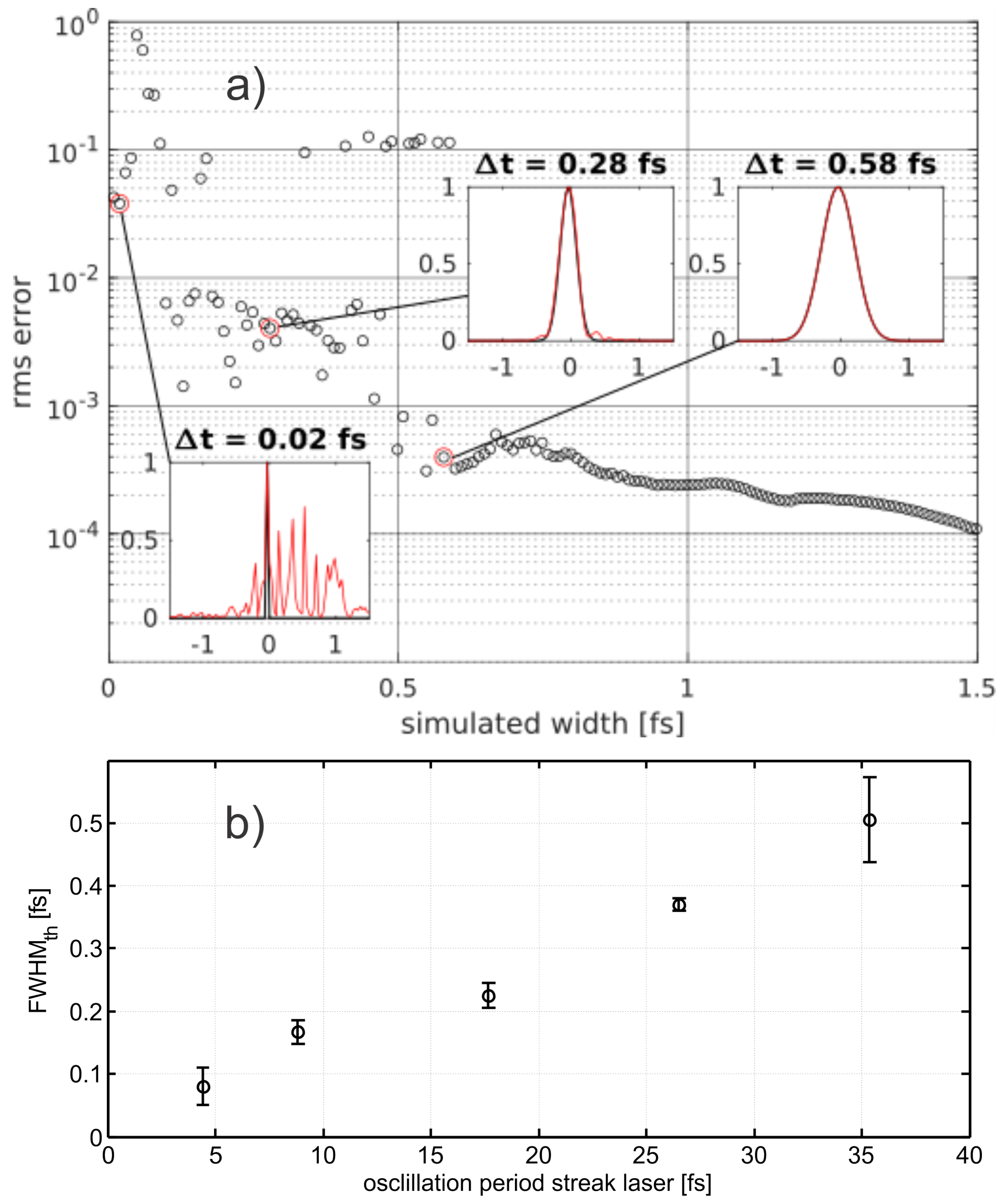
We began with a simple Gauss-shaped X-ray pulse of decreasing pulse duration in order to establish a lower bound for the feature sizes that could be reconstructed. Figure 1a shows the rms error for different pulse durations ranging from 0.01 fs to 1.5 fs. We identified three different regions, i.e., below 0.18 fs, between 0.18 fs and 0.5 fs and above. Below 0.18 fs, the reconstructed X-ray pulse contained mostly artifacts, as seen in the left-most inset, which shows the original (black curve) and the reconstructed (red curve) X-ray pulse. Between 0.18 fs and 0.5 fs, the main pulse was well reconstructed; however, we found reconstruction errors on both wings of the main pulse, as seen in the middle inset. Nevertheless, the quality of reconstruction was sufficiently high to estimate the pulse duration. For durations longer than 0.5 fs, the reconstructions were extremely good. As an example, the reconstruction of a 0.58 fs long Gaussian pulse is shown in the right inset. Further simulations indicated that the shortest pulse duration that could be reconstructed is linked to the oscillation period of the streak field, if all other parameters are kept constant. Figure 1b shows the FWHM of the shortest reliably reconstructed Gauss pulse versus the oscillation period of the streak laser. The error bars result from the uncertainty in determining the transition from a low (<${10}^{-3}$) to a high rms error (>${10}^{-1}$). These simulations suggest that a ratio of pulse duration over an oscillation period of less than 0.02 leads to erroneous reconstruction results.

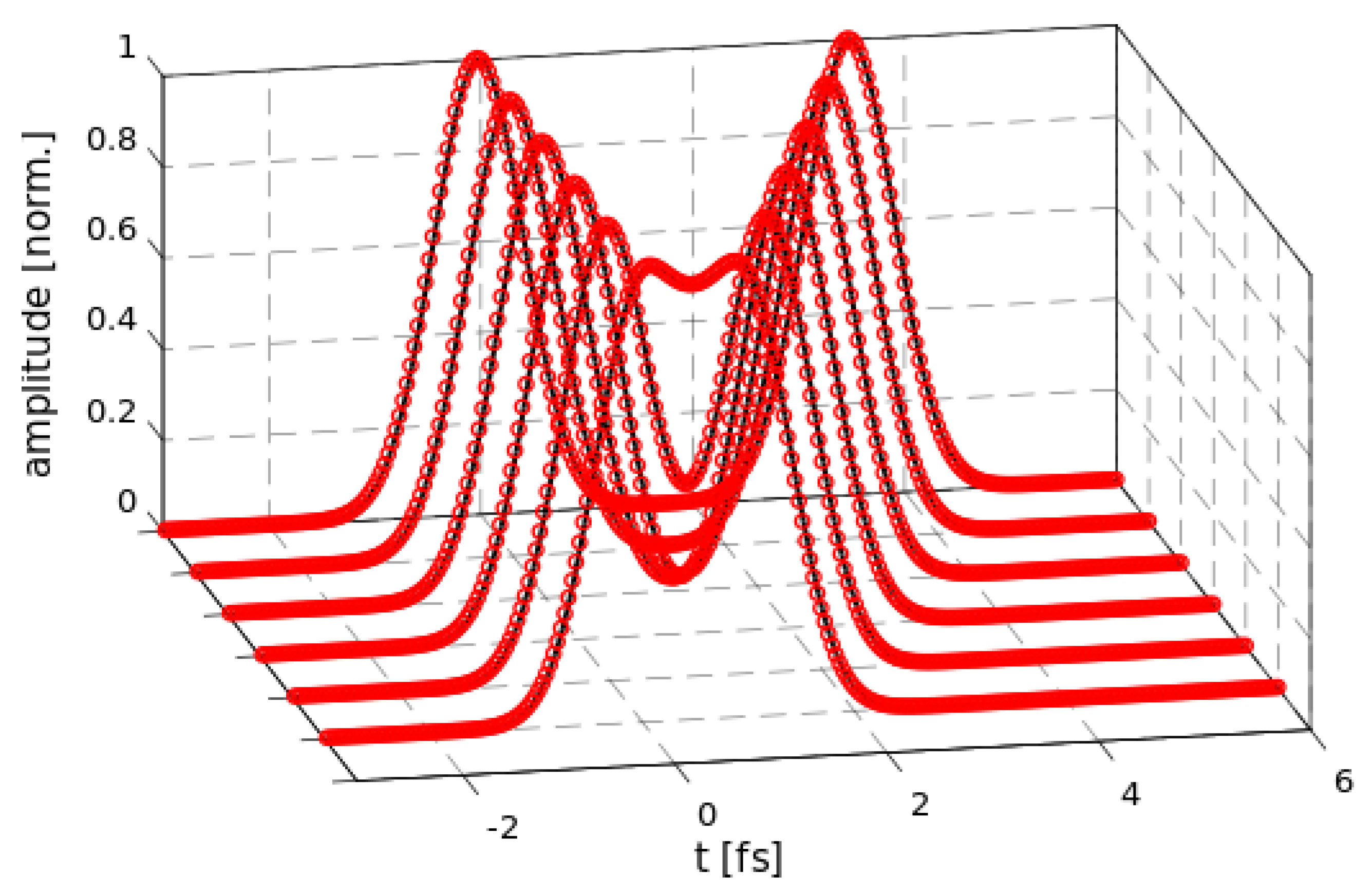
Next, we analyzed the reconstruction of X-ray waveforms consisting of two identical Gaussian pulses, each having a duration of 1 fs. Above, we have shown that single pulses with 1 fs duration are very well reconstructed. Such double pulses may be relevant for X-ray pump and X-ray probe experiments. One replica is fixed at the origin and the separation to the second replica is varied between 1 fs and 3.5 fs in steps of 0.5 fs. Figure 2 shows that in all cases, ptychography is able to yield an extremely accurate reconstruction result. The reconstruction is equally accurate for larger separations (not shown here).

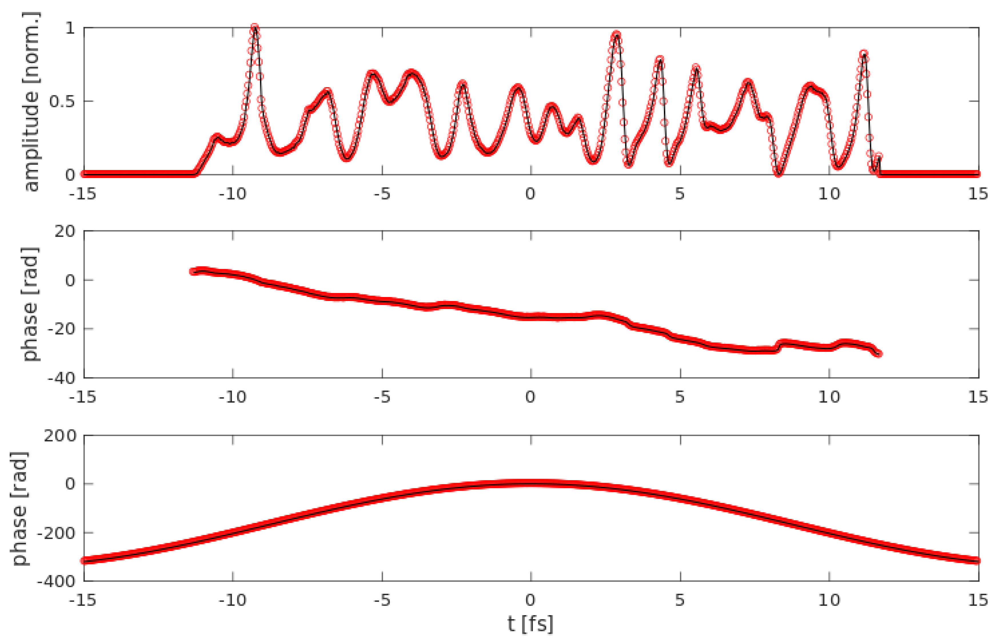
After exploring the temporal resolution limitations, we turned to more realistic X-ray pulses and used one of the SASE waveforms simulated for the Linac Coherent Light Source (LCLS). It consisted of about 20 randomly positioned SASE spikes with different amplitudes and durations between about 0.5 fs and 3 fs. The entire waveform was about 20 fs long and exhibited a minor global phase variation. Figure 3 shows the amplitude and phase (black curves) of this waveform. The red circles represent the reconstructed amplitude (top) and phase (middle), and we found a nearly perfect agreement between the two. We also show, for the sake of completeness, the original and reconstructed phases of the gate (bottom) and again, there is very good agreement. That is, ptychography is not only able to reconstruct simple well-behaved X-ray pulses but also complex waveforms, such as those generated by the amplification of noise in an unseeded free electron laser.

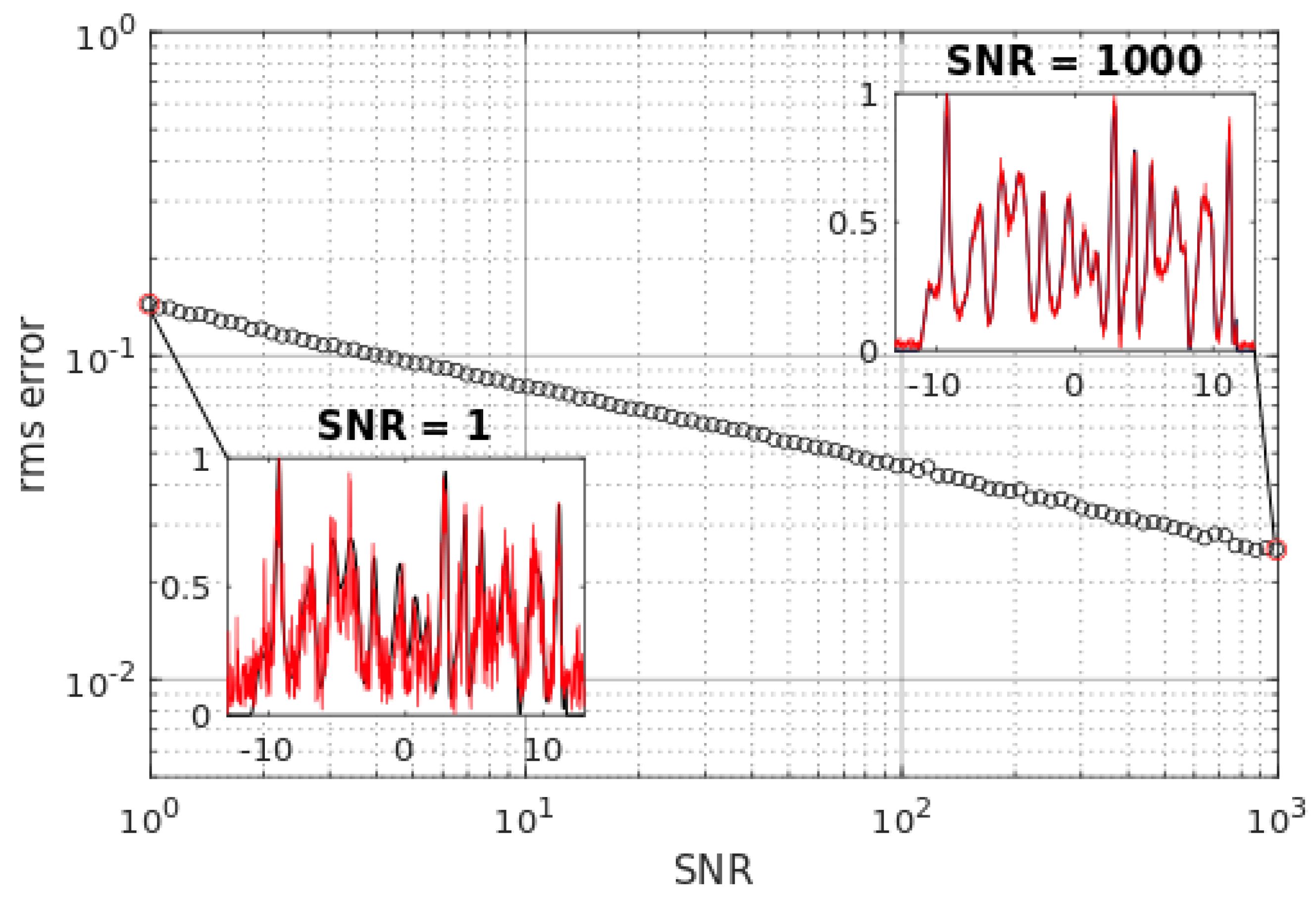
Since all measurements are subject to different noise contributions, we investigated the reconstruction error as a function of the signal-to-noise ratio (SNR). Figure 4 shows the rms versus SNR values ranging from 1 to 1000. As expected, the quality of reconstruction increased with SNR, but we found surprisingly good results even for low SNR values. The two insets show the reconstruction results for the two extreme cases, i.e., SNR = 1 and SNR = 1000. Even for SNR = 1, the reconstruction reproduced the most prominent features, albeit with substantial noise contribution. We also found that the rms error decreased with a slope of $-0.25$, which is reasonable because we added noise to the spectrogram and here, we expect a slope of $-0.5$ for pure statistical noise. The linear slope also indicates that the rms was dominated by the noise contribution and not by any additional reconstruction errors, especially for low SNR values.

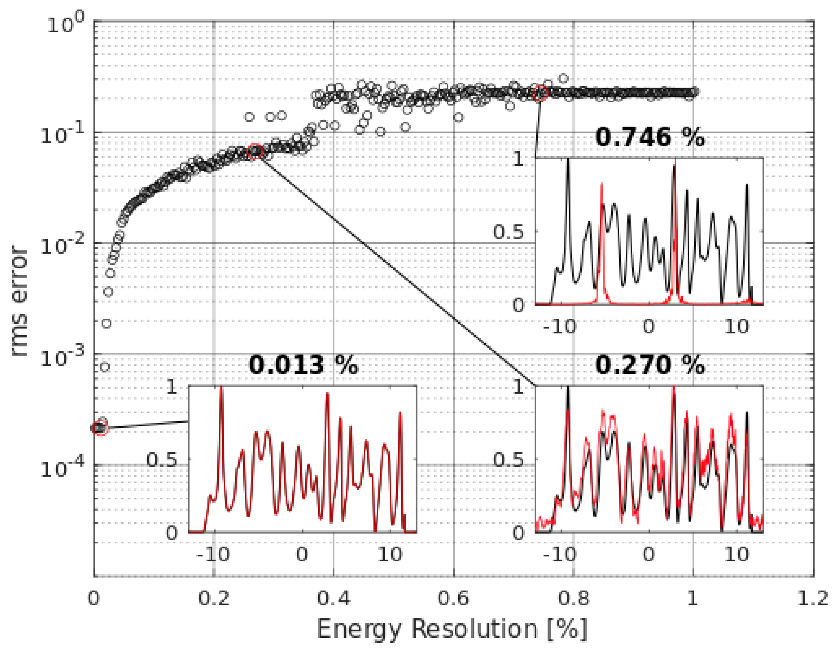
Another important aspect to consider is the influence of the finite energy resolution of the electron spectrometers used. In a recent experiment, electrons with a mean kinetic energy of approximately 310 eV were analyzed with electron spectrometers with an energy resolution of less than 1 eV [9]. That is, the relative energy resolution was in the order of ≤0.3%. Figure 5 shows the rms error for a relative energy resolution between 0% and 1%. For close to ideal energy resolutions, the reconstruction of the SASE waveform is very good, as shown in the left-most inset with the original waveform in black and the reconstructed waveform in red. With an increasing relative energy resolution, the error rapidly increased but we found good reconstruction results up to about 0.35% (see, for example, the lower right inset). For even worse energy resolutions, the error became almost constant at a level of rms ≈0.2, and the corresponding reconstruction results were no longer of reasonable quality.

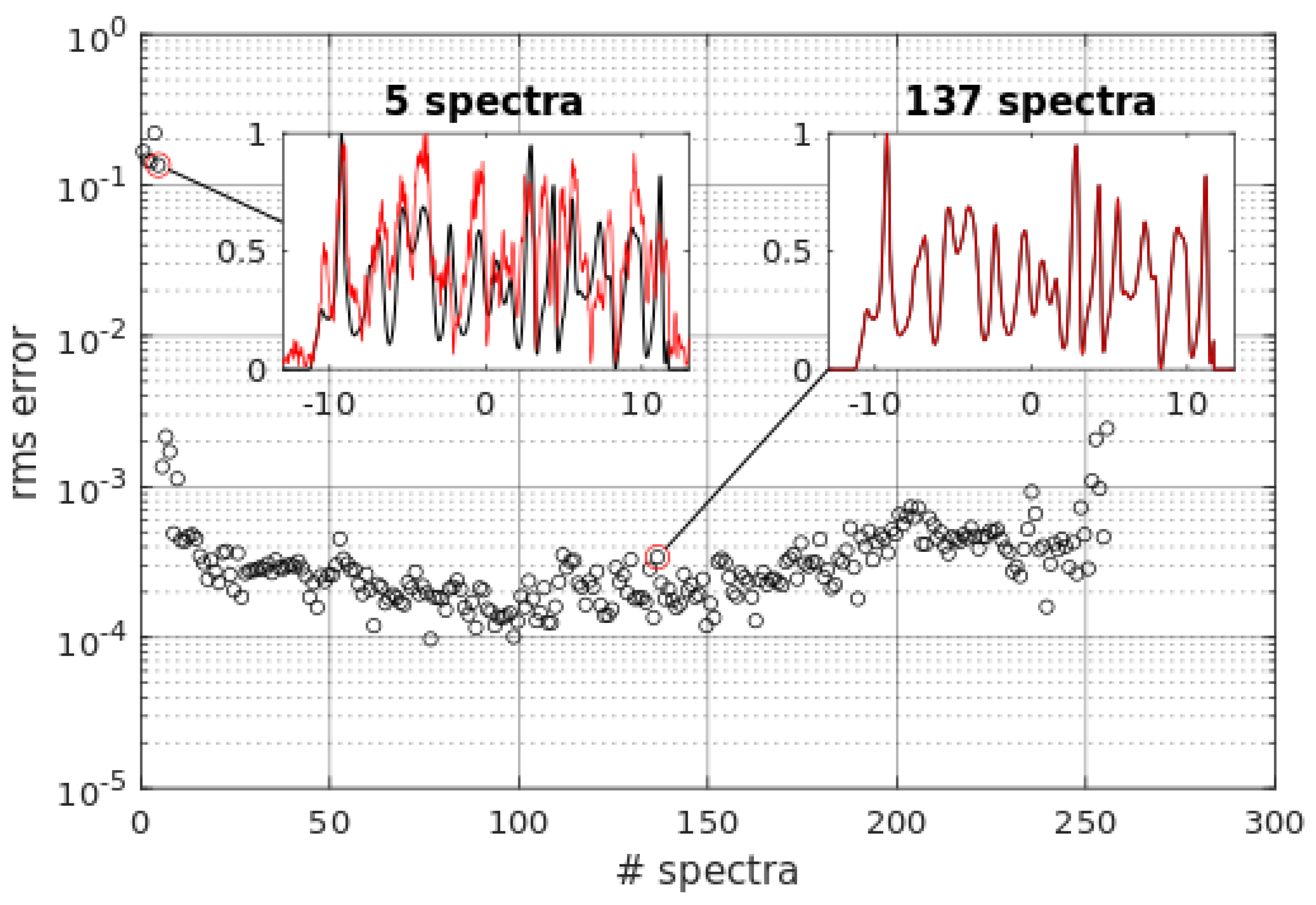
Finally, we investigated the number of spectra actually required for good reconstruction of the SASE waveform. Note that in angular streaking, the number of spectra is directly linked to the time delay increment, such that $N\delta \tau =2\pi /{\omega }_0$. That is, for $N=1$, we have $\delta \tau =35.4$ fs, and for $N=256$, the time delay increment is as small as $\delta \tau =0.14$ fs. Figure 6 shows the rms error starting with one spectrum to 256 spectra, which means that $\delta \tau$ simultaneously reduces from 35.4 fs to 0.14 fs. For less than five spectra, the rms error was prohibitively high and the reconstruction results were insufficient, as indicated in the left inset. However, 10 spectra and more yielded very good results (see, for example, the right inset). Consequently, recent experiments, which were conducted with 16 electron spectrometers arranged on a circle around the interaction volume [9], should have produced sufficient information for high quality reconstruction of complex SASE X-ray waveforms.

4. Summary and Outlook

In summary, we have shown that X-ray electron streaking experiments, typically resulting in a spectrogram with non-quadratic sampling, can be analyzed via ptychographic methods which reconstruct the amplitude and phase of complex X-ray pulses, such as those generated in an unseeded XFEL. Via dedicated simulations, we investigated the influences of noise, energy resolution and number of spectra recorded on the quality of reconstruction. We found that an SNR as low as five leads to very good results, the relative energy resolution of the electron spectrometer should be better than about 0.35%, and most surprisingly, ten spectra seems to be sufficient for a high quality reconstruction. The center wavelength of the streak laser and the timing jitter between the X-ray pulse and the streak laser define the shortest and the longest pulse duration that can be reconstructed. Finally, we would like to emphasize that good quality reconstruction can often be obtained after 10 to 100 iterations, making this method suitable for real-time shot-to-shot X-ray pulse monitors for most of todays machines with repetition rates of up to 100 Hz.

References

- Hoppe, W. Beugung im inhomogenen Primärstrahlwellenfeld. I. Prinzip einer Phasenmessung von Elektronenbeugungsinterferenzen. Acta Crystallogr. Sect. A 1969, 25, 495–501. [Google Scholar] [CrossRef]
- Spangenberg, D.; Neethling, P.; Rohwer, E.; Brügmann, M.H.; Feurer, T. Time-domain ptychography. Phys. Rev. A 2015, 91, 021803. [Google Scholar] [CrossRef]
- Spangenberg, D.; Rohwer, E.; Brügmann, M.H.; Feurer, T. Ptychographic ultrafast pulse reconstruction. Opt. Lett. 2015, 40, 1002–1005. [Google Scholar] [CrossRef] [PubMed]
- Lucchini, M.; Brügmann, M.H.; Ludwig, A.; Gallmann, L.; Keller, U.; Feurer, T. Ptychographic reconstruction of attosecond pulses. Opt. Express 2015, 23, 29502–29513. [Google Scholar] [CrossRef] [PubMed] [Green Version]
- Spangenberg, D.-M.; Brügmann, M.; Rohwer, E.; Feurer, T. All-optical implementation of a time-domain ptychographic pulse reconstruction setup. Appl. Opt. 2016, 55, 5008–5013. [Google Scholar] [CrossRef] [PubMed]
- Heidt, A.M.; Spangenberg, D.-M.; Brügmann, M.; Rohwer, E.G.; Feurer, T. Improved retrieval of complex supercontinuum pulses from xfrog traces using a ptychographic algorithm. Opt. Lett. 2016, 41, 4903–4906. [Google Scholar] [CrossRef] [PubMed]
- Grguras, I.; Maier, A.R.; Behrens, C.; Mazza, T.; Kelly, T.J.; Radcliffe, P.; Düsterer, S.; Kazansky, A.K.; Kabachnik, N.M.; Tschentscher, T.; et al. Ultrafast X-ray pulse characterization at free-electron lasers. Nat. Photonics 2012, 6, 852–857. [Google Scholar] [CrossRef]
- Eckle, P.; Smolarski, M.; Schlup, P.; Biegert, J.; Staudte, A.; Schöffler, M.; Muller, H.G.; Dörner, R.; Keller, U. Attosecond angular streaking. Nat. Phys. 2008, 4, 565–570. [Google Scholar] [CrossRef] [Green Version]
- Hartmann, N.; Hartmann, G.; Heider, R.; Wagner, M.S.; Ilchen, M.; Buck, J.; Lindahl, A.O.; Benko, C.; Grünert, J.; Krzywinski, J.; et al. Attosecond time–energy structure of X-ray free-electron laser pulses. Nat. Photonics 2018, 6, 852–857. [Google Scholar] [CrossRef]
- Huang, S.; Ding, Y.; Feng, Y.; Hemsing, E.; Huang, Z.; Krzywinski, J.; Lutman, A.A.; Marinelli, A.; Maxwell, T.J.; Zhu, D. Generating single-spike hard X-ray pulses with nonlinear bunch compression in free-electron lasers. Phys. Rev. Lett. 2017, 119, 154801. [Google Scholar] [CrossRef] [PubMed]
- Helml, W.; Maier, A.R.; Schweinberger, W.; Grguraš, I.; Radcliffe, P.; Doumy, G.; Roedig, C.; Gagnon, J.; Messerschmidt, M.; Schorb, S.; et al. Measuring the temporal structure of few-femtosecond free-electron laser X-ray pulses directly in the time domain. Nat. Photonics 2014, 8, 950–957. [Google Scholar] [CrossRef]
- Düsterer, S.; Radcliffe, P.; Bostedt, C.; Bozek, J.; Cavalieri, A.L.; Coffee, R.; Costello, J.T.; Cubaynes, D.; DiMauro, L.F.; et al. Femtosecond X-ray pulse length characterization at the linac coherent light source free-electron laser. New J. Phys. 2011, 13, 093024. [Google Scholar] [CrossRef]
- Gallmann, L.; Cirelli, C.; Keller, U. Attosecond science: Recent highlights and future trends. Ann. Rev. Phys. Chem. 2012, 63, 447–469. [Google Scholar] [CrossRef] [PubMed]
- Quéré, F.; Mairesse, Y.; Itatani, J. Temporal characterization of attosecond XUV fields. J. Mod. Opt. 2005, 52, 339–360. [Google Scholar] [CrossRef]
- Thibault, P.; Dierolf, M.; Bunk, O.; Menzel, A.; Pfeiffer, F. Probe retrieval in ptychographic coherent diffractive imaging. Ultramicroscopy 2009, 109, 338–343. [Google Scholar] [CrossRef] [PubMed]
- Maiden, A.M.; Rodenburg, J.M. An improved ptychographical phase retrieval algorithm for diffractive imaging. Ultramicroscopy 2009, 109, 1256–1262. [Google Scholar] [CrossRef] [PubMed]
- Boge, R.; Heuser, S.; Sabbar, M.; Lucchini, M.; Gallmann, L.; Cirelli, C.; Keller, U. Revealing the time-dependent polarization of ultrashort pulses with sub-cycle resolution. Opt. Express 2014, 22, 26967–26975. [Google Scholar] [CrossRef] [PubMed]
Figure 1.
(a) Rms error versus pulse duration of a Gauss-shaped X-ray pulse. The insets show the original (black curve) and the reconstructed (red curve) X-ray pulses for three different pulse durations, i.e., 0.02 fs, 0.28 fs and 0.58 fs. (b) Shortest reliably reconstructed pulse duration versus the streak field oscillation period.
Figure 2.
Ptychographic reconstruction of X-ray double pulses. Each pulse is 1 fs long and the time delay between the two replica increases from 1 fs to 3.5 fs in steps of 0.5 fs. In all cases, the reconstructed X-ray waveform (red circles) matches the original waveform (black curve) extremely well.
Figure 3.
Ptychographic reconstruction (red circles) of a simulated self-amplification of spontaneous emission (SASE) pulse (black curve). Top: amplitude, middle: phase and bottom: streak field.
Figure 4.
Ptychographic reconstruction of a simulated SASE waveform for a signal-to-noise ratio, increasing from 1 to 1000. The insets show the original (black curve) and the reconstructed (red curve) X-ray waveforms as functions of time for the two extreme cases, i.e., SNR = 1 and SNR = 1000.
Figure 5.
Ptychographic reconstruction of a simulated SASE waveform as a function of relative energy resolution. The insets show the original (black curve) and the reconstructed (red curve) X-ray waveforms as functions of time for %, 0.270% and 0.746%.
Figure 6.
Ptychographic reconstruction of a simulated SASE waveform as a function of the number of electron spectrometers. The insets show the original (black curve) and the reconstructed (red curve) X-ray waveforms as functions of time for five and for 137 spectra.
© 2018 by the authors. Licensee MDPI, Basel, Switzerland. This article is an open access article distributed under the terms and conditions of the Creative Commons Attribution (CC BY) license (http://creativecommons.org/licenses/by/4.0/).
Share and Cite
MDPI and ACS Style
Schweizer, T.; Brügmann, M.H.; Helml, W.; Hartmann, N.; Coffee, R.; Feurer, T. Attoclock Ptychography. Appl. Sci. 2018, 8, 1039. https://doi.org/10.3390/app8071039
AMA Style
Schweizer T, Brügmann MH, Helml W, Hartmann N, Coffee R, Feurer T. Attoclock Ptychography. Applied Sciences. 2018; 8(7):1039. https://doi.org/10.3390/app8071039
Chicago/Turabian StyleSchweizer, Tobias, Michael H. Brügmann, Wolfram Helml, Nick Hartmann, Ryan Coffee, and Thomas Feurer. 2018. "Attoclock Ptychography" Applied Sciences 8, no. 7: 1039. https://doi.org/10.3390/app8071039
Note that from the first issue of 2016, this journal uses article numbers instead of page numbers. See further details here.