Climate Change and Power Security: Power Load Prediction for Rural Electrical Microgrids Using Long Short Term Memory and Artificial Neural Networks

Abstract

Many of rural Alaskan communities operate their own, stand-alone electrical microgrids as there is no state-wide power distribution network. Although the fossil fuel-based power generators are the primary energy source in these isolated communities, an increasing number of microgrids have started to diversify their power supply by including renewable wind, hydro and photovoltaic energy sources. The integration and optimization of the multiple energy sources requires a design of a new power management system that can anticipate how much electricity will be drawn by the community and how much electricity will be generated from the renewable sources in order to control the fossil fuel-based generators to meet the community power demand. To address this problem, we designed a hybrid machine learning algorithm to predict community power draw as one module for the next generation microgrid power management system. The algorithm divides the task of a power load prediction into two sub-models: the first temporal model predicts the future weather conditions and the second model is trained to associate the predicted weather conditions with the community power demand. The results illustrate (1) the feasibility of building a machine learning algorithm that uses relatively small data for model training and validation, (2) the ability to predict the near-future community power load for the microgrids operating in the environments with highly dynamic weather conditions and (3) how the integration of multiple low quality future weather conditions produced high accuracy power load prediction.

1. Introduction

The rural communities of Alaska are often self-managed, electrical microgrid islands that primarily rely on diesel generators for power production. In recent years, an increasing number of rural communities have started to diversify their energy sources and integrate renewable energy sources into their microgrids. Many communities in Southeast Alaska rely on hydropower generation, the Southcentral communities use solar and wind power, while the subarctic communities of the North include geothermal, wind and in-river hydrokinetic power to offset the fossil fuel-based power generation (Note: Juneau, AK is not a microgrid and $100\%$ of the city’s power demand is hydropower generated).

The integration of the renewable sources of energy into microgrids is economically advantageous, but also presents risks and uncertainty. The frequency of extreme weather events is increasing which makes the long term predictions of the renewable power generation and the community’s power demand a challenge. In 2008, an unexpected increase in temperature and precipitation resulted in an avalanche that disrupted the water supply to the hydropower generators and resulted in the disruption of the electrical feed into Juneau. The event lasted six and a half weeks [1]. The isolation of many communities also adds to power insecurity as repairs and diesel fuel resupplies are often delayed due to bad weather.

The research goal is to build a forecast model that will predict the community power load for microgrid installations in highly variable weather environments, with the intent to integrate the model into the next generation electrical microgrid management system (EMMS). Existing research addresses the prediction of a community power load or a renewable power generation for the microgrid installations at locations with stable weather conditions in comparison to the common extreme weather changes of many Alaskan communities (Figure 1). Our results show that the power load prediction using a previously proposed, monolithic, recurrent neural network-based model would yield future power load predictions with only $10\%$ accuracy [2,3,4]. Limited research exists on how to model the electrical microgrid behavior for environments where the ambient temperature changes exceed $10{}^{\circ }$F in less than 20 min, multiple times a day, with sustained wind speeds of 60 mph and the wind gusts exceeding 100 mph possibly lasting several days, and sudden changes of the solar radiation dropping the power output from photovoltaic installations in excess of $80\%$ [5].

The novel contributions of this research are: (1) the design of a multistage, hybrid machine learning architecture that decouples the temporal predictions of a single model into two sub-models, the first one for the temporal predictions for future weather conditions and the second to associate the predicted future weather conditions with the expected power load and (2) the prediction of power load solely from the past weather observations without the models using the past power load data as their inputs. 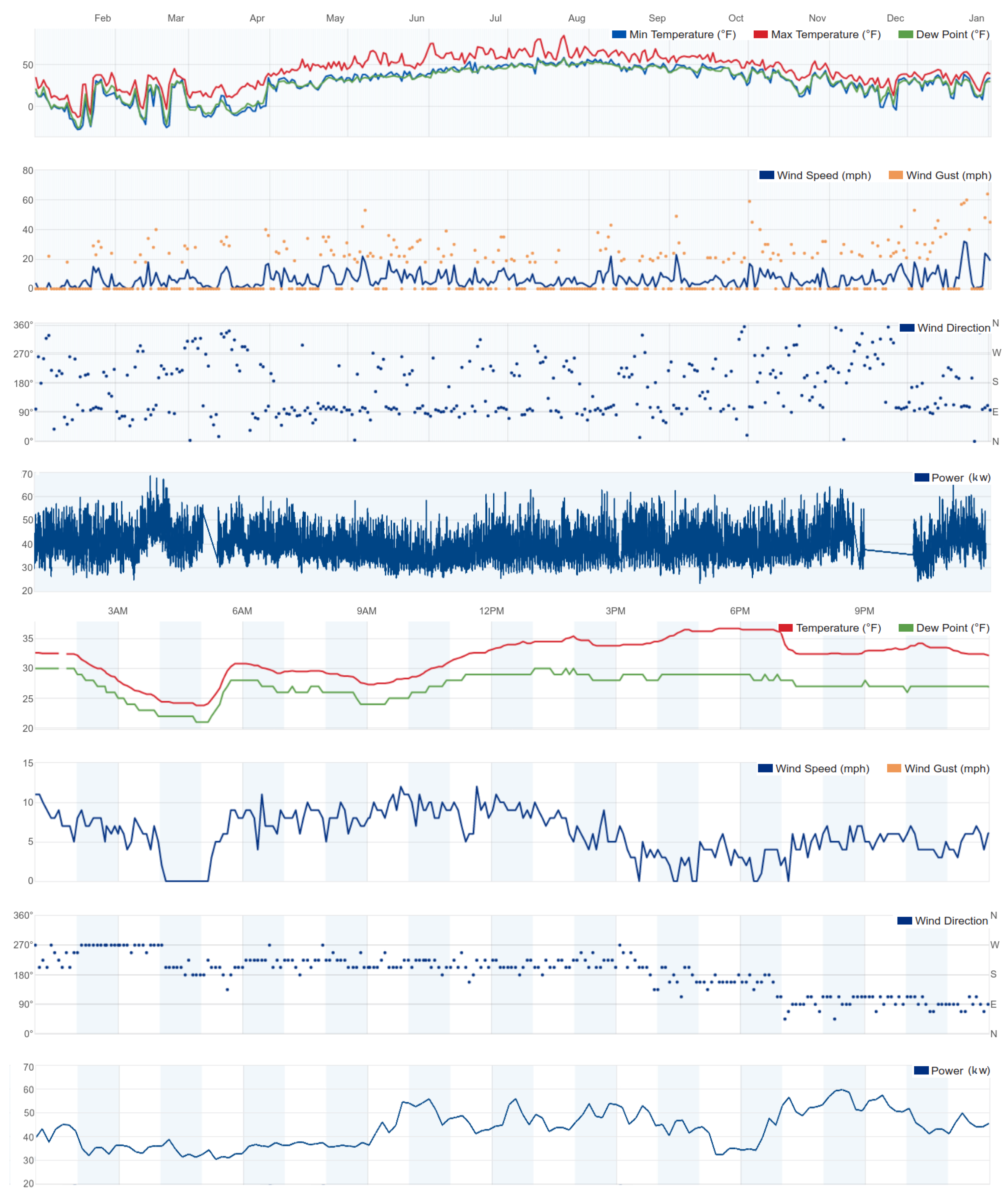Figure 1 shows the power load data is missing in mid-March and mid-November. The advantage of using a model ensemble that does not to rely on the past power load readings as their input is to make power predictions even for the days without the reported power load readings by using only the past weather conditions as the model inputs. The results show that the combined predictive accuracy of two individual sub-models is relatively low, but as an ensemble the framework will have high power load prediction accuracy. Finally, the proposed architecture illustrates the use of small data (less than one year) to successfully train and validate the individual sub-model.

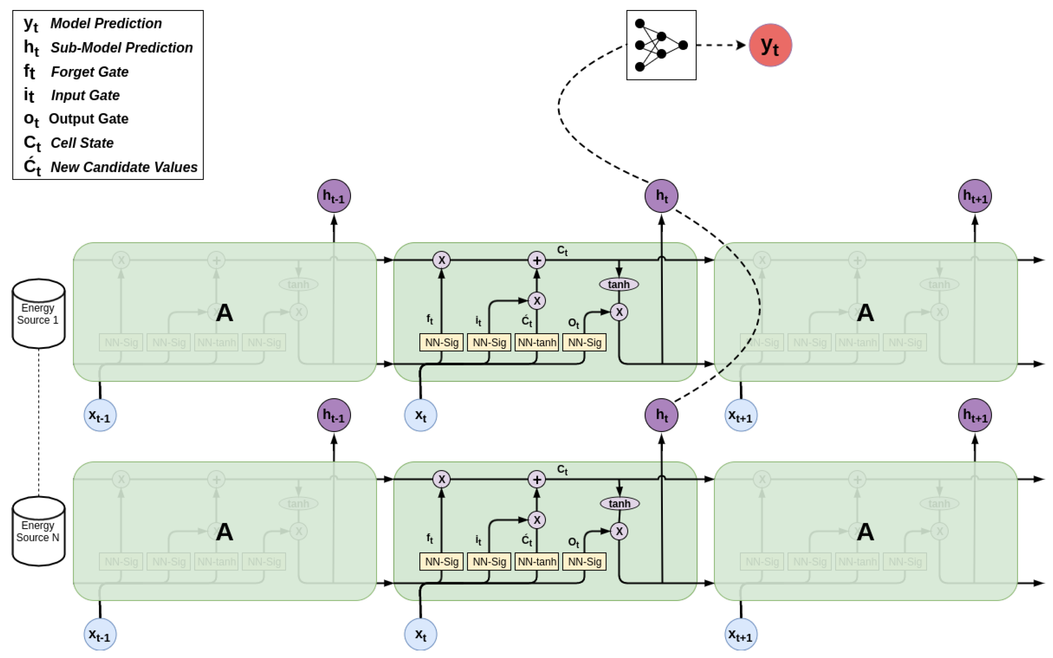
Figure 2 shows the design details of proposed hybrid machine learning architecture that consists of two sub-models. The advantage of dividing the prediction into two sub-models successfully mitigates the high volatility of the weather conditions and the associated uncertainty of predicting the community power load. The first temporal sub-model is trained to predict the near-future weather conditions given the past weather data (Figure 2 LSTM) while the second sub-model is trained to associate the historical weather conditions with the community power demand (Figure 2 ANN). The sub-models are validated individually on how accurately they predict the weather conditions and the power load respectively with reference to the recorded data. Finally, the power load prediction uses the past weather conditions as the inputs to the first temporal sub-model to produce the future predictions of weather conditions as its output. The outputs of the first sub-model are used as the inputs to the second sub-model to produce the power load predictions. The model ensemble accuracy is measured as a difference between the final predicted power load outputs from the second sub-model against the measured power load values. Since the first sub-model outputs the future weather conditions, thus making predictions in time, the second sub-model does not use time and only associates the future predicted weather with the power load.

The advantage of dividing the prediction into two sub-models include (1) the increase in accuracy in comparison to a single model with small data and (2) the ability to reuse the second sub-model to predict behavior of different electrical components of an EMMS. For example, Figure 2 shows the wind power model as an alternative reuse of the second sub-model to associate the predicted weather conditions with the wind power generation. The wind power generation predictions would use the same outputs of the first temporal sub-model but associate them with the wind power outputs in the second sub-model. In this case, the second sub-model is trained to associate the weather conditions with the wind power output. This design allows for an easy integration of any number of alternative energy generation sources or power load measured at different sub-stations as the EMMS prediction modules—where each EMMS module would correspond to one trained sub-model. This reuse of the second sub-model would not be possible if the model ensemble architecture would rely on the power readings as its inputs.

In the future, we plan to use the community power load and the renewable power generation models to optimize and control the fossil fuel-based power generators (either diesel or coal fired generators). The overall “super-model” architecture showed in Figure 2 can be used to implement the electrical microgrid management system which would allow for the long term planning of the fuel supplies, integration and optimization of a battery bank, and the intelligent scheduling of the community’s cyber-enabled, energy load dependent infrastructure to distribute the microgrid’s power load. One example is scheduling the operation of a micro water-treatment facility outside of peak demand times or when the EMMS generates excess power.

Figure 1 shows the measured power load behavior has low correlation to any one of the weather factors. Also, the power load does not have an easily discernible (asymptotic) trend of peaks during the morning and evening hours, or lower power consumption during the business hours, and does not have valleys during the commute periods. In addition to the ability to predict the community power load for the microgrids operating at locations with extreme weather conditions, we also address the question if the power load prediction using multiple weather factors will outperform the prediction accuracy using only the temperature measurements.

Although outside the scope of this project, the ability to accurately predict power generation from renewable energy sources in Northern latitudes is equally important and uncertain. The power generator manufacturers test their devices for a limited range of operating conditions which might not include extreme operating conditions that commonly occur in Alaska. As a result, the expected power curves often do not hold, so building machine learning models that associate the ambient environmental conditions with the power generation are needed. For example, the photovoltaic systems will produce electricity that exceeds the manufacturer’s maximum power generation simply because the photovoltaic cells installed in the Arctic are super cooled [6]. The energy production using the in-river hydroturbines is effected by sediment transport [7]. The icing on the wind-turbine blades creates added drag [8]. The concentration of the reflected ambient light from snow is often sufficient to produce electricity even during the low light conditions when no power generation is expected.

The Long Short Term Memory (LSTM) is a type of recurrent artificial neural network (RNN) model where the network’s inputs are processed in stages and the output of each stage (layer) is not only fed as the input to the next state, but the outputs are also reused as the inputs to the previous processing layers [9,10]. Additionally, the conventional node in a RNN is converted to a module that contains three gates. Each gate is a neural network with specific memory tasks, those being forget, input, and output. This architectural design creates directed loops in the information processing and captures the temporal dependency between consecutive instances of input data and thus implements the system’s memory. The architecture was first introduced in 1997 by Hochreiter et al. [9] and since the LSTMs were used in the electrical power domain to disaggregate the power signature of a single dominant appliance or a sub-circuit from the aggregate power signal [2], predict the wind power generation from the environmental conditions [3], and detect anomaly in sensor networks [11,12].

Xiaoyun et al. used the LSTM to predict wind power generation [3]. They used the principal component analysis (PCA) to narrow down the number of input variables from the original five variables that are included in the wind turbine output power equations to only two: wind velocity and wind direction. The cumulative contribution of these two parameters was $99.8\%$ of the overall data variance and the resulting LSTM predicted the wind power generation with an accuracy of $1.07\%$ normalized root mean squared error.

The long short term memory model for load forecasting with empirical mode decomposition was proposed by Zheng et al. [4]. The model forecasts the next hour peak energy load in the power grid as well as one day ahead load forecasting. The LSTM was trained on the grouping of days with similar environmental characteristics. The groupings were determined using K-means clustering algorithms with extreme gradient boosting [13]. The resulting prediction model had $\left(0.93,1.13\right)$ training error and $\left(1.01,1.34\right)$ mean absolute percentage error for the next day peak load prediction depending on the model’s configuration.

Amjady et al. designed a hybrid short term load forecast model to predict the power demand from load time series using neural networks and genetic algorithms-based models [14]. The forecast engine used a combination of a short term memory model and an evolutionary algorithm with the differential evolution algorithm as the performance optimizer for the forecaster. The prediction of the next day’s power generation achieved and average of $2.40$ weekly mean error on the four selected weeks between September and April.

An energy management system architecture for a microgrid control system was proposed by Saez et al. [15]. The fuzzy prediction interval models generalized the wind and solar power generation as well as the microgrid’s electrical load behaviors. The outputs of the prediction models were associated with the uncertainty values of the future predictions. The proposed model was designed as a sub-system to an EMMS. The test data was collected from a relatively stable microgrid installation in the Huatacondo microgrid in the Atacama Desert, Chile and both renewable energy generation and the loads were predicted with a mean absolute error of less than $1.1153$ kW.

Finally, a conventional heuristics-based energy management system was proposed by Kanchev et al. [16]. The accuracy of the proposed control and optimization strategy was assessed on a household photovoltaic array installation.

2. Methodology: Data Pre-Processing and Models

The data was collected from the Igiugig, AK (Latitude: $59.{3278}^{\circ }$ N, Longitude: $155.{8947}^{\circ }$ W) microgrid from 19 December 2013 to 17 December 2014. The weather conditions and the community power draw reports were temporally aligned and the reporting frequency was standardized to 10 min per reporting interval. The data collection was incomplete for the given time period, and the final data set had multiple periods of missing measurements for either the community power load, the weather conditions or both. Some of the missing weather data was filled in using the readings from other nearby weather stations that reported the environmental conditions on publicly available sites [17]. The incomplete instances in the final data-sets were disqualified and not used to train or assess the models.

The resulting data set associated each reported community power draw reading with the reported weather data vector that includes temperature, humidity, dew-point, wind speed, wind direction, wind gust speed, conditions, and events. The total number of complete instances is $38,661$ which is equivalent to approximately 268 days worth of usable data.

Each measurement category (feature) was pre-processed by feature scaling and normalization using $x_i^{{}^{\prime }}=\frac{x_i-x_{min}}{x_{max}-x_{min}}$ to map the values of each feature to the range $(0,1)$. The data points without the power draw value were omitted from the data set.

The data set was split into the training and validation subsets using $80\%/20\%$ ratio for the two sets. The training instances were used to build the models while the instances in the validation set were used to assess the models accuracy and were not used to train the models. Treating the training and validation subsets as mutually exclusive reduces the chance of the model over-training and a loss of generalization. The model training terminates if the model cost function is minimized to a desired accuracy or the maximum number of training epochs is reached (Figure 4).

The model training is performed in epochs and during each epoch multiple batches of data instances are selected from the training set. Training the temporal model to predict the weather conditions defines a data-point in the batch as the current weather condition and a discrete window of past and future measurements. The model uses the past measurements as the inputs to learn the prediction of the current and future weather conditions. The model to predict the power draw defines a batch data-points as a single measurement of community power-draw and the associate weather conditions at that time. The data-points in each batch were selected from the training set at random with uniform distributions with replacement.

2.1. Super-Model

Figure 2 shows the construction of two classes of models that divide the long term power load prediction into two stages. First, the temporal prediction models are trained to predict the future weather conditions given the past weather window. We implemented a Stacked Long Short Term Memory (LSTM) model to train the temporal weather prediction, and each weather factor was predicted using an individual LSTM model. The second model type associates the predicted future weather conditions with the community power load. We designed and trained the multilayer perceptron artificial neural network (ANN) to associate the weather conditions with the power demand.

The main reason for building a hybrid machine learning algorithm with the LSTM and ANN models is because of the size, continuity and diversity limitations of the available data-set used to train the models. The previous research suggests using a single LSTM architecture to train a power generation or power draw model [3,4]; we experimented with a single LSTM model that used the weather data as its inputs and predicted the future power load outputs, but the resulting prediction accuracy was less than $10\%$. The available data set is too small to train a single model—less than one year’s worth of data that had to be divided into the training and validation subsets. Also the data set is not continuous and several time periods were missing power load measurements and had to be omitted. Furthermore, the data had low diversity. We define the data diversity as the number of unique weather conditions and the associated power load measurements grouped into the similarity bins. Semantically, each bin represents a unique weather regime with associated power load. Ideally, the bins would have a uniform frequency distribution of the number of data instances in each bin. On the contrary, the bin frequency distribution was skewed and with some bins with high frequency count and several bins with a few (less than 5) instances. Each bin had to be further split into the training and validation subsets. The compound effect of data scarcity and the lack of diversity resulted in low power prediction accuracy model.

2.2. Long Short Term Memory Model

Using the TensorFlow libraries (https://www.tensorflow.org/), we designed a stacked LSTM that allows for a configuration of multiple parameters including: the past history window, configuring how long of the past history should be used to predict current and future weather conditions, number of the gated recurrent units (GRU) in each hidden layer of the LSTM, number of stacked layers to determine the memory length, and how far into the future the network should forecast the grid behavior (number of output variables) [18,19]. The cost function minimization is defined as the mean between each of the predicted time-bound variables, while the Adam optimizer orchestrates the learning (Adam: an extension of a gradient descent optimization that uses the adaptive moment estimator) [20]. Furthermore, the stacked LSTM consists of layers of GRUs, and as the network’s depth increases (by increasing the number of hidden layers), so does the system’s memory of the past used to make the future predictions. The learning rate is reduced over time, described as:

while (step*self.batch_size<self.training_iters) and
(testing_loss_value > target_loss):
current_learning_rate = self.learning_rate
current_learning_rate *= 0.1 **
((step * self.batch_size) * self.training_iter_step_down_every)

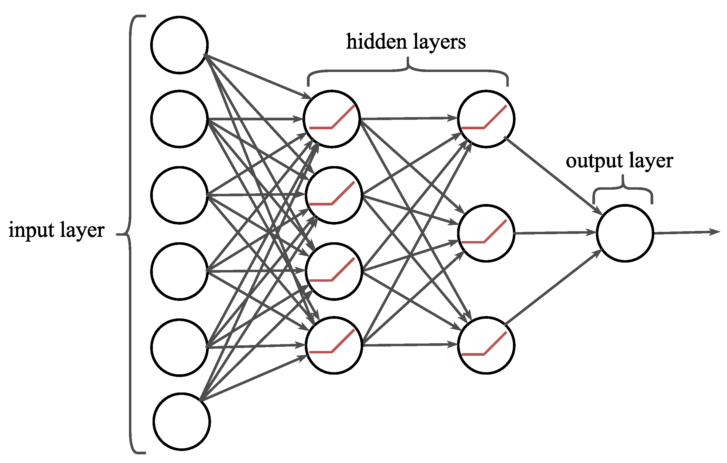
Figure 3 shows the illustration LSTM with three hidden layers of memory cells controlled at time t by the input $x_t$, the sate $c_t$ and the outputs parameters $o_t$ and $c_t$. The input gate transform $i_t$ is defined as $i_t=g(W_{xi}{x}_t+W_{hi}{s}_{t-1}+b_i)$, the forget gate $f_t$ where $f_t=g(W_{xf}{x}_t+W_{hf}{s}_{t-1}+b_f)$, the output $o_t=g(W_{xo}{x}_t+W_{ho}{s}_{t-1}+b_o)$, the input transform ${c^{\prime }}_{int}=tanh(W_{xc}{x}_t+W_{hc}{s}_{t-1}+b_{cin})$, the cell’s internal memory is updated by $c_t$ = $f_c\ast c_{t-1}\ast i_t\ast c_{int}$, and the state is updated using $s_t=o_t\ast tanh\left(c_t\right)$. The activation function g is implemented as a sigmoid function and the weights W are evolved by training the model on data [13]. Our LSTM instance used three hidden layers with 300 memory cells in each layer. The model’s weights were updated using a batch size of 100 instances.

The LSTM parameters were empirically tuned with the following parameter values: the learning rate = $2.5\times {10}^{-5}$, the past history windows length = 30, the number of output cells = 5, the number or GRU = 200, the number of hidden layers = 8, the criteria to terminate the model training is either the error loss = $1.0\times {10}^{-7}$ or a maximum of training epochs = $1.0\times {10}^6$, and the LSTM had 4 outputs where each output predicted the weather conditions for 10 min into the future (the total of 40 min).

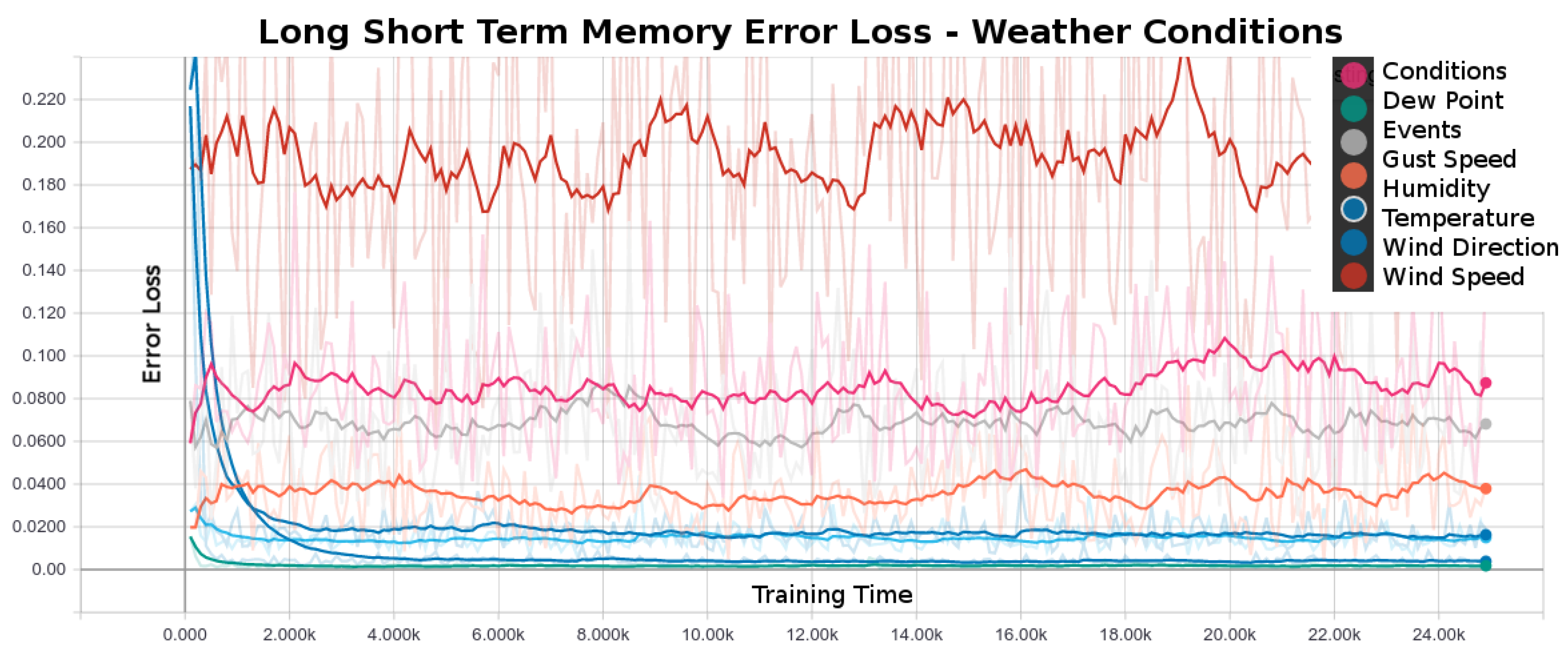
Each plot series in Figure 4 shows the error loss during the LSTM training, in other words, the plot lines show how well each the LSTM generalized the weather condition training data. The LSTMs trained on the data for wind direction, conditions, events and the wind gust speeds were the hardest to generalize and resulted in LSTMs with poor quality of predictions (top four plot series in Figure 4 respectively). A poor quality of LSTM models could be a result of an inconsistency or subjective judgment of a human observer in the categorization of the weather data and the subsequent labeling of the weather conditions. The labeled data series are the overall weather conditions and the weather events. The models failed to generalize the wind gust direction or the wind gust speed weather conditions because the weather data was collected from a limited geographical area and the microclimate data does not captivate information from a larger geographical region that would allow to predict the local “anomaly” events. The humidity, wind speed, temperature and dew point LSTMs had the most significant error loss and predicted the current and future weather conditions most accurately. On several independently executed experiments with a random seed, we observed that the training of the temperature and the dew point LSTM models terminated before the maximum number of training epochs was reached because the models reached the desired error loss threshold.

2.3. Artificial Neural Network

The ANN makes the discrete power predictions without the knowledge of time, since the LSTMs already do the temporal predictions of the weather conditions (Figure 5). The ANN uses the LSTMs’ outputs and predicts what would the community power load be for given weather conditions. The only difference between the ANN’s predictions of the short or the long-term power load is in the weather condition predictions it uses as its inputs—for the short term predictions, the ANN uses the LSTMs’ short term weather predictions and for the long term predictions it uses the LSTMs’ predictions farther out in time.

The ANN is trained using the current weather conditions to predict the community power load for the current conditions. Once trained, the ANN’s inputs are the LSTM outputs of the predicted future weather predictions. The network’s inputs are the outputs of multiple LSTMs, where each temporal model predicts the future weather condition of a single weather factor. This ANN configuration integrates the predictions of multiple weather features.

The ANN’s cost function is the mean squared error (MSE) between the expected power load prediction (network’s output) and the actual power load recorded in the collected data. The network uses the error back-propagation to adjust its weights. The weights were updated using an Adam optimizer–an extended version of the gradient descent optimization algorithm [20]. The network parameters were manually tuned and the final parameter values that produced the highest accuracy of power prediction used: the number of hidden layers = 4, the number of neurons in each hidden layer = $300,500,500,300$, the number of instances in each batch = 500, and the number of epochs = 200. Recall that the batch instance was defined as a weather feature vector and a power load readout. Each neuron in the hidden layer used the rectified linear unit (ReLU) activation function [21].

3. Results and Discussion

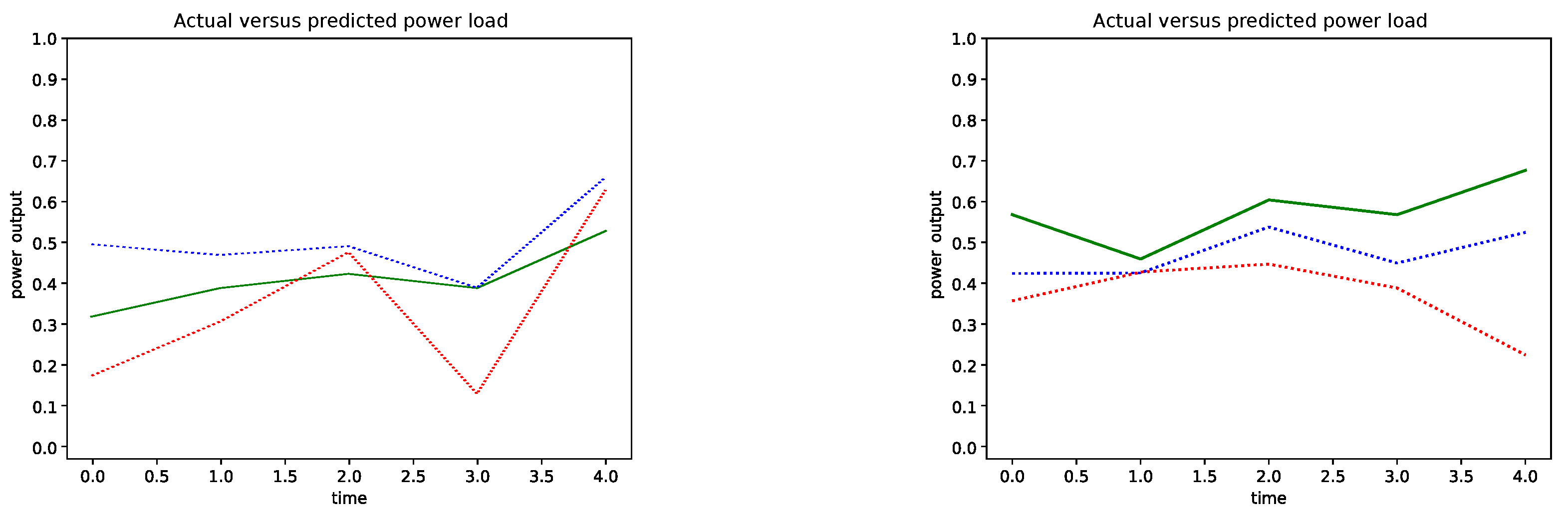
Figure 6 shows two examples of the community power load forecast from the start time to 40 min into the future. The blue plot line is the power prediction output of the ANN that used the LSTM’s predictions of the future weather conditions. The red plot line is the power prediction output of the ANN that used the measured (actual) weather conditions, which illustrates the ability of the ANN to forecast the power load having the perfect weather measurements but no knowledge of the past weather conditions. The error between the measured power load readings (green) and the predictions (blue) are much smaller then the error between the measured power load (green) and the ANN’s discrete power load predictions using the perfect weather data. The power predictions that used the LSTM’s future weather forecast resulted in the overall smaller error which is an evidence that the temporal model generalized the weather trends in the past weather window to produce higher accurate power load predictions. In contrast, the ANN makes power load predictions with greater error even if it has the perfect weather measurements which do not take into the account the past weather conditions. In other words, the ANN error to predict the power load was consumed by the LSTM memory of the past weather which produced a smoothing effect for the ANN predictions.

The overall prediction trends in Figure 6 illustrate the instability of the power load predictions made further out into the future. The instability in the left sample is visible as a non-monotonic prediction trend and a high variance of the prediction 30 min into the future. The sample prediction output on the right shows the instability by the divergence of the predictions from the measured power load, especially noticeable for the predictions 30 and 40 min into the future.

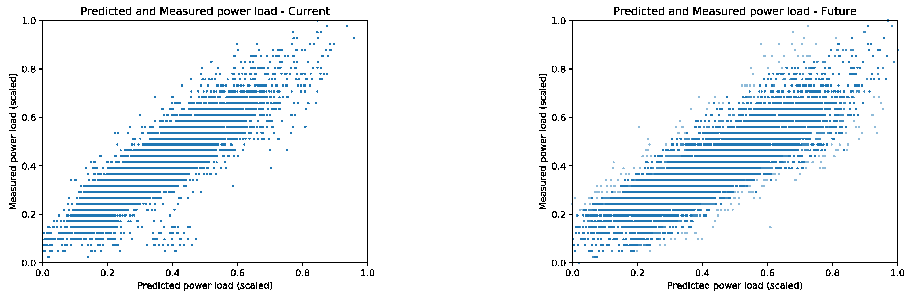
The cumulative assessment of the predictions using the validation set is presented as a correlation plot between the actual power load measurements and the outputs of the ANN that used the LSTM weather predictions to predict the power load. Figure 7 shows the future predictions on the x-axis and the measured power load on the y-axis. The points closest to the diagonal are near perfect predictions, while the points below the diagonal are higher predictions than measured and the lower predictions for the measured power load are above the diagonal.

Figure 7 (left) shows the current power load predictions using current weather conditions without any knowledge of the past weather. The results are reported after 200 training epochs on the validation data. The plot does not show any future predictions, it shows how well the ANN generalized the association of the weather conditions and the power load. Each point is a prediction of a current power load given the measured weather conditions. Model’s overall error is to produce lower power load predictions in comparison to the measured behavior which is seen as the predictions’ trend-line slope greater than ${45}^{\circ }$ .

Figure 7 (right) shows the future power load predictions using the future weather conditions predicted by the LSTM’s outputs. Again, the ideal power load predictions are the prediction points on the plot’s diagonal. The future power load predictions have higher variance from the diagonal which shows the future power load prediction error. The point’s color intensity represents how far into the future the prediction is made; the current predictions are the darkest but as the predictions are made farther out in time the point’s color gets lighter. The power load predictions made further out into the future have higher error from the reported power load. Interestingly enough, the overall slope of the ANN predictions that use the LSTM future weather predictions is closer to the diagonal (right) then the ANN predictions of the current power load predictions (left) that used the actual weather measurements. This observation is an evidence that the ensemble of a temporal and an associative model together produce power load predictions with less error that are closer to the measured trends.

The reported results in Figure 7 used all weather features available without performing Principal Component Analysis to determine which weather variable captures the variance in the measured power load. The forecasting accuracy was measured using the normalized mean squared error $MSE=\frac{1}{N}\sum _{i=1}^N{(\widehat{y}\left(i\right)-y\left(i\right))}^2$ for the number of validation samples N, where $\widehat{y}\left(i\right)$ is the LSTM’s output on the data point i given the past weather window and the $y\left(i\right)$ is the expected (measured) value on the data point i. The verification set size was $20\%$ (7731 possible measurements) of the entire data set.

The validation results for the ANN trained to associate the weather conditions and the power load showed in Figure 7 had the MSE = $3.61\times {10}^{-3}$ to predict the current power load (left) and the MSE = $3.65\times {10}^{-3}$ to predict the future power load for 40 min into the future (right).

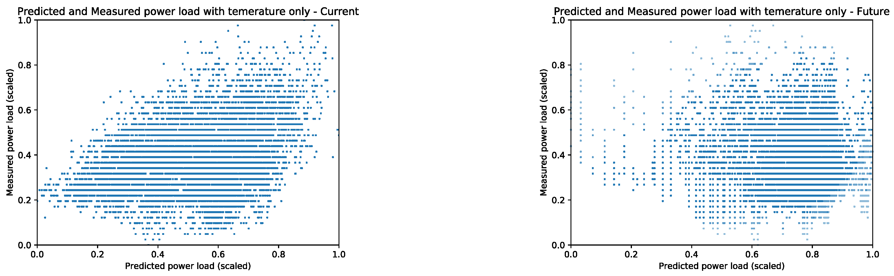
How much power load prediction depends solely on the temperature is showed in the results Figure 8. Instead of using all available weather features, we trained the ANN to only use the temperature to predict the current power load (left) and used the LSTM’s predictions for the next 40 min to forecast the power load. The results indicate that the power load is dependent on other weather factors than just the temperature. The results in Figure 8 show this by an order of magnitude higher MSE than the power predictions using all available weather features (Figure 7). The MSE in Figure 8 had the MSE = $1.20\times {10}^{-2}$ for the current power load predictions and MSE = $1.66\times {10}^{-2}$ to predict the future power load conditions.

Furthermore, Figure 8 shows that using only the temperature had disproportionally lower quality of the power load predictions for the reported power load values less than $0.5$ for both the current and future predictions. The results in Figure 7 used the full weather feature vector had high generalization across the range of possible power load values. In summary, the presented results show that including additional weather conditions to the feature set will result in more accurate forecasts.

The final results set in Figure 9 show the ability of the individual LSTM models to generalize the weather condition trends to predict the current and the future weather conditions. The sample results in the left column had overall lower generalization error loss, while the weather conditions in the right column were predicted more accurately with higher error loss (see Figure 4 for details).

The analysis of the LSTM prediction quality by a standalone model are misleading, because (1) the power load prediction is made in conjunction with the ANN, (2) the MSE values of the LSTM models measure the absolute value between the measured and predicted weather conditions rather than how accurate is the predicted weather trend for the power load prediction and (3) the ANN integrates the outputs of multiple weakly predicted weather futures into the final power load prediction.

4. Conclusions

We presented a hybrid machine learning approach to predict the community power load dynamics. Although the scope of presented work is to model one aspect of the energy management system, the hybrid super-model can be expanded to contain the power generation models and the diesel generator control system. Each of the renewable models would generalize the behavior of a single renewable energy source such as a photovoltaic, hydrodynamic, or wind-turbine power generators. Modeling behavior of the renewable energy sources would use the same modeling approach as the community power load: the LSTM would predict the future weather conditions and the behavior of each renewable energy source would be modeled by an individual ANN. Each ANN would bind predicted future weather conditions and the power production of a renewable energy source.

The advantage of designing multiple models to predict the electrical microgrid behavior is in the transparency of the resulting electrical microgrid management systems. With dedicated ANN models, each constituent component of the control system can be individually examined, optimized or controlled. The prediction mechanism is divided into the temporal weather condition LSTM model and the ANN power model which allows for the reuse of the LSTM by multiple power models. In other words, if new weather features or additional weather readings become available, only the LSTM model has to be retrained to increase the prediction accuracy of the future weather conditions, while the power models can remain unchanged.

We illustrated how a relatively small data set can be generalized using hybrid model design that breaks up the prediction task into two submodels. Unlike the previous research, the proposed machine learning algorithm does not group the similar weather days into clusters to train the model, instead we define past and future weather windows for the current condition readings and use this data as a discrete data point to train the LSTM. Treating each reading as a discrete data point allows the algorithm to predict future weather conditions that include dynamic and extreme weather events.

Using a single LSTM that would associate the current weather conditions with the community power load forecast yields low accuracy of less than $10\%$. The main reason for low accuracy is the fact that the model was expected to perform a two step inference of predicting what the weather would be in the near future and associating the weather prediction with the power load. By splitting a single LSTM model into two submodels we minimized the prediction error in each submodel. We hypothesize that a single LSTM model might achieve high prediction accuracy using a sufficiently large data set to train a single LSTM. The available data for the presented work had less than one year of power load readings with a limited number of unique weather events (discretized and binned). For example, the data set contains only one weather event of extremely low temperature below $-35{}^{\circ }$F. To improve the model accuracy, the training and the validation sets have to include multiple events in each weather regime category (conditions bin).

Using a small data set also limited which additional input features were used to construct the model. For example, the temporal LSTM does not use the day of the week or the time of the day, because the model training and validation required multiple instances of similar weather vectors. Given the available data, many of the weather regime bins had a low number of weather vectors. Including the day and time as additional input features would further decrease the frequency counts in each weather regime bin. In other words, the power load prediction for weather vector with $32{}^{\circ }$F, with no wind, and low humidity will be different if this weather regime occurs at midnight when people keep their house temperature low, or at mid-day on Saturday, or at mid-day during the work day. (In many rural communities in Alaska, approximately $80\%$ of the electrical power is used to heat the residential houses). When multiple years of data are available and each weather regime bin will have multiple weather vectors, the model training and validation can include the day and time of the week as the additional input features to increase the overall power load prediction accuracy.

To build a high fidelity electrical microgrid management system that will dynamically throttle the fossil fuel-based generators to meet the predicted community power load, we will have to address the issue of the temporal delay of the power load changes with respect to the measured changes in the weather conditions. For example, if a new weather system starts effecting local climate, the community will not change their power demand immediately and the changes to the power load will lag in time. To address this phenomena, we will investigate the relationship between the length of the past weather windows and the temporal delay on the accuracy of the future power load prediction. We will aim for a single, deep (large number of hidden layers) LSTM that uses long history window to be able to predict power draw into more distant future with high accuracy.

The last factor that should improve the model’s accuracy to predict the power load forecast is to include additional features in addition to the environmental conditions. These features should describe the social dimension of the community dynamics and include information such as which day of the week the measurement is associated with, if the school is in session, if the time of the day is associated with the working hours, community event calendar etc.