Multiwavelength Absolute Phase Retrieval from Noisy Diffractive Patterns: Wavelength Multiplexing Algorithm


1
Laboratory of Signal Processing, Technology University of Tampere, 33720 Tampere, Finland
2
Department of Photonics and Optical Information Technology, ITMO University, 197101 St. Petersburg, Russia
*
Author to whom correspondence should be addressed.
Appl. Sci. 2018, 8(5), 719; https://doi.org/10.3390/app8050719
Submission received: 26 March 2018
/
Revised: 29 April 2018
/
Accepted: 30 April 2018
/
Published: 4 May 2018
(This article belongs to the Special Issue Applications of Digital Holographic Microscopy)
Abstract
:We study the problem of multiwavelength absolute phase retrieval from noisy diffraction patterns. The system is lensless with multiwavelength coherent input light beams and random phase masks applied for wavefront modulation. The light beams are formed by light sources radiating all wavelengths simultaneously. A sensor equipped by a Color Filter Array (CFA) is used for spectral measurement registration. The developed algorithm targeted on optimal phase retrieval from noisy observations is based on maximum likelihood technique. The algorithm is specified for Poissonian and Gaussian noise distributions. One of the key elements of the algorithm is an original sparse modeling of the multiwavelength complex-valued wavefronts based on the complex-domain block-matching 3D filtering. Presented numerical experiments are restricted to noisy Poissonian observations. They demonstrate that the developed algorithm leads to effective solutions explicitly using the sparsity for noise suppression and enabling accurate reconstruction of absolute phase of high-dynamic range.
1. Introduction
Reconstruction of a wavefront phase is on demand in holography [1,2], interferometry [3], holographic tomography [4,5] and is of general interest due to important practical applications in such areas as biomedicine (for instance for studies of living cells [6,7]), 3D-imaging [8], micromachining [9], etc. There are two different approaches for extraction of spatial phase information. The first, which is associated with the holography, implies recording interference patterns of object and reference waves, while the second approach involves only sets of coherent diffraction patterns of object without reference waves. In these intensity measurements the phase information of the registered wavefields is eliminated, and then reconstructed by means of numerical iterative algorithms. The latter problem is well known as the phase retrieval, where “phase” emphasizes that the missing phase defines the principal difficulty of the problem and its difference with respect to holography.
The first phase retrieval algorithm was introduced by R. Gerchberg and W. Saxton [10]. They used squared roots of intensities measured in image plane to replace amplitudes calculated in iterations. Important update was developed by J. Fienup [11], who introduced constrains for the iterative process by the amplitude distribution in Fourier plane, namely, a nonnegativity of the reconstructed image and energy concentration in a certain area. A dataset of recorded intensity patterns which is characterized by diversity of one or several parameters of the optical setup is a crucial moment of the phase retrieval problems. Defocusing and phase modulation are known as effective instruments in order to achieve the measurement diversity sufficient for reliable phase reconstruction (e.g., [12,13,14,15]). Various types of diffraction optical elements can be used for design of phase imaging systems [16]. The review and analysis of this type of the systems as well as further developments of the algorithms can be found in [17].
There are various optimization formulations of conventional Gerchberg-Saxton (GS) algorithm [18,19,20]. Contrary to the intuitively clear heuristic of the GS algorithm, the variational approaches have a stronger mathematical background including image formation modeling, formulation of the objective function (criterion) and finally going to numerical techniques solving corresponding optimization problems. The recent overview [21] is concentrated on the algorithms for the phase retrieval with the Fourier transform measurements and applications in optics. The constrains sufficient for uniqueness of the solution are presented in detail. The fundamental progress for the methods based on the convex matrix optimization is announced in [22], where the novel algorithm ”Sketchy Decisions” is presented. This algorithm is effective for high dimensions typical for the phase-lifting methods and is supported by the mathematical analysis and the convergence proof. The Wirtinger flow (WF) and truncated Wirtinger flow (TWF) algorithms presented in [23,24] are iterative complex-domain gradient descent methods applied to Gaussian and Poissonian likelihood criteria, respectively
The techniques based on the proximity operators developed in [25,26] provide a regularized optimization of the maximum likelihood criteria also for both Gaussian and Poissonian observations. The sparsity based techniques is a hot topic in phase retrieval (e.g., [27]). A sparse dictionary learning for phase retrieval is demonstrated in [28]. The transform domain phase and amplitude sparsity for phase imaging is developed in [29,30,31]. For the phase retrieval these techniques are applied in [32,33,34].
In recent years, there has been an increase in demand for multispectral imaging. Multispectral information by recording object waves with multiple wavelengths that are irradiated from multiwavelength light sources helps to analyze and recognize objects, to clarify color and tissue distributions and dramatically improves the quality of imaging. Multiwavelength digital holography has an enhanced ability for 3D wide-range shape measurements by using multiwavelength phase unwrapping, due to the recording of multiwavelength quantitative phase information. The multiwavelength is an effective instrument enabling good phase and data diversity in phase retrieval.
The multiwavelength absolute phase imaging is much less studied as compared with the standard single-wavelength formulation. These works by the principle of measurements can be separated in two groups. In interferometry and holography scenarios the reference beams are applied to reveal the phase information, e.g., [35,36,37,38,39,40]. After that, the phase unwrapping algorithms for 2D images are applied. Recently, the phase unwrapping with simultaneous processing of multiwavelength complex-exponent observations have been developed based on the maximum likelihood techniques [41,42].
Another group of the multiwavelength absolute phase imaging techniques uses as measurements amplitudes or intensities of coherent diffraction patterns of an object without reference waves. In these intensity measurements the phase information is missing. These formulations are from the class of the multiwavelength phase retrieval problems, e.g., [43,44,45,46,47,48].
The Chinese Remainder Theorems, existing in many modifications, provide methods for absolute phase reconstruction from multiwavelength data for noiseless data [49]. The reformulation of these mathematically strong approaches for more practical scenarios with noisy data and for robust estimation leads to the techniques similar to various forms of maximum likelihood [50,51].
In this paper we study the problem of multiwavelength absolute phase retrieval from noisy object diffraction patterns with no reference beams. The system is lensless with multiwavelength coherent input light beams and random phase masks applied for wavefront modulation. The light beams are formed by light sources radiating all wavelengths simultaneously and a Complementary Metal Oxide Semiconductor (CMOS) sensor equipped by a Color Filter Array (CFA) is used for spectral measurement registration. The developed algorithm is based on maximum likelihood optimization, in this way targeted on optimal phase retrieval from noisy observations. The algorithm valid for both Poissonian and Gaussian noise distributions is presented.
One of the key elements of the algorithm is an original sparse modeling of the multiwavelength complex-valued images based on the complex-domain block-matching 3D filtering. Numerical experiments demonstrate that the developed algorithm lead to the effective solutions explicitly using the sparsity for noise suppression and enabling accurate reconstruction of absolute phase for high-dynamic range of variations.
In this work, we use the approach which can be treated as a development of the Sparse Phase and Amplitude Reconstruction (SPAR) algorithms [32,33] and the maximum likelihood absolute phase reconstruction for multiwavelength observations [42]. This approach has been exploited in our paper [52] for absolute phase retrieval from multifrequency in the different setup with observations obtained for multiple single wavelength experiments. Remind, that in this paper the experiments are multiwavelength and phase information for each wavelength is retrieved by the developed wavelength multiplexing algorithm.
2. Optical Setup and Image Formation Model
2.1. Multiwavelength Object and Image Modeling
We present the problem of the absolute phase retrieval in the framework of thickness (profile) measurement for a transparent object. A coherent laser beam impinges on surface of the object of interest. A propagation of the coherent beam through the object results in a phase delay between the original input and the output beams. In general, this phase delay is spatially varying with variations proportional to variations of the thickness of the object. If the phase delay and the wavelength of the laser beam are known the thickness of the object can be calculated. However, only wrapped phase delays within the interval of radians can be measured in experiments with a single wavelength. It follows, that only very thin objects can be examined in this way. Use of multiwavelength beams allows to overcome this restriction and to reconstruct absolute phases, and in this way to produce surface measurements for much thicker objects. If the thickness is known the absolute phases for all wavelengths can be defined. Thus, the approach can be focused in two a bit different directions: measurement of the absolute phases for multiple wavelengths and measurement of the object surface. This task is similar to the problem of surface contouring of a reflective object [43]. The model developed below can be applied to both types of objects. Our aim to consider in details a more interesting case of the transparent object with dispersion of the refractive index, because ignoring this dependence can cause significant distortions in the profile of the object being reconstructed [53].
Let , , be a thickness variation of a transparent object to be reconstructed. A coherent multiwavelength light beam generates corresponding complex-valued wavefronts , , where is a set of the wavelengths and are phase delays corresponding to , where is the refractive index.
In the lensless phase retrieval, the problem at hand is a reconstruction of the profile from the noisy observations of diffractive patterns, registered at some distance from the object. For the high magnitude variation of the corresponding absolute phases take values beyond the basic phase interval , then only wrapped phases can be obtained from .
We demonstrate that the multiwavelength setup allows to reconstruct the profile of the objects which height variations are significantly greater than the used wavelengths as well as to reconstruct the corresponding multiwavelength absolute phases.
In what follows, we apply the following convenient notation for object modeling:
where , is the object absolute phase in radians, are dimensionless relative frequencies and is the set of the wavelengths.
The link with the previous notation is obvious: and
Here is a reference wavelength and is an absolute phase corresponding to this wavelength.
We are interested in two-dimensional imaging and assume that amplitude, phase and other variables, in what follows, are functions of the argument x given on a regular grid, .
The parameter establishes a link between the absolute phase and the wrapped phase of which can be measured at the -channel. The wrapped phase is related with the true absolute phase, , as , where is an integer, . The link between the absolute and wrapped phase conventionally is installed by the wrapping operator as follows:
is the wrapping operator, which decomposes the absolute phase into two parts: the fractional part and the integer part defined as .
The image and observation modeling is defined as
where is a wavefront propagated to the sensor plane, is an image (diffraction pattern) formation operator, i.e., the propagation operator from the object to the sensor plane, is the intensity of the wavefront at the sensor plane and are noisy observations of the intensity as defined by the generator of the random variables corresponding to , S is a number of experiments, d is a propagation distance.
The considered multiwavelength phase retrieval problem consists in reconstruction of and from the observations provided that , and are known. If the phases , the problem becomes nearly trivial as estimates of and can be found processing data separately for each by any phase retrieval algorithm applicable for complex-valued object, in particular by the SPAR algorithm [54]. It gives for us the estimates of and directly. These estimates of are biased as the intensities are insensitive with respect to invariant additive errors in . We will represent these estimates in the form , where are invariant on x.
The problem becomes nontrivial, much more interesting and challenging when the object phases go beyond the range and the phase unwrapping is embedded in the multiwavelength phase retrieval. This paper is focused on the reconstruction of the absolute phase .
The light beam is formed by light sources radiating all wavelengths simultaneously and the standard RGB CMOS sensor with CFA is used for measurement registration.
Then, the measurement model Equations (4)–(6) is modified to the following form:
where , , are the Bayer sensor areas with the corresponding RGB color filters. The index c of the measured in Equation (8) is addressed to the sensor pixels with the corresponding color filters.
These produce a segmentation of the sensor area , such that , . In a bit different terms, , , defines a subsampling of the sensor output forming images of different colors. The sets define the structure of CFA (or mosaic filter) used in the sensor, i.e., the coordinates of the filters of the different colors.
The ideal color filters would have equal sensitivity to each of the spectral components and provide a perfect separation of the three RGB sources of the corresponding wavelengths. In reality, the spectral characteristics of the sensor must be measured [55] and taken into account. In particular, the cross-talk between the color channels exist on both sides in sources and sensor color filters [38]. As a model of this cross-talk the following linear convolution equation can be used:
where are the source wavefronts and are the sensor wavefronts as they are registered by the sensor pixels.
In general, the number of the spectral components can be different from the number of the color filters in the sensor.
Here are the cross-talk spectral weights formalizing the sensitivity of -filter outputs to the wavelength of the sources with the index . Despite the importance of the cross-talk effects, in this paper for simplicity of presentation we will assume that the color filters of CFA are nearly ideal and the cross-talk problem can be omitted.
2.2. Noisy Observations
The measurement process in optics amounts to count the photons hitting the sensor’s elements and is well modeled by independent Poisson random variables (e.g., [26,56,57]). In many applications in biology and medicine the radiation (laser, X-ray, etc.) can be damaging for a specimen. Then, the dose (energy) of radiation can be restricted by a lower exposure time or by use a lower power radiation source, say up to a few or less numbers of photons per pixel of sensor what leads to heavily noisy registered measurements. Imaging from these observations, in particular, phase imaging is called photon-limited.
The probability that a random Poissonian variable of the mean value takes a given non-negative integer value k, is given by
where is the intensity of the wavefront at the pixel x.
Recall that the mean and the variance of Poisson random variable are equal and are given by , i.e., , here is a mathematical expectation, var is a variance. Defining the observation Signal-to-Noise Ratio () as the ratio between the square of the mean and the variance of , we have . Thus, the relative noisiness of observations becomes stronger as ( and approaches zero when (. The latter case corresponds to the noiseless scenario: with the probability equal to 1.
The parameter in Equation (10) is a scaling factor defining a proportion between the intensity of the observations with respect to the intensity of the input wavefront. This parameter is of importance as it controls a level of the noise in observations. Physically it can be interpreted as an exposure time and as the sensitivity of the sensor with respect to the input radiation.
In order to make the noise more understandable the noise level can be characterized by the estimates of
and by the mean value of photons per pixel:
Here is a number of sensor pixels. Smaller values of lead to smaller and , i.e., to noisier observations .
3. Algorithm Development
We consider the problem of wavefront reconstruction as an estimation of from noisy observations . This problem is rather challenging mainly due the periodic nature of the likelihood function with respect to the phase and the non-linearity of the observation model. Provided a stochastic noise model with independent samples, the maximum likelihood leads to the basic criterion function
where denotes the minus log-likelihood of a candidate solution for given through the observed true intensities and noisy outcome z.
For the Poissonian and Gaussian distributions we have, respectively, , and , stands for the noise variance. In Equation (13) s and x denote the experiment number and pixels of variables.
Including the image formation model Equations (4), (7) and (8) and amplitude/phase modeling of the object Equation (1) by the penalty quadratic norms of residual we arrive to the following extended criterion:
where are parameters, and is the Hadamard norm.
Remind, that phase retrieval algorithms may reconstruct the phase only within invariant additive errors. These unknown phase shifts are modelled by as disturbance parameters.
We say that the object complex exponents of different frequencies are in-phase (or synchronized) if , and de-phased if some of . In the synchronized case the complex exponents of the object become equal to 1 provided . For proper estimation of these phase shifts should be estimated and compensated.
The first summand in Equation (14) is a version of Equation (13) modified for the multiwavelength CFA. The summation on is produced independently for each c, what separates the observations of different wavelengths. The sets define the structure of the CFA (or filter mosaic) used in the sensor, i.e., the coordinates of the filters of the different wavelengths.
In the second summand is approximated by . The phase retrieval is a reconstruction of and the amplitude of from the observations . The algorithm is designed using minimization of with respect to , , , and the phase-shifts .
The following solutions of the optimization problem are used in the developed algorithm.
- Minimization of with respect to leads to the solutionHere the ratio means that the variables and have identical phases.The amplitudes are calculated asfor Poissonian noise and as the non-negative solution of the cubic Cardan equationfor the Gaussian noise [32].The input-ouput model of this filtering we denote as , , where the operator is defined by the Equations (15)–(18). Let us clarify meaning of the operations in Equation (15). Say , then for all sensor pixels with the red filter, , the amplitudes are updated using the corresponding R measurements, the first line in Equation (15). For all other pixels , i.e., the amplitude of the is not changed, the second line in Equation (15). In similar way, it works for all colors.This preserving the signal value if the sensor is not able to provide the relevant observation is proposed and used in [32] for subsampled or undersampled observations.This rule can be interpreted as a complex domain interpolation of the wavefront at the sensor plane as well as a demosaicing algorithm for diffraction pattern observations. It is important to note that this observation processing is derived as an optimal solution for noisy data.
- Minimization of with respect to . The last two summands in can be rewritten asThen, we obtain as an optimal estimate forIf are orthonormal such that is the identity operator, , the solution takes the form
- Minimization of on , and (the last summand in the criterion Equation (14)) is the non-linear least square fitting of by the parameters , and . We simplify this problem assuming that . Then, the criterion for this non-linear least square fitting takes the form:where , i.e., the wrapped phase of .In this representation, the phase shifts are addressed to the wrapped phases in order to stress that the complex exponent can be not in-phase with and the variables serve in order to compensation this phase difference and make the phase modeling of the object by corresponding to the complex exponent .The assumption is supported in our algorithm implementation by the initialization procedure enabling the high accuracy estimation of the amplitudes in processing of separate wavelength observations.The Absolute Phase Reconstruction (APR) algorithm is developed for minimization of on and . The derivation and details of this algorithm are presented in Appendix.
Algorithm’s Implementation
Combining the above solutions, the iterative algorithm is developed of the structure shown in Table 1. We use an abbreviation WM-APR for this algorithm as corresponding to Wavelength Multiplexing Absolute Phase Retrieval (WM-APR).
The initialization by the complex-valued is obtained from the observations separately for each wavelength by the SPAR algorithm [32] modified for the data provided by CFA. This initialization procedure is identical to the algorithm in Table 1, where Step 4 is omitted.
The main iterations start from the forward propagation (Step 1) and follows by the amplitude update and the interpolation for the wavefront pixels where there are no observations (Step 2). The operator for this update is defined by Equations (15)–(18) for Poissonian and Gaussian noise models. The back propagation in Step 3, the operator , is defined by Equation (20). The absolute phase reconstruction from the wrapped phases of is produced in Step 4 by the algorithm presented in Appendix. It is based on the grid optimization with respect to and the phase shift for the reference channel-.
The obtained amplitude and phase update at Step 5. The number of iteration is fixed in this implementation of the algorithm. The steps 3 and 4 are complemented by the Block-Matching 3 Dimensions (BM3D) filtering. In Step 3, it is the filtering of complex-valued produced separately for the wrapped phase and amplitude of . In Step 4, this filtering is applied to the absolute phase . These BM3D filters are derived from the group-wise sparsity priors for the filtered variables. The derivation is based on the Nash equilibrium formulation for the phase retrieval instead of the more conventional constrained optimization with a single criterion function as it is in Equation (14). We do not show here this derivation as it is quite similar to developed in [32].
Sparsity and Block-Matching 3 Dimensions Filtering
The sparsity rationale assumes that there is a transform of image or signal such that it can be represented with a small number of transform coefficients or in a bit different terms with a small number of basis functions [58]. This idea is confirmed and supported by a great success of many sparsity based techniques developed for image or signal processing problems. Overall, the efficiency of the sparsity depends highly on selection of the transforms, i.e., basic functions relevant to the problem at hand. The so-called group-wise sparsity was proposed where similar patches of image are grouped and processed together Equation (22). It is obvious that the similarity inside the groups enhances the sparsity potential.
Within the framework of nonlocal group-wise sparse image modeling, a family of the BM3D algorithms has been developed where the both ideas grouping of similar patches and the transform design are taken into consideration. This type of the algorithms proposed initially for image denoising [54] being modified for various problems demonstrate the state-of-the-art performance [59,60].
Let us recall some basic ideas of this popular BM3D technique. At the first stage the image is partitioned into small overlapping square patches. For each patch a group of similar patches is collected which are stacked together and form a 3D array (group). This stage is called grouping. The entire 3D group-array is projected onto a 3D transform basis. The obtained spectral coefficients are hard-thresholded and the inverse 3D transform gives the filtered patches, which are returned to the original position of these patches in the image. This stage is called collaborative filtering. This process is repeated for all pixels of the entire wavefront and obtained overlapped filtered patches are aggregated in the final image estimate. This last stage is called aggregation. The details of BM3D as an advanced image filter can be seen in [54].
It follows from [61,62], that the above operations including the grouping define the analysis and synthesis transforms which can be combined in a single algorithm. The notation BM3D is used for this filtering algorithm.
In Step 3 of the proposed algorithm, , the BM3D is applied to the complex-valued variables . It is implemented in this paper as independent filtering of amplitude and phase:
thus the updated the complex-valued is calculated as angle.
In real experimental samples, edges and varying features in phase and amplitude often co-exist in the same image pixels. Then, the joint phase/amplitude sparsity is a more efficient instrument for complex-valued object reconstruction. Novel forms of a BM3D based joint phase-amplitude processing are developed in [63], where the high-order singular value decompositions (HOSVD) are exploited for design of sparse basis functions for complex valued variables without separation phase and amplitude.
In Step 4 of the proposed algorithm, , the BM3D is applied for filtering of the real-valued .
In our experiments the parameters of the algorithm are fixed for all tests. The parameters defining the iterations of the algorithm are as follows: where is the parameter of the Poissonian distribution, The parameters of BM3D filters can be seen in [32].
4. Numerical Experiments
4.1. Setup of Experiments
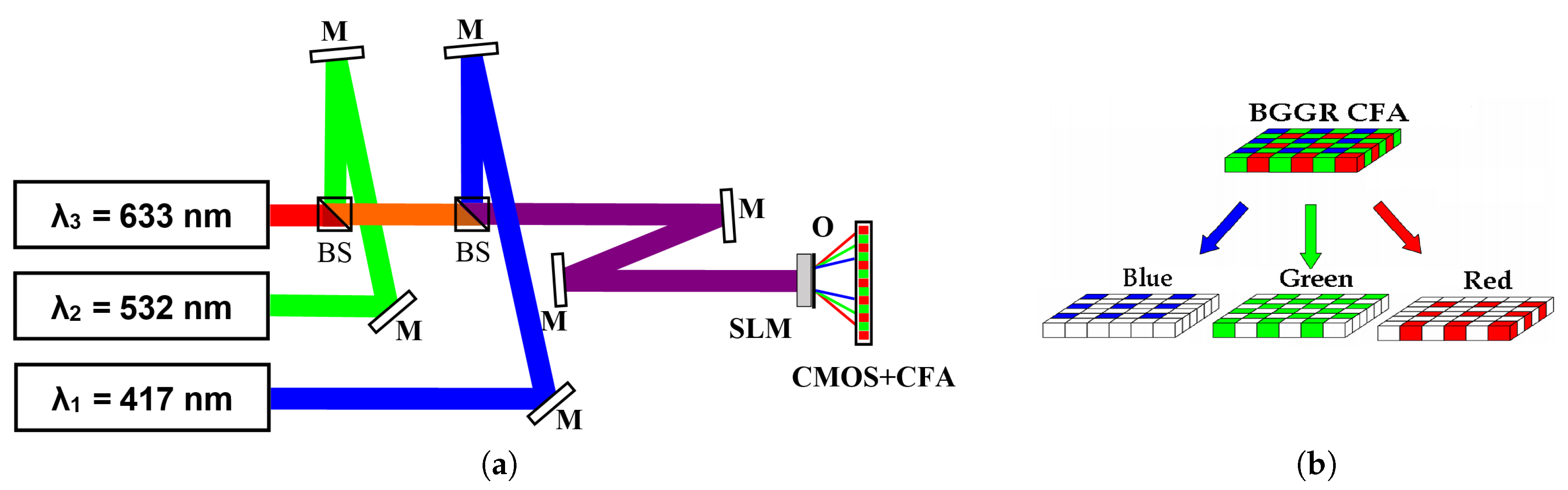
In numerical experiments, we model the lensless optical system (Figure 1a), where a thin transparent phase object is illuminated by monochromatic three color (RGB) coherent light beams from lasers. The wavelengths are , 532, nm with the corresponding refractive indexes [1.528, 1.519, 1.515] as taken for BK7 optical glass. The reference wavelength is nm, then the relative wavelengths are . The pixel sizes of CMOS camera and SLM are 1.4 and 5.6 m, respectively. The distance d between the object and CMOS camera is equal to 5 mm. Figure 1b illustrates arrangement for each color channel of the CMOS camera [64].
A free propagation of the wavefronts from the object to the sensor is given by the Rayleigh-Sommerfeld model with the transfer function defined through the angular spectrum (AS) [65].
For the proper numerical AS propagation without aliasing effects, we introduce a zero-padding in the object plane of the size obtained from the inequality:
which binds the propagation distance d, the number of pixels N in one dimension of the zero-padded object and the pixel size of the sensor [66]. For the distance mm and the object pixels, the zero-padded object has as a support pixels.
The intensities of the light beams registered on the sensor are calculated as , , .
Here denotes the AS propagation operator and are the modulation phase masks inserted before the object and pixelated as the object, stands for pixel-wise multiplication of the object and phase masks. These phase masks enable strong diffraction of the wavefield introduced in order to achieve the phase diversity sufficient for reconstruction of the complex-valued object from intensity measurements. As it was described in [34], we use the Gaussian random phase masks. These phase masks are implemented on SLM. It follows that the pixels of these masks and SLM have the same size.
Thus, in our experiments the propagation operator in Equation (4) is implemented as a combination of the angular spectrum propagation and the modulation phase mask .
To produce multiwavelength color images we need the three color components at each pixel location. It can be achieved by three sensors, each of which registers a light of the specific color. This optical setup for absolute phase retrieval from multiwavelength observations has been studied in our paper [52].
To reduce the complexity and the cost, most digital cameras use a single sensor covered by CFAs. In our simulation we assume that the popular RGB Bayer CFA pattern is used. The corresponding sampled color values are termed mosaic images, Figure 1. To render a full-color pattern at the sensor plane from these CFA samples, an image reconstruction process is applied as defined by Equation (15).
4.2. Reconstruction Results
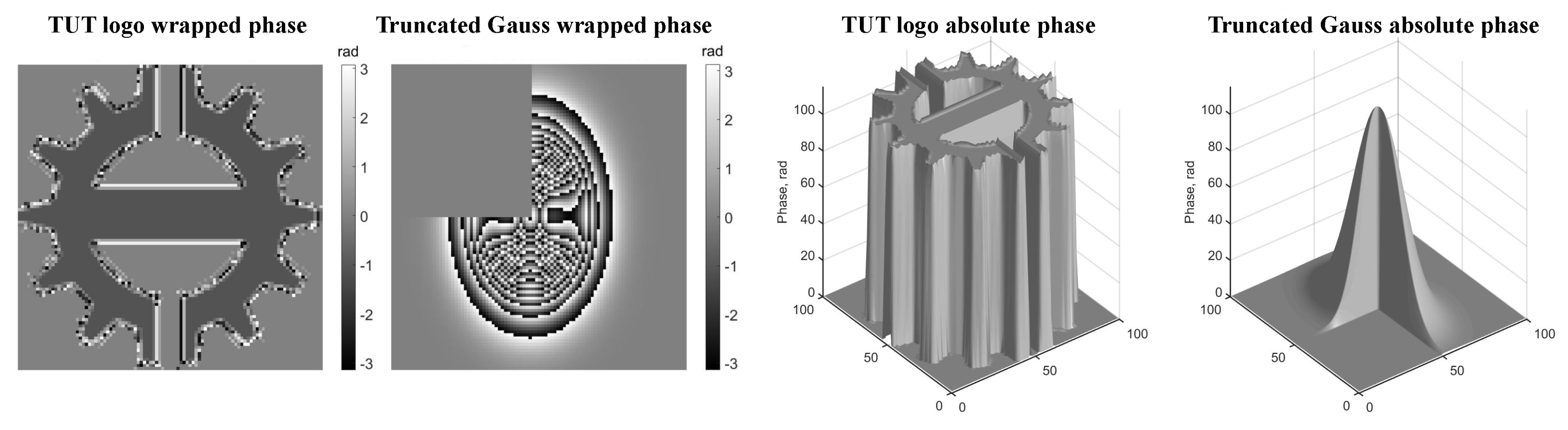
The illustrating reconstructions are presented for two phase test-objects with the invariant amplitudes equal to 1 and the phases: “truncated Gaussian” and “logo” of Tampere University of Technology (TUT), pixels both. The wrapped and absolute phases of these test-objects are shown in Figure 2. The TUT logo and truncated Gaussian phases are very different, the first one is discontinuous binary and the second one is piecewise-smooth continuous. The both test-objects are taken with a high peak-value of the absolute phase equal to rad, that corresponds to about 35 reference wavelength in variations of the profile .
We demonstrate the performance of the WM-APR algorithm for this quite difficult test-objects provided very noisy Poissonian observations. The noisiness of observations is illustrated by values of (Equation (11)) and (Equation (12)).
The accuracy of the object reconstruction is characterized by Relative Root-Mean-Square Error ( calculated as divided by the root of the mean square power of the true signal:
In this criterion the phase estimate is corrected by the mean value of the error between the estimate and true absolute phase. It is the standard approach to evaluation of the accuracy for the phase retrieval, where the phase is estimated within an invariant error.
Note, that values of are identical for accuracy of the phase and the profile . It happens because these variables are different only by the invariant factors, which are the same in nominator and denominator of .
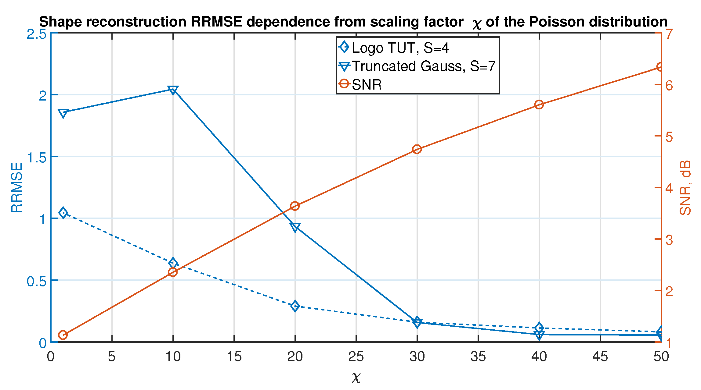
Figure 3 shows the performance of the developed WM-APR algorithm for different noise levels by a dependence of from the noisiness parameter . The curves for truncated Gaussian and logo TUT are given for different numbers of experiments and , respectively. They demonstrate a similar behavior: go down for growing and take values about 0.1 at , what corresponds to the very noisy observed data with a low value of dB and small mean photon number .
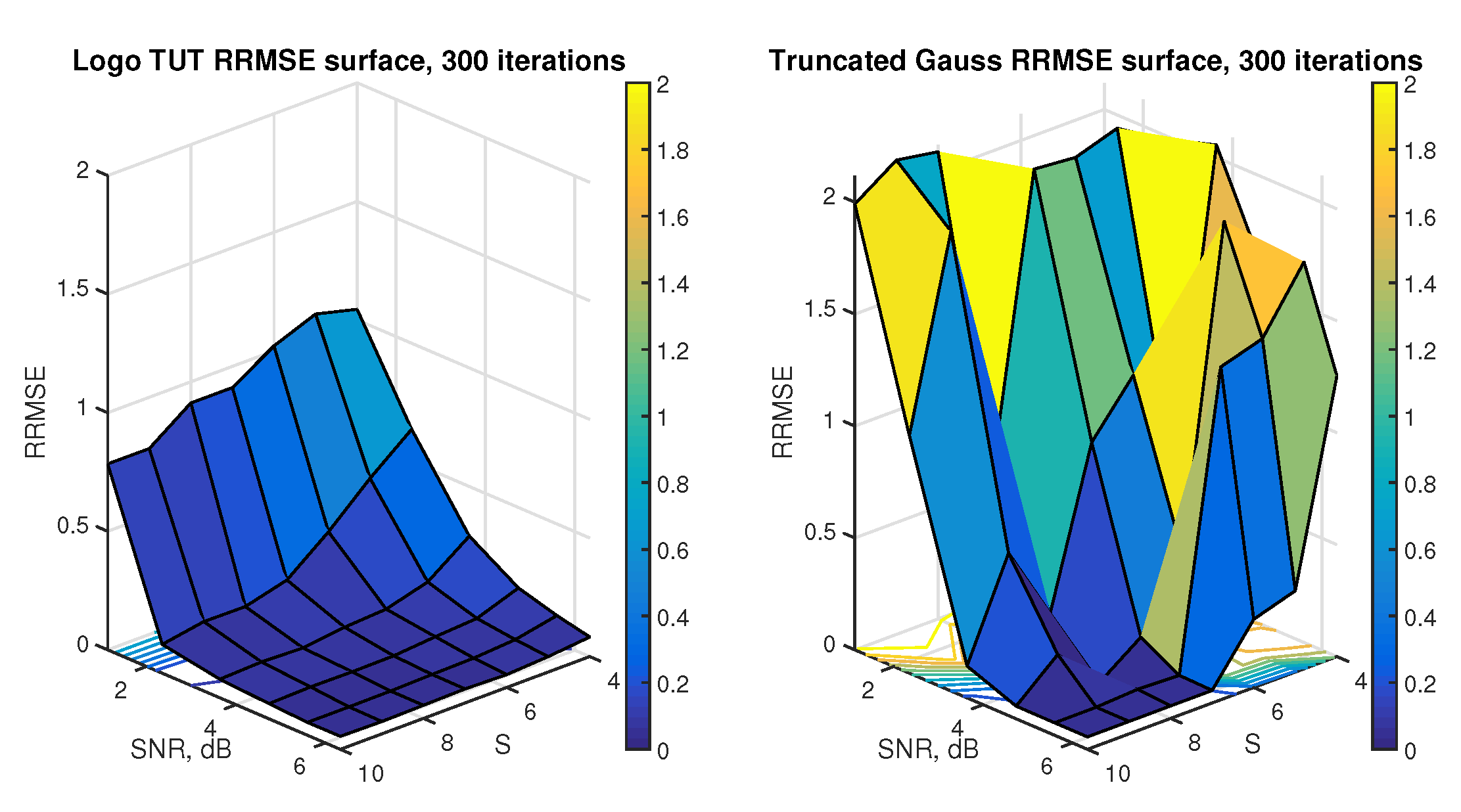
for the logo TUT and Gaussian phases are shown in Figure 4 as functions of the experiment number S and after 300 iterations. Nearly horizontal areas (dark blue in color images) correspond to high-accuracy reconstructions with small values of , for other areas values are much higher and the accuracy is not so good.
As it can be seen from these maps, reconstruction results for logo TUT demonstrate good small values in wide ranges of and S, while truncated Gaussian has such small values only for and . It can be explained by a complex structure of the wrapped phase of the truncated Gaussian phase. It follows from Figure 4, that some improvement in the accuracy can be achieved at the price of the larger number of experiments S.
In what follows, we provide the images of the reconstructed absolute phases obtained for the iteration number , and for logo TUT and truncated Gaussian objects, respectively. The high iteration number is governed by complexity of reconstruction from the CFA mosaic observations, where each pixel of the sensor captures only one red, green or blue color-channel information.
It means that the color information is subsampled with the subsampling ratio 50% for green and 25% for red and blue channels. The missed color-information is restored for each pixel of the sensor (demosaiced) in the iterations of the algorithm as defined by Equations (15)–(17).
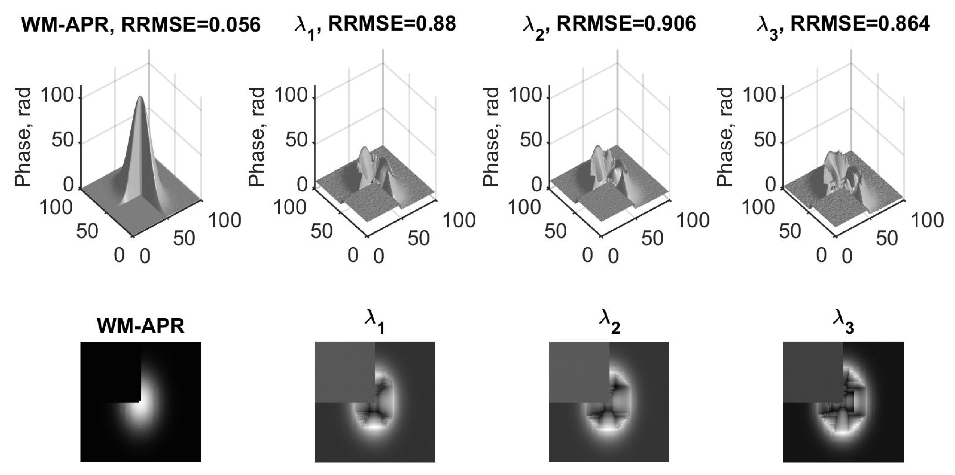
Figure 5 and Figure 6 illustrate the absolute phase reconstruction (3D/2D images) obtained in two different ways: by the proposed WM-APR algorithm and by the SPAR algorithm reconstructing the wrapped phases for the separate wavelength channels following by the phase unwrapping using the PUMA algorithm [42]. The conditions of these experiments are: dB, for both test-objects.
The multiwavelength WM-APR algorithm demonstrates a clear strong advantage in reconstruction of the absolute phases while the processing based on separate wavelength channels completely failed. The accuracy of the WM-APR reconstructions is very high despite of the very noisy observations.
The wrapped phase for the true truncated Gaussian phase should have a form of circular fringes for the parts of the image corresponding to the Gaussian peak. Instead of it in Figure 2, we can see quite irregular structures which look like destroyed by random errors or moiré patterns. This disturbance of the ideal circular fringes is an aliasing effect due to discretization (sampling) of the continuous Gaussian phase with a low sampling rate, which does not satisfy the Nyquist–Shannon conditions. It happens because the peak value of the truncated Gaussian phase is very high and the number of samples (100 × 100) is comparatively small.
This aliasing disturbance of the Gaussian phase is so strong that even advanced 2D unwrapping algorithms, in particular, the PUMA algorithm, failed to reconstruct the absolute truncated Gaussian phase from the precisely noiseless sampled data shown in Figure 2. The impressive high-accuracy performance of the proposed WM-APR algorithm in this extra difficult situation is amazing as demonstrating a strong robustness of this algorithm with respect to errors caused by aliasing effects.
The reconstruction of the absolute phase for the binary logo TUT is also very difficult, in particular, due to huge differences of the phase values for adjacent pixels in the areas of the discontinuity of the phase. The sampling (pixelation) of this absolute phase also leads to the strong aliasing which can be noticed in 2D image in Figure 2. Again the unwrapping of the true noiseless wrapped phase by the 2D unwrapping algorithms is not possible, and then, the fail of the single wavelength based algorithms in Figure 6 is not surprising.
Again, the amazing success of the WM-APR algorithm demonstrates that it is robust with respect to the sampling effects and is able to achieve the high-accuracy reconstruction in very difficult noisy scenarios.
In conclusion, we wish to note that the pair-wise beat-frequency synthetic wavelengths, one of the conventional methods for phase retrieval from multiwavelength observations (e.g., [43,46]), do not work in the considered scenario as the differences between the RGB wavelengths are not small.
For simulations we use MATLAB R2016b on a computer with 32 Gb of RAM and CPU with 3.40 GHz Intel® Core™ i7-3770 processor, GFLOPS. The computation complexity of the algorithm is characterized by the time required for processing. For 1 iteration, , and images, zero-padded to , this time equals to 12 s.
5. Conclusions
The multiwavelength absolute phase retrieval from noisy intensity observations is considered. The system is lensless with multiwavelength coherent input light beams and random phase masks applied for wavefront modulation. The light beams are formed by light sources radiating all wavelengths simultaneously and CMOS sensor equipped with a color filter array (CFA) is used for spectral measurements. The developed algorithm is based on maximum likelihood optimization in this way targeted on optimal phase retrieval from noisy observations. The algorithm for the Poissonian and Gaussian noise distribution is presented. The sparse modeling enables a regularization of the inverse imaging problem and efficient suppression of random observation errors by BM3D filtering of phase and amplitude. The effectiveness of the developed WM-APR algorithm is verified by simulation experiments demonstrated in this work only for the Poissonian noise. The high-accuracy performance of the algorithm is achieved for a high-dynamic range of absolute phase variations while the algorithms operating with the single wavelength observations separately failed. Physical experiments are our priorities for a further work. We consider nonidealities of SLM as a phase modulator and the AS propagation operator as the main challenges for the accuracy of profile and absolute phase reconstruction.
Author Contributions
V.K. developed the algorithm; V.K. and I.S. conceived and designed the experiments; I.S. performed the experiments; V.K., I.S., N.V.P., and K.E. analyzed the data and wrote the paper.
Acknowledgments
This work is supported by Academy of Finland, project no. 287150, 2015–2019, Russian Ministry of Education and Science (project within the state mission for institutions of higher education, agreement 3.1893.2017/4.6) and Horizon 2020 TWINN-2015, grant 687328—HOLO.
Conflicts of Interest
The authors declare no conflict of interest. The founding sponsors had no role in the design of the study; in the collection, analyses, or interpretation of data; in the writing of the manuscript, and in the decision to publish the results.
Abbreviations
The following abbreviations are used in this manuscript:
| CFA | Color Filter Array |
| CMOS | Complementary Metal Oxide Semiconductor |
| SPAR | Sparse Phase and Amplitude Reconstruction |
| Signal-to-Noise Ratio | |
| APR | Absolute Phase Reconstruction |
| BM3D | Block-Matching 3 Dimensions |
| SLM | Spatial Light Modulator |
| AS | Angular Spectrum |
| TUT | Tampere University of Technology |
| Relative Root Mean Square Error | |
| WM-APR | Wavelength Multiplex Absolute Phase Retrieval |
| GFLOPS | FLoating-point Operations Per Second |
| HOSVD | High-Order Singular Value Decompositions |
Appendix A. Absolute Phase Reconstruction (APR) Algorithm
The minimization of (Equation (21)) on and is an absolute phase estimation (unwrapping) problem where the joint use of the -channels is required.
The algorithm is composed from three successive stages A, B, C. We name this algorithm Absolute phase reconstruction (APR) algorithm.
- Phase synchronization. Let be a reference channel. Define the estimates for in (Equation 21) as followswhere are shifts between the phases of the reference and other channels:and is a hypothetical valued of unknown . One of the goals of this calculations is to reduce a number of unknown phase shifts to a single parameter , i.e., the phase-shift in the reference channel. Note that in the above formulas are known (measured) in the algorithm iterations. Thus, indeed, all are expressed through . The wrapping operator in Equations (A1)–(A2) is used for proper calculation of the wrapped phase and the median averaging in order to get the robust estimate of the invariant .Inserting in Equation (21) we obtain this criterion in the formwhere is given.The meaning of , can be revealed if we assume that all phase-shift estimates are accurate than we can see thatIt follows, thatIf we know that than the perfect phase equalization is produced and .In general case, when , the in-phase situation is not achieved.Going back to the criterion (Equation (A3)) we note that with this compensation it takes the formand using (Equation (A4)) it can be rewritten asThus, the accurate compensation of the phase shifts in the wrapped phases is achieved while the absolute phase can be estimated within an unknown but invariant phase shift . This is not essential error as in the phase retrieval setup, can be estimated only within an invariant shift.
- Minimization of Equation (A8) on gives the estimate of the absolute phase provided given .It has no an analytical solution and is obtained by numerical calculations.The calculations in Equation (A8) are produced pixel-wise for each pixel x independently.Note that as well as the solution both depend on the unknown invariant .
- Finalization of estimation. When is found the optimal values for are calculated asIn our algorithm implementation, the solutions for Equations (A6) and (A9) are obtained by the grid optimization.It has been noted in our experiments that an essential improvement in the accuracy of the absolute phase reconstruction is achieved due to optimization on .
References
- Picart, P.; Li, J. Digital Holography; John Wiley & Sons: Hoboken, NJ, USA, 2013. [Google Scholar]
- Schnars, U.; Falldorf, C.; Watson, J.; Jüptner, W. Digital Holography and Wavefront Sensing; Springer: Berlin/Heidelberg, Germany, 2015. [Google Scholar]
- Belashov, A.; Petrov, N.; Semenova, I. Digital off-axis holographic interferometry with simulated wavefront. Opt. Express 2014, 22, 28363–28376. [Google Scholar] [CrossRef] [PubMed]
- Belashov, A.V.; Petrov, N.V.; Semenova, I.V. Accuracy of image-plane holographic tomography with filtered backprojection: random and systematic errors. Appl. Opt. 2016, 55, 81–88. [Google Scholar] [CrossRef] [PubMed]
- Kostencka, J.; Kozacki, T. Space-domain, filtered backpropagation algorithm for tomographic configuration with scanning of illumination. Int. Soc. Opt. Photonics 2016, 9890, 98900F. [Google Scholar]
- Wu, C.H.; Lai, X.J.; Cheng, C.J.; Yu, Y.C.; Chang, C.Y. Applications of digital holographic microscopy in therapeutic evaluation of Chinese herbal medicines. Appl. Opt. 2014, 53, G192–G197. [Google Scholar] [CrossRef] [PubMed]
- Belashov, A.V.; Zhikhoreva, A.A.; Belyaeva, T.N.; Kornilova, E.S.; Petrov, N.V.; Salova, A.V.; Semenova, I.V.; Vasyutinskii, O.S. Digital holographic microscopy in label-free analysis of cultured cells’ response to photodynamic treatment. Opt. Lett. 2016, 41, 5035. [Google Scholar] [CrossRef] [PubMed]
- Cheremkhin, P.A.; Evtikhiev, N.N.; Krasnov, V.V.; Kulakov, M.N.; Kurbatova, E.A.; Molodtsov, D.Y.; Rodin, V.G. Demonstration of digital hologram recording and 3D-scenes reconstruction in real-time. Int. Soc. Opt. Photonics 2016, 9889, 98891M. [Google Scholar]
- Coppola, G.; Ferraro, P.; Iodice, M.; Nicola, S.D.; Finizio, A.; Grilli, S. A digital holographic microscope for complete characterization of microelectromechanical systems. Meas. Sci. Technol. 2004, 15, 529–539. [Google Scholar] [CrossRef]
- Gerchberg, R.W.; Saxton, W.O. A Practical Algorithm for the Determination of Phase from Image and Diffraction Plane Pictures. Optik 1969, 35, 237–246. [Google Scholar]
- Fienup, J.R. Phase retrieval algorithms: a comparison. Appl. Opt. 1982, 21, 2758. [Google Scholar] [CrossRef] [PubMed]
- Almoro, P.F.; Pedrini, G.; Gundu, P.N.; Osten, W.; Hanson, S.G. Enhanced wavefront reconstruction by random phase modulation with a phase diffuser. Opt. Lasers Eng. 2011, 49, 252–257. [Google Scholar] [CrossRef]
- Candès, E.J.; Li, X.; Soltanollotabi, M. Phase Retrieval from Coded Difraction Patterns. arXiv 2013, arXiv:1310.32402013, 1–24. [Google Scholar]
- Almoro, P.F.; Pham, Q.D.; Serrano-Garcia, D.I.; Hasegawa, S.; Hayasaki, Y.; Takeda, M.; Yatagai, T. Enhanced intensity variation for multiple-plane phase retrieval using a spatial light modulator as a convenient tunable diffuser. Opt. Lett. 2016, 41, 2161. [Google Scholar] [CrossRef] [PubMed]
- Camacho, L.; Micó, V.; Zalevsky, Z.; García, J. Quantitative phase microscopy using defocusing by means of a spatial light modulator. Opt. Express 2010, 18, 6755–6766. [Google Scholar] [CrossRef] [PubMed]
- Kress, B.C.; Meyrueis, P. Applied Digital Optics—From Micro Optics to Nanophotonics; John Wiley & Sons: Hoboken, NJ, USA, 2009; p. 617. [Google Scholar]
- Guo, C.; Liu, S.; Sheridan, J.T. Iterative phase retrieval algorithms I: Optimization. Appl. Opt. 2015, 54, 4698. [Google Scholar] [CrossRef] [PubMed]
- Fienup, J.R. Phase-retrieval algorithms for a complicated optical system. Appl. Opt. 1993, 32, 1737. [Google Scholar] [CrossRef] [PubMed]
- Bauschke, H.H.; Combettes, P.L.; Luke, D.R. Phase retrieval, error reduction algorithm, and Fienup variants: a view from convex optimization. J. Opt. Soc. Am. A 2002, 19, 1334. [Google Scholar] [CrossRef]
- Pauwels, E.; Beck, A.; Eldar, Y.C.; Sabach, S. On Fienup Methods for Regularized Phase Retrieval. arXiv, 2017; arXiv:1702.08339. [Google Scholar]
- Shechtman, Y.; Eldar, Y.C.; Cohen, O.; Chapman, H.N.; Miao, J.; Segev, M. Phase Retrieval with Application to Optical Imaging: A contemporary overview. IEEE Signal Process. Mag. 2015, 32, 87–109. [Google Scholar] [CrossRef]
- Yurtsever, A.; Udell, M.; Tropp, J.A.; Cevher, V. Sketchy Decisions: Convex Low-Rank Matrix Optimization with Optimal Storage. arXiv, 2017; arXiv:1702.06838. [Google Scholar]
- Candès, E.J.; Li, X.; Soltanolkotabi, M. Phase Retrieval via Wirtinger Flow: Theory and Algorithms. IEEE Trans. Inf. Theory 2015, 61, 1985–2007. [Google Scholar] [CrossRef]
- Chen, Y.; Candès, E.J. Solving Random Quadratic Systems of Equations Is Nearly as Easy as Solving Linear Systems. Commun. Pure Appl. Math. 2017, 70, 822–883. [Google Scholar] [CrossRef]
- Weller, D.S.; Pnueli, A.; Divon, G.; Radzyner, O.; Eldar, Y.C.; Fessler, J.A. Undersampled Phase Retrieval With Outliers. IEEE Trans. Comput. Imaging 2015, 1, 247–258. [Google Scholar] [CrossRef] [PubMed]
- Soulez, F.; Thiébaut, É.; Schutz, A.; Ferrari, A.; Courbin, F.; Unser, M. Proximity operators for phase retrieval. Appl. Opt. 2016, 55, 7412. [Google Scholar] [CrossRef] [PubMed]
- Shechtman, Y.; Beck, A.; Eldar, Y.C. GESPAR: Efficient phase retrieval of sparse signals. IEEE Trans. Signal Process. 2014, 62, 928–938. [Google Scholar] [CrossRef]
- Tillmann, A.M.; Eldar, Y.C.; Mairal, J. DOLPHIn—Dictionary Learning for Phase Retrieval. IEEE Trans. Signal Process. 2016, 64, 6485–6500. [Google Scholar] [CrossRef] [Green Version]
- Katkovnik, V.; Astola, J. High-accuracy wave field reconstruction: Decoupled inverse imaging with sparse modeling of phase and amplitude. J. Opt. Soc. Am. A 2012, 29, 44–54. [Google Scholar] [CrossRef] [PubMed]
- Katkovnik, V.; Astola, J. Compressive sensing computational ghost imaging. J. Opt. Soc. Am. A 2012, 29, 1556. [Google Scholar] [CrossRef] [PubMed]
- Katkovnik, V.; Astola, J. Sparse ptychographical coherent diffractive imaging from noisy measurements. J. Opt. Soc. Am. A Opt. Image Sci. Vis. 2013, 30, 367–379. [Google Scholar] [CrossRef] [PubMed]
- Katkovnik, V. Phase retrieval from noisy data based on sparse approximation of object phase and amplitude. arXiv, 2017; arXiv:1709.01071. [Google Scholar]
- Katkovnik, V.; Egiazarian, K. Sparse superresolution phase retrieval from phase-coded noisy intensity patterns. Opt. Eng. 2017, 56, 094103. [Google Scholar] [CrossRef]
- Katkovnik, V.; Shevkunov, I.; Petrov, N.; Egiazarian, K. Computational super-resolution phase retrieval from multiple phase-coded diffraction patterns: Simulation study and experiments. Optica 2017, 4, 786–794. [Google Scholar] [CrossRef]
- Towers, C.E.; Towers, D.P.; Jones, J.D.C. Absolute fringe order calculation using optimised multi-frequency selection in full-field profilometry. Opt. Lasers Eng. 2005, 43, 52–64. [Google Scholar] [CrossRef]
- Pedrini, G.; Osten, W.; Zhang, Y. Wave-front reconstruction from a sequence of interferograms recorded at different planes. Opt. Lett. 2005, 30, 833–835. [Google Scholar] [CrossRef] [PubMed]
- Falldorf, C.; Huferath-von Luepke, S.; von Kopylow, C.; Bergmann, R.B. Reduction of speckle noise in multiwavelength contouring. Appl. Opt. 2012, 51, 8211. [Google Scholar] [CrossRef] [PubMed]
- Cheremkhin, P.; Shevkunov, I.; Petrov, N. Multiple-wavelength Color Digital Holography for Monochromatic Image Reconstruction. Phys. Procedia 2015, 73, 301–307. [Google Scholar] [CrossRef]
- Tahara, T.; Otani, R.; Arai, Y.; Takaki, Y. Multiwavelength Digital Holography and Phase-Shifting Interferometry Selectively Extracting Wavelength Information: Phase-Division Multiplexing (PDM) of Wavelengths. Hologr. Mater. Opt. Syst. 2017, 25, 11157–11172. [Google Scholar]
- Claus, D.; Pedrini, G.; Buchta, D.; Osten, W. Spectrally resolved digital holography using a white light LED. Proc. SPIE–Int. Soc. Opt. Eng. 2017, 10335, 103351H. [Google Scholar]
- Bioucas-Dias, J.; Katkovnik, V.; Astola, J.; Egiazarian, K. Multi-frequency Phase Unwrapping from Noisy Data: Adaptive Local Maximum Likelihood Approach RID C-5479-2009. Image Anal. Proc. 2009, 5575, 310–320. [Google Scholar]
- Bioucas-Dias, J.; Valadão, G. Multifrequency absolute phase estimation via graph cuts. In Proceedings of the 2009 17th European Signal Processing Conference, Glasgow, UK, 24–28 August 2009; pp. 1389–1393. [Google Scholar]
- Bao, P.; Zhang, F.; Pedrini, G.; Osten, W. Phase retrieval using multiple illumination wavelengths. Opt. Lett. 2008, 33, 309–311. [Google Scholar] [CrossRef] [PubMed]
- Petrov, N.V.; Bespalov, V.G.; Gorodetsky, A.A. Phase retrieval method for multiple wavelength speckle patterns. Proc. SPIE 2010, 7387, 73871T. [Google Scholar]
- Petrov, N.V.; Volkov, M.V.; Gorodetsky, A.A.; Bespalov, V.G. Image reconstruction using measurements in volume speckle fields formed by different wavelengths. Proc. SPIE 2011, 7907, 790718. [Google Scholar]
- Bao, P.; Situ, G.; Pedrini, G.; Osten, W. Lensless phase microscopy using phase retrieval with multiple illumination wavelengths. Appl. Opt. 2012, 51, 5486–5494. [Google Scholar] [CrossRef] [PubMed]
- Phillips, Z.F.; Chen, M.; Waller, L. Single-shot quantitative phase microscopy with color-multiplexed differential phase contrast (cDPC). PLoS ONE 2017, 12, e0171228. [Google Scholar] [CrossRef] [PubMed]
- Sanz, M.; Picazo-Bueno, J.A.; García, J.; Micó, V. Improved quantitative phase imaging in lensless microscopy by single-shot multi-wavelength illumination using a fast convergence algorithm. Opt. Express 2015, 23, 21352–21365. [Google Scholar] [CrossRef] [PubMed]
- Falaggis, K.; Towers, D.P.; Towers, C.E. Algebraic solution for phase unwrapping problems in multiwavelength interferometry. Appl. Opt. 2014, 53, 3737. [Google Scholar] [CrossRef] [PubMed]
- Wang, W.; Li, X.; Wang, W.; Xia, X.G. Maximum likelihood estimation based Robust Chinese remainder theorem for real numbers and its fast algorithm. IEEE Trans. Signal Process. 2015, 63, 3317–3331. [Google Scholar] [CrossRef]
- Xiao, L.; Xia, X.G.; Huo, H. Towards Robustness in Residue Number Systems. IEEE Trans. Signal Process. 2016, 65, 1–32. [Google Scholar] [CrossRef]
- Katkovnik, V.; Shevkunov, I.; Petrov, N.V.; Egiazarian, K. Multiwavelength surface contouring from phase-coded diffraction patterns. Presented at SPIE Photonics Europe, Palais de la Musique et des Congrès, Strasbourg, France, 22–26 April 2018. Paper 10677-46. [Google Scholar]
- Kulya, M.S.; Balbekin, N.S.; Gredyuhina, I.V.; Uspenskaya, M.V.; Nechiporenko, A.P.; Petrov, N.V. Computational terahertz imaging with dispersive objects. J. Mod. Opt. 2017, 64, 1283–1288. [Google Scholar] [CrossRef]
- Dabov, K.; Foi, A.; Katkovnik, V. Image denoising by sparse 3D transformation-domain collaborative filtering. IEEE Trans. Image Process. 2007, 16, 2080–2095. [Google Scholar] [CrossRef] [PubMed]
- Lesnichii, V.V.; Petrov, N.V.; Cheremkhin, P.A. A technique of measuring spectral characteristics of detector arrays in amateur and professional photocameras and their application for problems of digital holography. Opt. Spectrosc. 2013, 115, 557–566. [Google Scholar] [CrossRef]
- Raginsky, M.; Willett, R.; Harmany, Z.; Marcia, R. Compressed sensing performance bounds under Poisson noise. Signal Process. IEEE Trans. 2010, 58, 3990–4002. [Google Scholar] [CrossRef]
- Harmany, Z.T.; Marcia, R.F.; Willett, R.M. Sparsity-regularized photon-limited imaging. In Proceedings of the 2010 IEEE International Symposium on Biomedical Imaging: From Nano to Macro, Rotterdam, The Netherlands, 14–17 April 2010; pp. 772–775. [Google Scholar]
- Mallat, S.G. A Theory for Multiresolution Signal Decomposition: The Wavelet Representation. IEEE Trans. Pattern Anal. Mach. Intell. 1989, 11, 674–693. [Google Scholar] [CrossRef]
- Rajwade, A.; Member, S.; Rangarajan, A. Image Denoising Using the Higher Order Singular Value Decomposition. IEEE Trans. Pattern Anal. Mach. Intell. 2013, 35, 849–862. [Google Scholar] [CrossRef] [PubMed]
- Metzler, C.A.; Maleki, A.; Baraniuk, R.G. BM3D-PRGAMP: Compressive phase retrieval based on BM3D denoising. In Proceedings of the 2016 IEEE International Conference on Image Processing (ICIP), Phoenix, AZ, USA, 25–28 September 2016; pp. 2504–2508. [Google Scholar]
- Danielyan, A.; Katkovnik, V.; Egiazarian, K. BM3D Frames and Variational Image Deblurring. IEEE Trans. Image Process. 2012, 21, 1715–1728. [Google Scholar] [CrossRef] [PubMed]
- Katkovnik, V.; Shevkunov, I.A.; Petrov, N.V.; Egiazarian, K. Wavefront reconstruction in digital off-axis holography via sparse coding of amplitude and absolute phase. Opt. Lett. 2015, 40, 2417. [Google Scholar] [CrossRef] [PubMed]
- Katkovnik, V.; Ponomarenko, M.; Egiazarian, K. Sparse approximations in complex domain based on BM3D modeling. Signal Process. 2017, 141, 96–108. [Google Scholar] [CrossRef]
- Cheremkhin, P.A.; Lesnichii, V.V.; Petrov, N.V. Use of spectral characteristics of DSLR cameras with Bayer filter sensors. J. Phys. Conf. Ser. 2014, 536, 012021. [Google Scholar] [CrossRef]
- Goodman, J.W. Introduction to Fourier opt.; Roberts & Co.: Greenwood Village, CO, USA, 2005; p. 491. [Google Scholar]
- Petrov, N.V.; Bespalov, V.G.; Volkov, M.V. Phase retrieval of THz radiation using set of 2D spatial intensity measurements with different wavelengths. Proc. SPIE 2012, 8281, 82810J. [Google Scholar]
Figure 1.
(a) Optical setup. nm, nm, nm are wavelengths of the blue, green, and red light sources, M are mirrors, BS are beam-splitters, SLM stands for Spatial Light Modulator, O is the object, CMOS+CFA is a registration camera with CFA; (b) Color filter array. BGGR CFA is a blue-green-green-red disposed CFA; Blue, Green and Red are separate color channels.

Figure 2.
Wrapped and absolute phases of the investigated test-objects: truncated Gaussian and TUT logo, the reference wavelength .
Figure 2.
Wrapped and absolute phases of the investigated test-objects: truncated Gaussian and TUT logo, the reference wavelength .

Figure 3.
and as functions of the parameter of the Poissonian distribution: solid triangles and dashed diamonds curves (blue in color images) show for the truncated Gaussian and logo TUT objects, respectively (left y-axis); solid circle curve (orange) shows of the observations (right y-axis).
Figure 3.
and as functions of the parameter of the Poissonian distribution: solid triangles and dashed diamonds curves (blue in color images) show for the truncated Gaussian and logo TUT objects, respectively (left y-axis); solid circle curve (orange) shows of the observations (right y-axis).

Figure 4.
as functions of and the number of experiments S, 300 iterations, left and right 3D images are for Logo TUT and truncated Gaussian, respectively.
Figure 4.
as functions of and the number of experiments S, 300 iterations, left and right 3D images are for Logo TUT and truncated Gaussian, respectively.

Figure 5.
Truncated Gaussian absolute phase reconstructions: (, ), top row - 3D absolute phase surfaces, bottom row - the corresponding 2D absolute phase images. From left to right: WM-APR algorithm, and phase reconstructions obtained separately for , , wavelengths, respectively, followed by the 2D phase unwrapping.

Figure 6.
Logo TUT phase reconstructions: (, ), (top row)—3D absolute phase surfaces, (bottom row)—the corresponding 2D absolute phases images. From left to right: WM-APR algorithm, and phase reconstructions obtained separately for , , wavelengths, respectively, followed by the 2D phase unwrapping.
Figure 6.
Logo TUT phase reconstructions: (, ), (top row)—3D absolute phase surfaces, (bottom row)—the corresponding 2D absolute phases images. From left to right: WM-APR algorithm, and phase reconstructions obtained separately for , , wavelengths, respectively, followed by the 2D phase unwrapping.


Table 1.
Wavelength Multiplexing Absolute Phase Retrieval (WM-APR) Algorithm.
| Input:, , | |
| Initialization:, | |
| Main iterations: | |
| 1. | Forward propagation and mixing |
| , | |
| ; | |
| 2. | Noise suppression: |
| ; | |
| 3. | Backward propagation and filtering: |
| , | |
| 4. | Absolute phase retrieval and filtering: |
| {; | |
| 5. | Object wavefront update: |
| Output |
© 2018 by the authors. Licensee MDPI, Basel, Switzerland. This article is an open access article distributed under the terms and conditions of the Creative Commons Attribution (CC BY) license (http://creativecommons.org/licenses/by/4.0/).
Share and Cite
MDPI and ACS Style
Katkovnik, V.; Shevkunov, I.; Petrov, N.V.; Eguiazarian, K. Multiwavelength Absolute Phase Retrieval from Noisy Diffractive Patterns: Wavelength Multiplexing Algorithm. Appl. Sci. 2018, 8, 719. https://doi.org/10.3390/app8050719
AMA Style
Katkovnik V, Shevkunov I, Petrov NV, Eguiazarian K. Multiwavelength Absolute Phase Retrieval from Noisy Diffractive Patterns: Wavelength Multiplexing Algorithm. Applied Sciences. 2018; 8(5):719. https://doi.org/10.3390/app8050719
Chicago/Turabian StyleKatkovnik, Vladimir, Igor Shevkunov, Nikolay V. Petrov, and Karen Eguiazarian. 2018. "Multiwavelength Absolute Phase Retrieval from Noisy Diffractive Patterns: Wavelength Multiplexing Algorithm" Applied Sciences 8, no. 5: 719. https://doi.org/10.3390/app8050719
Note that from the first issue of 2016, this journal uses article numbers instead of page numbers. See further details here.