
The Aerodynamic Analysis of a Rotating Wind Turbine by Viscous-Coupled 3D Panel Method


1
Department of Engineering Science and Ocean Engineering, National Taiwan University, Taipei 106, Taiwan
2
Research Department, CR Classification Society, 8th Fl., No. 103, Sec. 3, Nanking E. Rd., Taipei 104, Taiwan
*
Author to whom correspondence should be addressed.
Appl. Sci. 2017, 7(6), 551; https://doi.org/10.3390/app7060551
Submission received: 11 March 2017
/
Revised: 18 May 2017
/
Accepted: 22 May 2017
/
Published: 26 May 2017
(This article belongs to the Section Energy Science and Technology)
Abstract
:In addition to the many typical failure mechanisms that afflict wind turbines, units in Taiwan are also susceptible to catastrophic failure from typhoon-induced extreme loads. A key component of the strategy to prevent such failures is a fast, accurate aerodynamic analysis tool through which a fuller understanding of aerodynamic loads acting on the units may be derived. To this end, a viscous-coupled 3D panel method is herewith proposed, which introduces a novel approach to simulating the severe flow separation so prevalent around wind turbine rotors. The validity of the current method’s results was assessed by code-to-code comparison with RANS data for a commercial 2 MW wind turbine rotor. Along the outboard and inboard regions of the rotor, pressure distributions predicted by the current method showed excellent agreement with the RANS data, while pressure data along the midspan region were slightly more conservative. The power curve predicted by the current method was also more conservative than that predicted by the RANS solver, but correlated very well with that provided by the turbine manufacturer. Taking into account the high degree of comparability with the more sophisticated RANS solver, the excellent agreement with the official data, and the considerably reduced computational expense, the author believes the proposed method could be a powerful standalone tool for the design and analysis of wind turbine blades, or could be applied to the emerging field of wind farm layout design by providing accurate body force input to actuator line rotors within full Navier-Stokes models of multi-unit wind farms.
Keywords:
CFD; panel method; boundary layer; flow separation; thick wake; actuator line model; wind farm1. Introduction
The Pacific island nation of Taiwan, having abundant wind energy resources, stable wind speed and direction, and shallow water depth, is listed by 4C Offshore Limited as one of the world’s best offshore wind farm locations [1]. Taiwan has duly “pledged to boost [its] offshore wind industry by investing NT$ 88 billion (US$ 2.9 billion) by 2020 and NT$ 670 billion (US$ 21.7 billion) by 2030” [2]. The island, however, being located in the northwestern Pacific tropical cyclone basin, is struck by an average of four typhoons per year, resulting in average annual total losses of NT$ 15 billion [3]. In August, 2015, Typhoon Soudelor alone destroyed eight wind turbines, causing “an estimated NT$ 560 million (US$ 18.2 million) in damages” [4]. The proposed wind farm units, in addition to the many typical failure mechanisms that afflict wind turbines in wind farms, such as exacerbated fatigue loading due to unsteady wind farm wake effects [5], will, therefore, also have to withstand typhoon-induced extreme loads.
To better design for the wide range of loading conditions facing Taiwan’s wind turbines, a fast, versatile CFD tool is desired, one which is able to handle the many challenges associated with the aerodynamic analysis of wind turbines, such as rotor rotation, rotor-tower interaction, wind shear, fluctuations in wind speed and direction, both ambient and self-generated (in-farm), aeroelasticity, and flow separation, which is unavoidable close to the blade root where:
- (1)
- aerodynamic efficiency is sacrificed in favour of greater structural integrity; and
- (2)
- local tip speed ratios decrease with decreasing radial distance, resulting in higher angles of relative wind, and, typically, higher angles of attack.
The CFD analysis of these detached flow problems is especially troublesome, necessitating a solution of the viscous boundary layer, which is achieved, in Reynolds-averaged Navier-Stokes (RANS) solvers, by very fine and therefore computationally expensive mesh resolutions near the wall, or, in potential flow solvers (panel methods), through empirical viscous corrections. RANS solvers, however, “with their long computation times, which are typically in the order of hours [or even days for more complicated flow problems], are usually relegated to the post-design analysis of fluid dynamic problems, [while the] fast computation times of panel methods—in the order of seconds—make them an excellent CFD tool at the preliminary design stage” [6]. A further advantage of panel methods over RANS solvers is that with the latter, a significant amount of time is typically required for preprocessing, such as mesh generation, watertightness testing, the clean-up process for which can involve considerable manual effort, and mesh independence testing. On the other hand, “discretisation [in panel methods] is confined to the object’s surface, allowing for fast, convenient modification of geometric parameters” [6]. Finally, the speed and code-openness of panel methods allow for ease of coupling for such applications as aeroelastic problems, optimisation algorithms, and actuator line models, in which the reaction forces of the rotor on the fluid (equal and opposite to the calculated aerodynamic loads) are imposed on RANS [7,8,9,10] or large eddy simulation (LES) [11,12,13,14,15,16,17] models of the entire computational domain of a wind farm. This actuator line approach allows researchers to investigate the unsteady flow field throughout a wind farm without the associated computational expense of resolving the Navier-Stokes equations around the individual wind turbine units. Such actuator line models usually rely on 2D airfoil characteristics at discrete blade elements for their input body forces, but Dobrev et al. [18] observed “larger deviations [from measured data] at high velocities where the flow field is detached”. The success of the current method in quickly and accurately modelling such detached flows makes it an ideal candidate for these actuator line models.
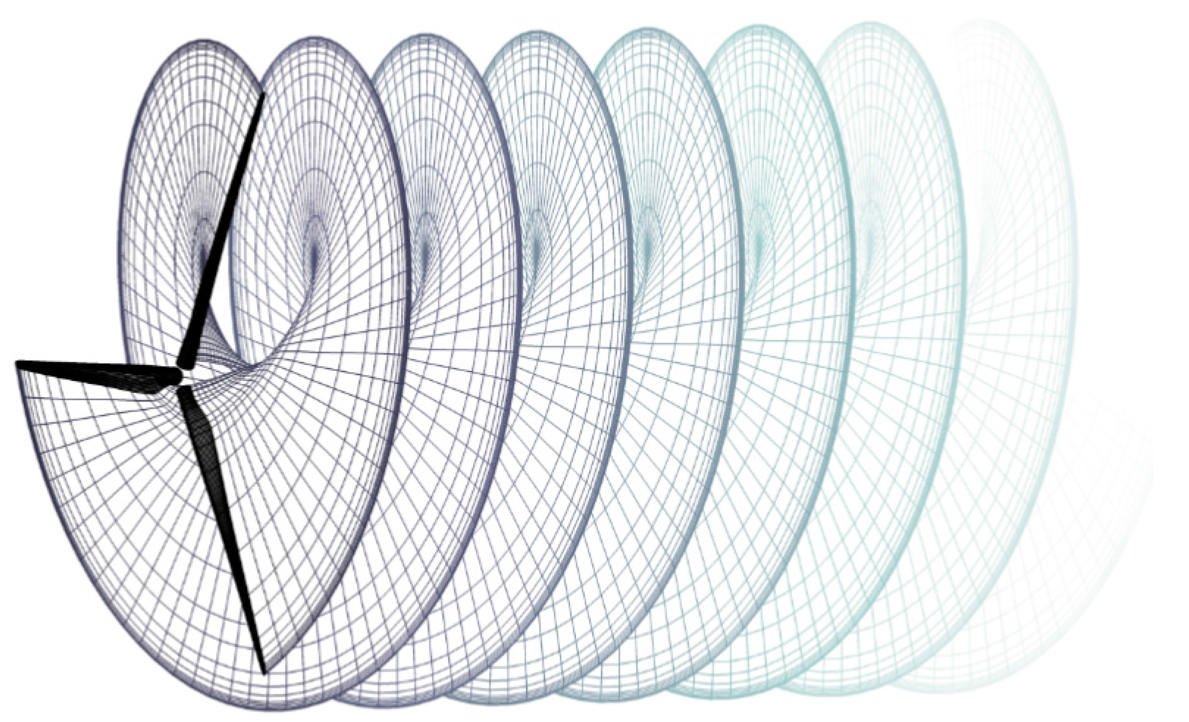
The panel method adopted in the present study is an open-source version of the Hess-Smith panel method [19], which was released by Filkovic [20], and was based on the Fortran code published by Katz and Plotkin [21]. This panel method, which discretises the target body surface into a number of quadrilateral source and doublet distributions, was adapted for the analysis of a full wind turbine rotor by imposing on the free stream wind a rotational component, defined in cylindrical coordinates, and modelling the wake as a sheet of doublet panels extending helically downstream (Figure 1).
Finally, the onset of flow separation, which is unavoidable close to the non-aerodynamic blade root, and may extend along the entire length of the rotor blades at supra-nominal wind speeds, was predicted by a classic integral boundary layer analysis, with the separated wake resolved via the proposed “thick wake” method, which is described in Section 2.3.2.
In the present study, this approach was applied to the aerodynamic analysis of a commercial 2 MW wind turbine rotor under normal operating conditions. Predicted pressure distributions around airfoil sections at several radial locations were compared with RANS data—the model specifications are summarised in Section 3, with detailed discussion to be found in [22]—as well as with Xfoil data for identical 2D airfoils in uniform flow. A predicted output power curve at normal operating wind speeds was compared with the RANS data and with official data provided by the wind turbine manufacturer [23].
2. Numerical Formulation
2.1. Potential Flow
Potential flow theory assumes an inviscid, incompressible (), irrotational () fluid flow , which may, due to irrotationality, be expressed as the gradient of a scalar, i.e., . This scalar, called velocity potential, is substituted into the continuity equation to give us the Laplace equation,
This is the governing equation for potential flow, and two of its solutions are:
which are the potentials for a source σ and a doublet μ. Panel methods are able to simulate the flow fields around arbitrary bodies by exploiting the velocity fields induced by distributions (panels) of such solutions. The perturbation potential at each panel’s centroid is obtained by summing the influences of all body and wake panels:
Differentiating doublet strengths with respect to local coordinates gives the induced velocity field on the body surface, Equation (5), which is then used to obtain the pressure field, Equation (6):
where is the undisturbed relative flow velocity.
2.2. The Boundary Layer
Within the boundary layer, an order of magnitude analysis may be applied to the 2D Navier-Stokes equations to obtain Equations (7) and (8). These two equations, together with the 2D continuity equation, Equation (9), comprise the Prandtl boundary layer equations.
where x is measured parallel to the body surface streamwise, and normal to it.
A few extra parameters which are integral to the description of the boundary layer are the boundary layer displacement thickness , Equation (10), and momentum thickness θ, Equation (11), defined as the distances by which the inviscid surface streamline must be displaced to compensate for, respectively, the reductions in flow rate and total momentum in the boundary layer. The shear stress and skin friction coefficient are defined by Equations (12) and (13),
where is the flow speed outside the boundary layer, predicted by the inviscid analysis, and τw is the shear stress at the body surface.
Substituting Equations (10)–(13) into Equations (7)–(9) gives the von Kármán momentum integral equation:
where is a shape factor. The separation point may be determined by supplementing Equation (14) with additional relations. For the computation of the laminar and turbulent separation points, the present study adopts Thwaites’s [24] and Head’s methods [25], respectively.
By rearranging the von Kármán momentum integral equation, Equation (14), Thwaites showed that θ2 is very well approximated by:
He then introduced a new parameter , which may be calculated via (15), and went on to show that laminar-to-turbulent flow transition occurs at λ < −0.09.
Concerning the turbulent boundary layer, Head considered the entrainment of fluid from the free stream into the turbulent boundary layer, where the entrainment velocity E may be written in terms of the displacement thickness, Equation (16), via a turbulent shape factor, :
The dimensionless entrainment velocity may then be calculated via the following empirical formulae, as fit by Cebeci and Bradshaw [26]:
To solve for cf, Head adopted the Ludwieg-Tillman skin-friction law:
and ordinary differential Equations (15) and (17) are solved for θ and H1 via a 2nd order Runge-Kutta method. Turbulent separation is assumed to occur when H1 falls below 3.3 [27].
2.3. The Separated Wake
2.3.1. The Double Wake Method
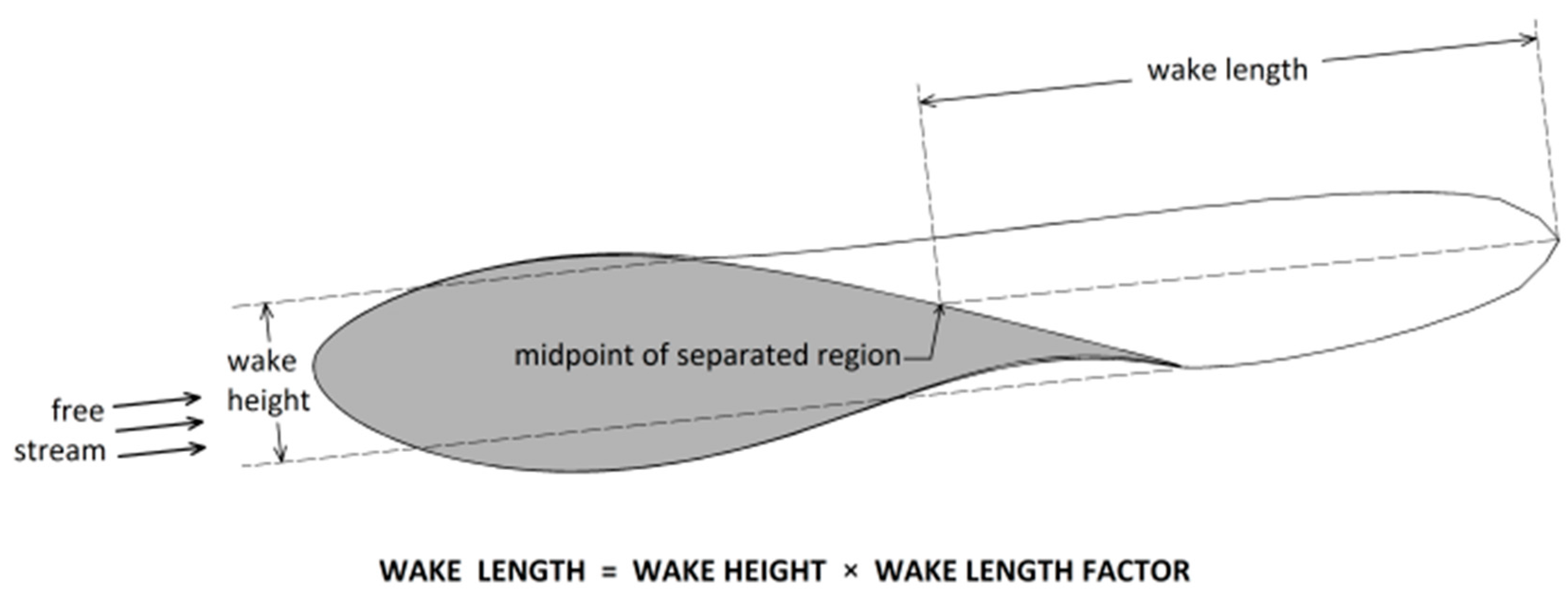
In the late 1970s, Maskew and Dvorak [28] developed a 2D panel method to calculate the flow field around airfoils for angles of attack up to and beyond stall. They treated the separated wake as a region of “constant total pressure bounded by [a pair of] free shear layers” [29]; ergo, this method is typically referred to in the literature as the “double wake” method. Because “the position of the vortex sheets representing the free shear layers is not known a priori” [30], the initial wake shape is “represented by parabolic curves passing from the separation points to a common point [...] on the mean wake line, distance WL downstream from the wake midpoint” [31] (Figure 2). WL, the wake length, is based on a wake length factor, WF ≡ 0.081 × c/t + 1.1 [32], which follows an empirical relationship between the extent of separation (represented as “wake height”) and the thickness-to- chord ratio. The wake panels are then iteratively reoriented until the normal velocities on all wake panels converge to within a tolerance of “1% of the free stream velocity” [29]. However, this approach is complicated by the laborious solution of the off-body induced velocity field and the pressure jump in the separated wake. These extraneous calculations are not necessary within the current method and are therefore not covered in the present paper.
2.3.2. The Thick Wake Method (Current Method)
Much like the above “double wake” method, the proposed “thick wake” method treats the separated wake as a region of constant total pressure, “such that the pressure along the section of the airfoil’s surface between the separation point and the trailing edge, henceforth referred to as the separation region, equals that along the streamlines bounding the wake, henceforth referred to as separation streamlines” [6].
We now recall the “displacement body” model, which is a well-established method of computing the viscous flow field around a body by offsetting the inviscid surface streamline. The current method extends this “displacement body” approach to include the separated wake, by “treating the separation streamlines bounding the separated wake as an extension of the displacement body streamline” [6]. The configuration of these separation streamlines is iteratively adjusted until the desired constant pressure distribution is achieved. By treating the separated wake as “an extension of the displacement body”, the current method is able to model the “thickness” of the separated wake as per that of the body, namely, by employing source distributions, thereby forgoing the extraneous calculations required by the double wake method for the “off-body induced velocity field” and the “pressure jump in the separated wake”.
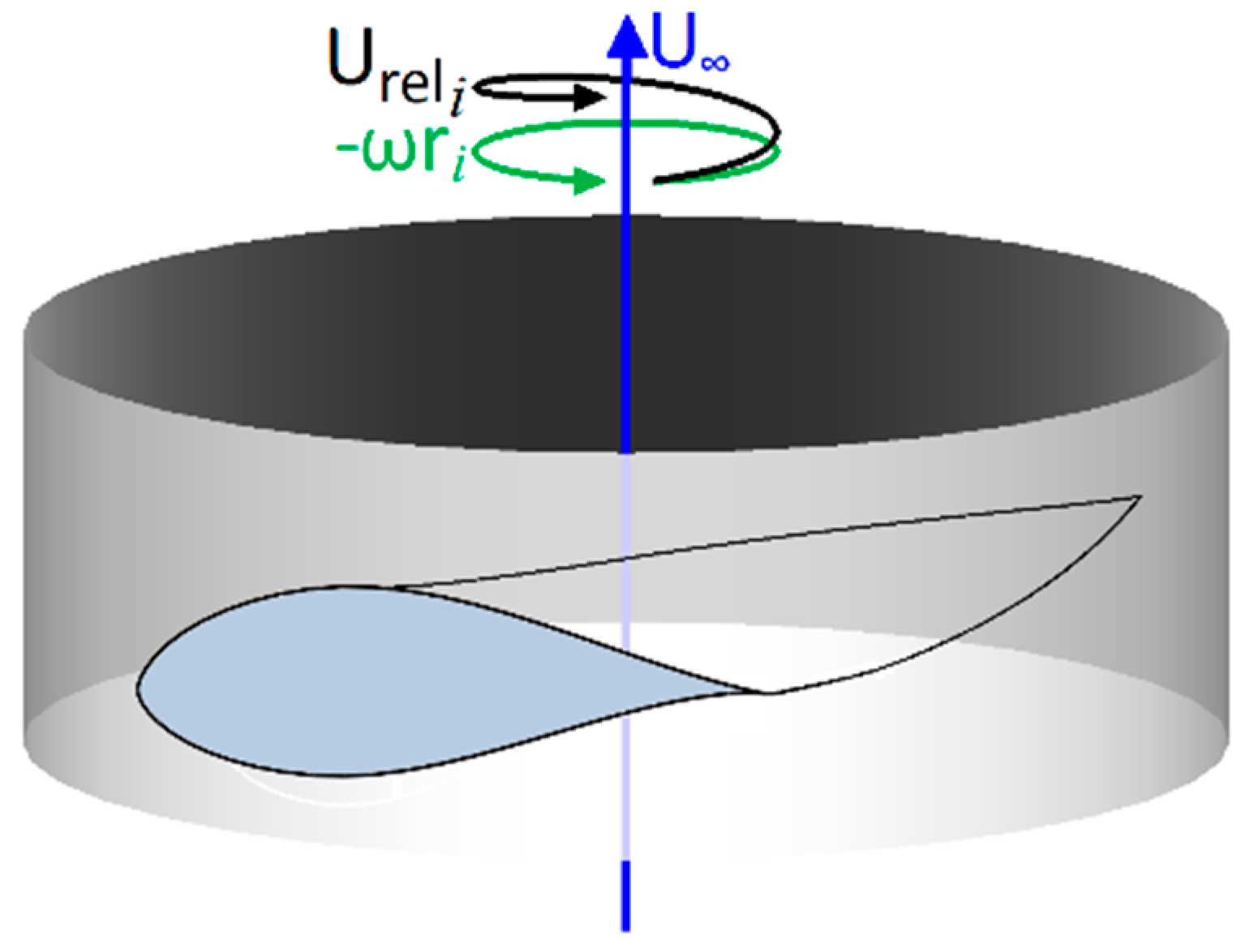
The separation points are determined via the 2D boundary layer analysis of Section 2.2, applied in the axial and tangential directions. The thick wake method then adopts the initial wake geometry illustrated in Figure 2, transformed to cylindrical coordinates, such that the undisturbed relative flow velocity is equal to the vector sum of the free stream velocity and the rotor’s local rotational velocity –ωri (Figure 3), and the wake length WL is a helical arc aligned with the relative flow. The wake shape, which is constrained in the ξ- (parallel with ) and η- (spanwise) directions, is then adjusted according to the local pressure values, Equation (6), by moving the ith wake panel vertex in the ζ-direction (perpendicular to ) from position to , as calculated by the nth iteration of the following Quasi-Newton method:
where is the difference between the pressure coefficients at the separation point and the ith wake panel. Convergence is achieved when all predicted pressure values in the separated wake are within 5% of the pressure at the separation point, which is typically very close to zero, such that a 5% tolerance along the separated wake corresponds to tolerances from as low as 0.1% to no more than 1% in terms of peak-to-trough pressure differentials.
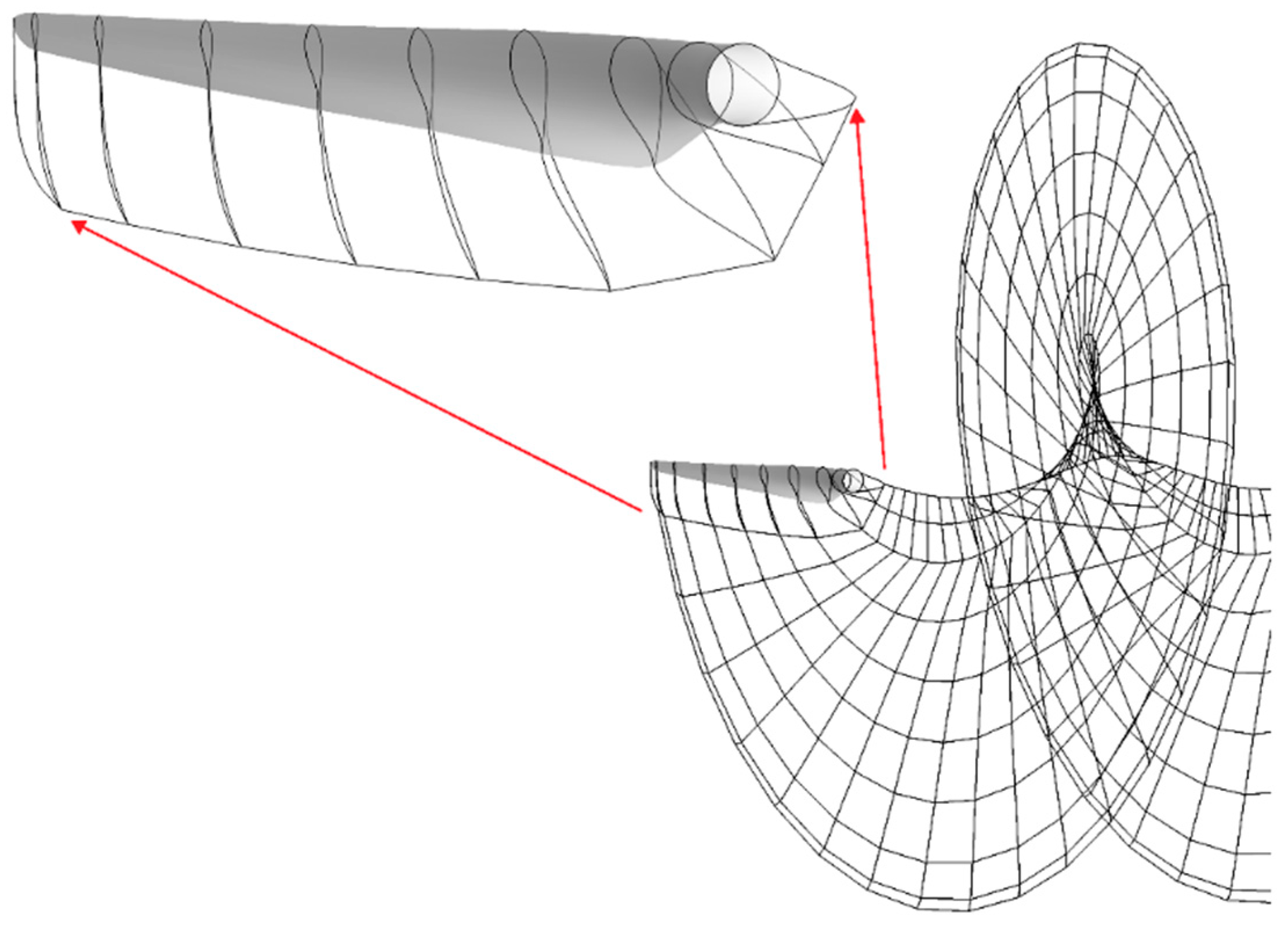
Finally, by treating the separated wake as an extension of the blade surface, the trailing edge of the “body” is now located at the intersection of the thick and thin wakes. (This separated wake “trailing edge” is visible in Figure 4, which also shows the separated “thick wakes”, as predicted by the current method, and helical thin wakes, aligned with the local flow, trailing behind several airfoil sections of one of the wind turbine’s rotor blades.) Manipulating the pressure around the “trailing edge” allows us to impose the Morino Kutta condition without having to implement an iterative pressure correction, as is common practice where strong 3D effects exist.
2.4. Viscous-Inviscid Coupling
The current method employs a very straightforward and intuitive method of coupling the inviscid and viscous solvers, by adopting the inviscid solution as an input for the viscous solver, and in turn incorporating a viscous correction, in this case a displacement of the inviscid surface streamline, back into the inviscid solver. However, these directly coupled models usually break down at separation due to the well-known Goldstein singularity, which is caused by a breakdown in the inviscid-viscous hierarchy, where the inviscid solution is no longer dominant.
Drela [33] overcame these hierarchal problems via computationally expensive merging of the viscous and inviscid equations into a large system of non-linear equations to be simultaneously solved by a global Newton-Raphson method. Veldman [34], to reduce this high computational cost, introduced the concept of an interaction law, which approximates the inviscid flow field. The interaction law and the viscous equations are solved simultaneously, and this solution is in turn input into the inviscid solver. Simultaneously coupled inviscid-viscous solvers, employing the “double wake” method, have more recently been applied to 2D yacht sails [35], unsteady pitching airfoils in stall conditions [36], and the quasi-3D (2D with rotational effects) analysis of rotating airfoils [37] and wind turbine rotors [38], while most of the recent work on the quasi-simultaneous approach has focused on deriving suitable interaction laws [39,40,41,42].
Notwithstanding the aforementioned convergence problems associated with direct coupling of the inviscid and viscous solvers, the current method was able to accurately simulate the severely separated flow around a rotating wind turbine rotor. “By modelling the separated wake as an extension of the displacement body, the thick wake model is able to avoid the Goldstein singularity, allowing for a fast, robust CFD tool, for which the computational expense of simultaneously solving the inviscid and boundary layer equations is no longer necessary” [6]. Furthermore, the speed and code-openness of the current method allow for ease of coupling for aeroelastic problems, optimisation algorithms, and actuator line models, all of which have recently found application in the modelling of full wind farms [43,44].
3. Results
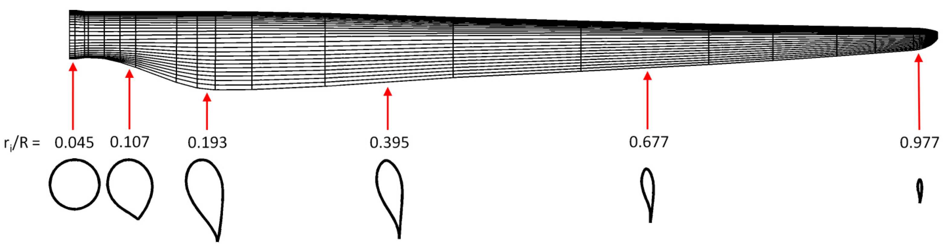
In order to assess the validity of the current method’s results, pressure distribution data was computed at a number of radial locations and compared with RANS predicted pressure data, solved in Fluent 6.2.16 via the SIMPLEC algorithm and one-equation Spalart-Allmaras turbulence model (a more detailed description of the model may be found in [22]), for a commercial 2 MW wind turbine rotor under normal operating conditions. Also included for comparison are 2D pressure data computed around identical airfoils in uniform flow using Xfoil [45], a 2D viscous-coupled panel method which is very popular for airfoil analysis, and is finding more use in wind turbine applications. The considered rotor blade is divided into a cylindrical section at the root, a transitional section, a so-called “aerodynamic” section, and a tip section. The rotor airfoil sections considered for analysis, as well as their non-dimensionalised radial locations and thickness-to-chord ratios, are summarised in Table 1 and Figure 5.
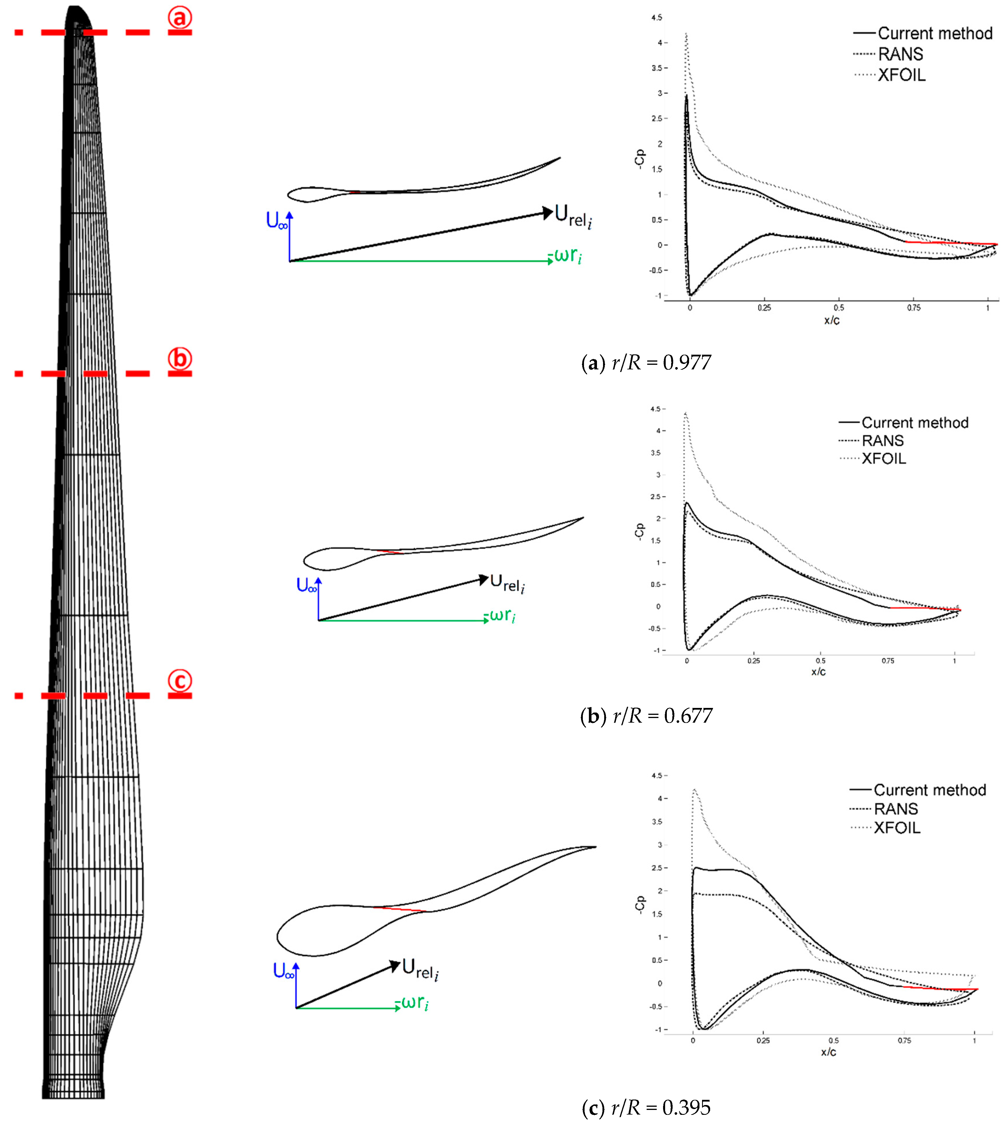
The combined airfoil-wake geometries, as predicted by the current method, are shown on the left hand side (LHS) of Figure 6, with the airfoils’ separation regions highlighted in red, and the undisturbed relative flow velocity vectors given as the vector sums of the free stream velocity and the rotor’s local rotational velocities −ωri. The right hand side (RHS) of Figure 6 shows the pressure data predicted by the current method, with the constant pressure distributions assumed to exist throughout the separation regions also highlighted in red, and the compared RANS and Xfoil data.
Along the outboard region of the rotor, namely at the rotor tip (Figure 6a) and at the outermost of the three considered “aerodynamic” sections (Figure 6b), the predicted separation regions extend over 26% of the suction surfaces, but the thickness of the separated wakes appears almost negligible. It is perhaps interesting to note that the orientation of the thick wake at these outboard sections appears to initially be more closely aligned with rotor’s plane of rotation, but, further downstream, is observed to veer away towards . The pressure data predicted by the current method show excellent agreement with the RANS data, with suction-side-minimum to pressure-side-maximum pressure differentials respectively 8% and 6% greater than those predicted by RANS, while Xfoil was found to significantly overpredict the suction peaks, with pressure differentials respectively 42% and 69% greater than those predicted by RANS.
At midspan (Figure 6c), the separation point was predicted to have advanced further towards the leading edge, with a predicted separation region of 31%. The separated wake is also noticeably thicker, and appears to undergo a slight undulation. The predicted pressure data at this section is slightly more conservative than that predicted by RANS, with a 19% greater pressure differential, while Xfoil’s predicted pressure differential exceeds that of the RANS data by 42%.
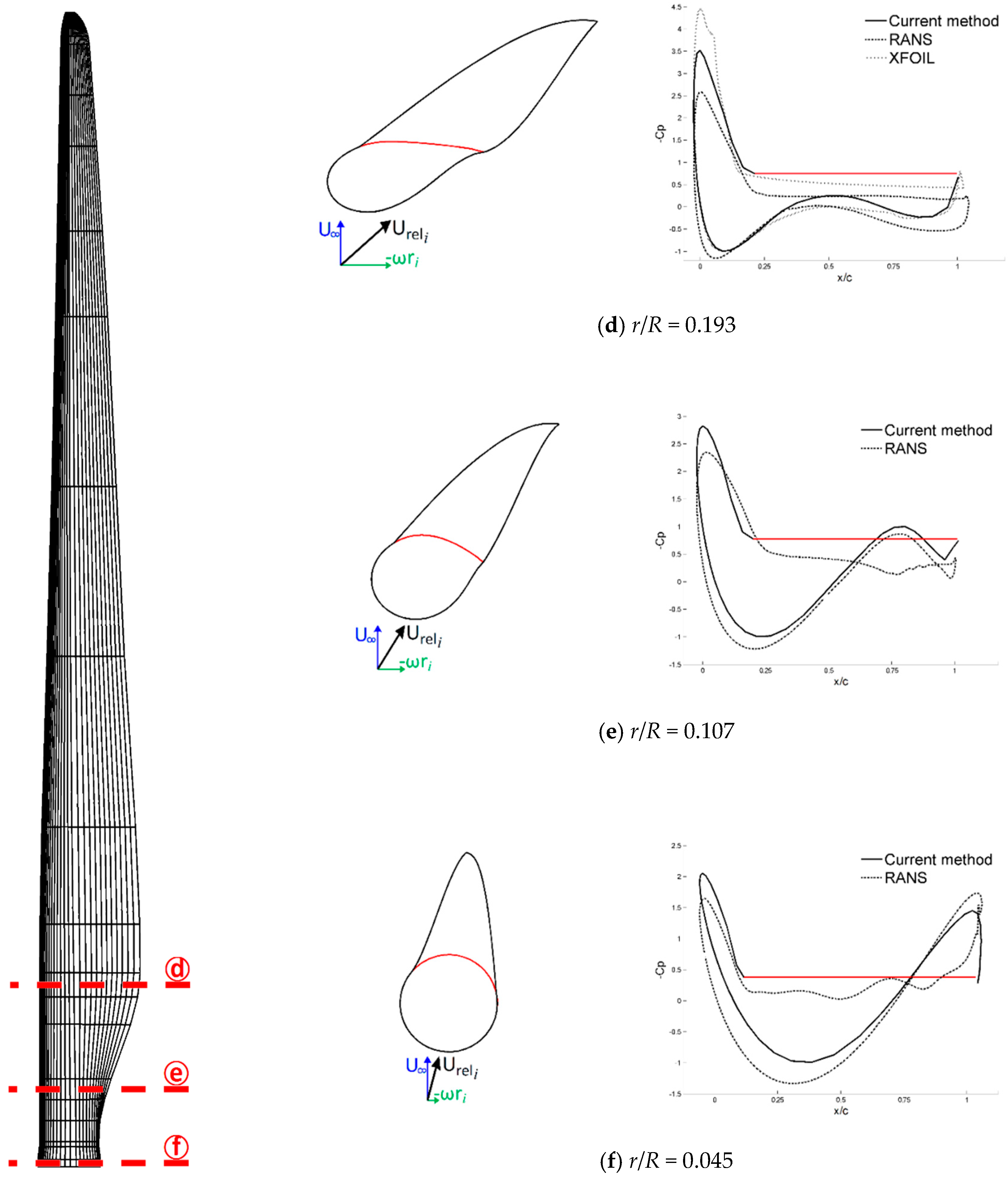
Finally, along the structural inboard region of the rotor, the flow has completely separated, with predicted separation regions at the innermost aerodynamic section (Figure 6d), transitional section (Figure 6e), and cylindrical section (Figure 6f) of 77%, 78.5%, and 84%, respectively, and an apparently proportional increase in the thickness of the separated wakes. At these inboard sections, the thick wakes appear to be well aligned with , although any variations in wake orientation are far less prominent due to the substantial thickness of the wakes. Despite the severe flow separation, the current method’s predicted pressure data is still highly comparable with the RANS data, with a slightly conservative 19% greater pressure differential at the innermost aerodynamic section, compared with Xfoil’s 46%, and just 4% and 2% greater pressure differentials at the transitional and cylindrical sections, respectively, at which Xfoil was unable to produce converged solutions.
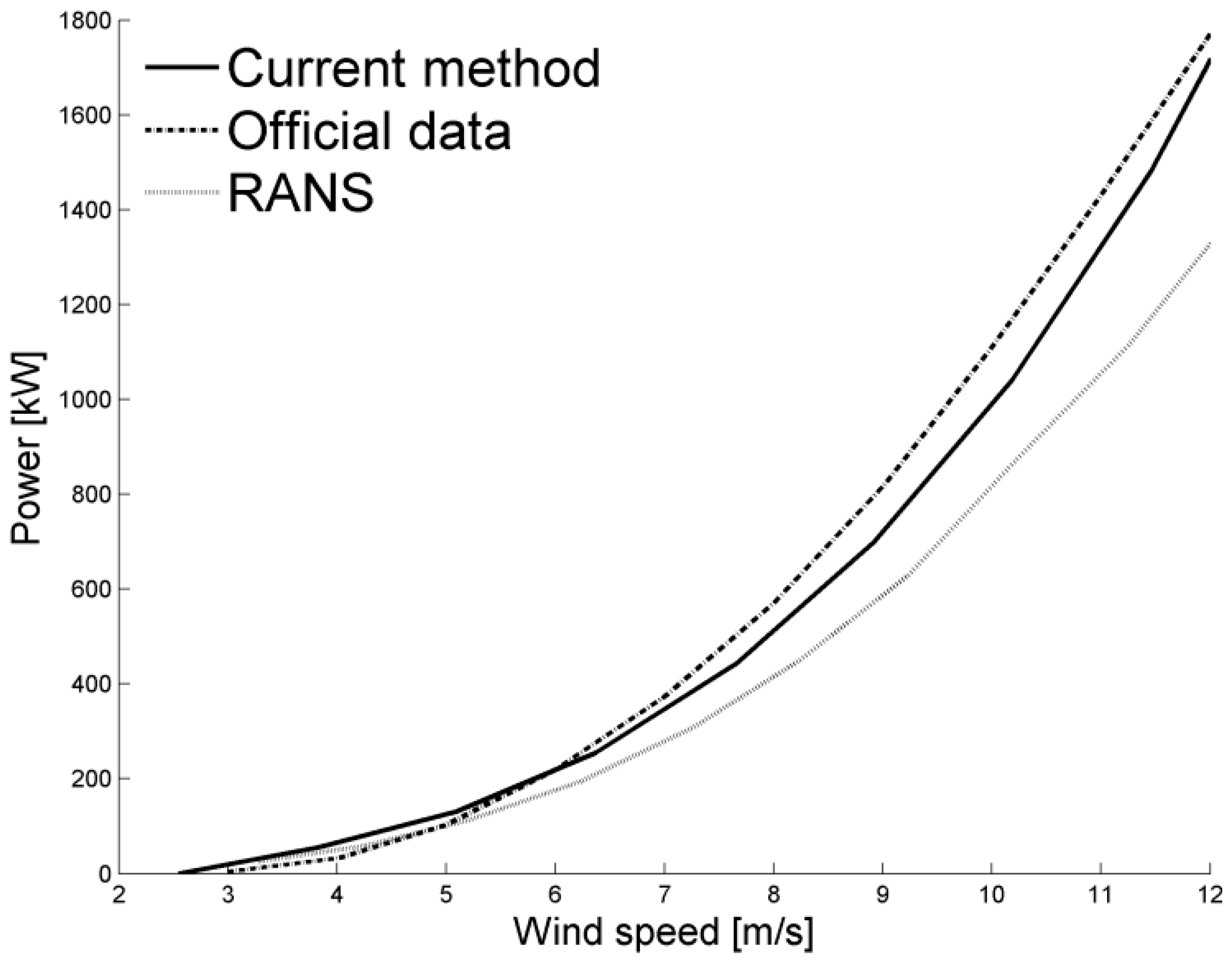
As an additional validation, the output power was computed for a range of wind speeds and wind turbine rotational speeds, from cut-in to nominal. (Nominal wind speed and rotational speed for the target turbine are, respectively, 13 m/s and 20 rpm. Due to a lack of data, a linear relationship was assumed between the wind speed and rotational speed.) The wind speed–power curve predicted by the current method was found to be more conservative than that predicted by the commercial RANS solver, but marginally lower than that provided by the turbine manufacturer, with just a 3% difference between output power at nominal wind speed and rotational speed, compared with the RANS solver’s 13% lower output power at the same conditions (See Figure 7 and Table 2).
4. Discussion
Along the outboard region of the wind turbine rotor, the rotor blade airfoils are better aligned with the undisturbed relative flow, and flow separation, although present to a lesser extent, does not significantly affect aerodynamic performance. The strong correlation between the current method and the RANS data in this flow-aligned region is thus not surprising. The significantly overpredicted data from the compared 2D panel method is most likely due to the inability of the method to account for tip losses; such 2D methods being restricted to the analysis of infinite wings in uniform flow.
Moving inward toward the root, however, ωri decreases with decreasing ri, as is clearly illustrated by the velocity vectors in Figure 6, resulting in higher angles of attack, and, consequently, more severe separation. Furthermore, the increased angles of attack combined with increased thickness-to-chord ratios result in a thicker separated wake, and, therefore, a more marked transition from displacement body streamline to separation streamline, which further exacerbates the adverse pressure gradient responsible for flow separation. The slight discrepancy between the pressure data predicted by the current method and that predicted by the RANS solver highlights the difficulty of numerically simulating a separated flow behind a rotating body. Of course, it is important to note that, despite a vast body of work on the accuracy and limitations of the RANS equations closed by appropriate turbulence models for the resolution of the turbulent boundary layer along wind turbine rotor blades, without corroborating experimental data, we cannot comment on the real-world accuracy of the compared RANS data, which therefore serve merely as code-to-code comparison. With this in mind, the current method’s predictions are considered highly satisfactory, especially in light of the substantial reduction in computational expense afforded by the current method, which employed around 2000 quadrilateral panels compared to the one million polyhedral cells employed by the RANS model.
Finally, along the inboard region of the rotor blade, aerodynamic efficiency has been sacrificed in favour of greater structural integrity, which has been achieved by very high thickness-to-chord ratios ranging from 0.4 at the innermost aerodynamic section to 1.0 at the cylindrical root section. Due to the combination of high thickness-to-chord ratios and supercritical angles of attack, the flow has completely separated from the suction surface of this section of the rotor blade. However, despite such severe flow separation, the current method’s predicted pressure data is still highly comparable with the RANS data, especially at the transitional and cylindrical sections. In addition to accuracy and speed, this also illustrates the robustness of the current panel method in modelling severely separated flows behind rotating bodies, considering that the compared 2D panel method was unable to produce converged results for these sections in uniform flow.
A brief comment on the predicted wind speed-power curve is that, due to a lack of data, the wind speed and rotational speed were assumed to have a linear relationship. This should explain the slight discrepancy between the power curve predicted by the current method and the official power data at sub-nominal wind speeds and rotational speeds. None the less, a maximum discrepancy between the two data sets of 11.6% at U = 9 m/s and a minimum discrepancy of just 3% at nominal conditions attest to the accuracy of the current method. On the other hand, the RANS data showed a maximum discrepancy 23% at U = 9 m/s and a minimum discrepancy of 13% at nominal conditions.
5. Conclusions
The flow field around a commercial 2 MW wind turbine rotor has been calculated using the proposed viscous-coupled 3D panel method. The validity of the results was assessed through code-to-code comparison with numerical data from a commercial RANS solver and a popular open-source 2D viscous-coupled panel method, as well as with data provided by the manufacturer. Along the outboard and inboard regions of the rotor, pressure data predicted by the current method show excellent agreement with the RANS data, while pressure data predicted along the midspan region were found to be slightly more conservative. The power curve predicted by the current method is also more conservative than that predicted by the commercial RANS solver, but lies just marginally below that provided by the turbine manufacturer, with just a 3% difference between output power at nominal wind speed and rotational speed, compared with the RANS solver’s 13% lower output power at the same conditions.
Taking into account the high degree of comparability with the more sophisticated RANS solver, the excellent agreement with the official wind turbine data, the considerably reduced computational expense afforded by the current method, which employed around 2000 quadrilateral panels compared to the one million polyhedral cells employed by the RANS model, not to mention the mesh generation and verification (watertightness and mesh independence testing) time saved by reducing the dimensionality of the discretisation, the author believes that this could be a powerful standalone tool for the design and analysis of wind turbine blades, or could be applied to the emerging field of wind farm layout design, by providing accurate body force input to actuator line rotors within full Navier-Stokes finite volume models of multi-unit wind farms.
Acknowledgments
This work was conducted in partial fulfillment of the requirements for the degree of Doctor of Philosophy. The author received no funding for this research.
Author Contributions
Bryan Nelson conceived and designed the study, and wrote the paper. Jen-Shiang Kouh is the author’s Ph.D. supervisor.
Conflicts of Interest
The authors declare no conflict of interest.
References
- Global Offshore Wind Speeds Rankings. 4C Offshore. Available online: www.4coffshore.com/windfarms/windspeeds.aspx (accessed on 26 January 2017).
- Taiwan Pledges EUR 2.5 Bln for 2020 OW Targets. Offshore WIND. Available online: www.offshorewind.biz (accessed on 26 January 2017).
- Chen, C.R.; Huang, W.P. On the precipitation monitoring and prediction of typhoon in Central Weather Bureau, Taiwan. In Proceedings of the 8th International Symposium on Social Management Systems—Disaster Prevention and Reconstruction Management, Kaohsiung, Taiwan, 2–5 May 2012. [Google Scholar]
- Typhoon Soudelor Causes Widespread Damage to Taiwan (Update). Focus Taiwan. Available online: focustaiwan.tw/news/asoc/201508090019.aspx (accessed on 26 January 2017).
- Vermeer, L.J.; Sørensen, J.N.; Crespo, A. Wind Turbine Wake Aerodynamics. Prog. Aerosp. Sci. 2003, 39, 467–510. Available online: http://www.sciencedirect.com (accessed on 5 February 2017). [CrossRef]
- Nelson, B.; Kouh, J.S. The numerical analysis of wind turbine airfoils at high angles of attack. Int. J. Energy Environ. Eng. 2016, 7, 1–12. Available online: http://link.springer.com/article/10.1007/s40095-015-0197-6 (accessed on 5 February 2017). [CrossRef]
- Sørensen, J.N.; Shen, W.Z. Numerical modeling of Wind Turbine Wakes. J. Fluids Eng. 2002, 124, 393–399. Available online: http://fluidsengineering.asmedigitalcollection.asme.org (accessed on 5 February 2017). [CrossRef]
- Mikkelsen, R.F. Actuator Disc Methods Applied to Wind Turbines. Ph.D. Thesis, Technical University of Denmark, Lyngby, Denmark, 2003. [Google Scholar]
- Panjwani, B.; Popescu, M.; Samseth, J.; Meese, E.; Mahmoudi, J. OffWindSolver: Wind farm design tool based on actuator line/actuator disk concept in OpenFoam architecture. In Proceedings of the First Symposium on OpenFOAM in Wind Energy, SOWE 2013, Oldenburg, Germany, 20–21 March 2013. [Google Scholar]
- Wilson, J.M.; Davis, C.J.; Venayagamoorthy, S.K.; Heyliger, P.R. Comparisons of Horizontal-Axis Wind Turbine Wake Interaction Models. J. Sol. Energy Eng. 2015, 137, 031001. [Google Scholar] [CrossRef]
- Troldborg, N. Actuator Line Modeling of Wind Turbine Wakes. Ph.D. Thesis, Technical University of Denmark, Lyngby, Denmark, 2008. [Google Scholar]
- Troldborg, N.; Sørensen, J.N.; Mikkelsen, R. Numerical Simulations of Wake Characteristics of a Wind Turbine in Uniform Flow. Wind Energy 2010, 13, 86–99. Available online: onlinelibrary.wiley.com (accessed on 5 February 2017). [CrossRef]
- Lu, H.; Porté-Agel, F. Large-Eddy Simulation of a Very Large Wind Farm in a Stable Atmospheric Boundary Layer. Phys. Fluids 2011, 23, 065101. [Google Scholar] [CrossRef]
- Martinez Tossas, L.A.; Leonardi, S. Wind Turbine Modeling for Computational Fluid Dynamics; NREL Technical Report SR-5000-55054; National Renewable Energy Laboratory: Golden, CO, USA, 2012. [Google Scholar]
- Churchfield, M.J.; Lee, S.; Michalakes, J.; Moriarty, P.J. A numerical study of the effects of atmospheric and wake turbulence on wind turbine dynamics. J. Turbul. 2012, 13, 1–32. Available online: www.tandfonline.com (accessed on 20 April 2017). [CrossRef]
- Churchfield, M.J.; Lee, S.; Moriarty, P.J.; Martinez, L.A.; Leonardi, S.; Vijayakumar, G.; Brasseur, J.G. A Large-Eddy Simulation of Wind-Plant Aerodynamics. In Proceedings of the 50th AIAA Aerospace Sciences Meeting including the New Horizons Forum and Aerospace Exposition, Nashville, TN, USA, 9–12 January 2012. [Google Scholar]
- Yang, X.; Boomsma, A.; Barone, M.; Sotiropoulos, F. Wind turbine wake interactions at field scale: An LES study of the SWiFT facility. J. Phys. Conf. Ser. 2014, 524. Available online: iopscience.iop.org/article/10.1088/1742-6596/75/1/012019 (accessed on 20 April 2017). [CrossRef]
- Dobrev, I.; Massouh, F.; Rapin, M. Actuator surface hybrid model. J. Phys. Conf. Ser. 2007, 75. Available online: iopscience.iop.org/article/10.1088/1742-6596/75/1/012019 (accessed on 8 February 2017). [CrossRef]
- Hess, J.L.; Smith, A.M.O. Calculation of Potential Flow about Arbitrary Bodies. Prog. Aerosp. Sci. 1966, 8, 1–138. [Google Scholar] [CrossRef]
- Filkovic, D. APAME Documentation. Graduate Work, University of Zagreb, Croatia. 2008. Available online: http://www.3dpanelmethod.com/documents/Graduate%20Work.pdf (accessed on 18 May 2007).
- Katz, J.; Plotkin, A. Low-Speed Aerodynamics; McGraw-Hill: New York, NY, USA, 1991; pp. 284, 287. [Google Scholar]
- Chen, Y.C. Numerical Study an Aerodynamics Effects of Gusting Winds on a Wind Turbine during Standstill. Master’s Thesis, National Taiwan University, Taipei, Taiwan, 2011. (In Traditional Chinese). [Google Scholar]
- Technical Description of the Z72 Wind Turbine; Zephyros: Hilversum, The Netherlands, 2004.
- Thwaites, B. Approximate Calculation of the Laminar Boundary Layer. Aeronaut. Q. 1949, 1, 245–280. Available online: www.cambridge.org/ (accessed on 8 February 2017). [CrossRef]
- Head, M.R. Entrainment in the Turbulent Boundary Layer; Technical Report; Aeronautical Research Council: London, UK, 1958. [Google Scholar]
- Cebeci, T.; Bradshaw, P. Momentum Transfer in Boundary Layers; Hemisphere: Washington, DC, USA, 1977. [Google Scholar]
- Wauquiez, C. Shape Optimization of Low Speed Airfoils Using MATLAB and Automatic Differentiation. Licentiate’s Thesis, Royal Institute of Technology, Stockholm, Sweden, 2000. [Google Scholar]
- Maskew, B.; Dvorak, F.A. The Prediction of Clmax Using a Separated Flow Model. J. Am. Helicopter Soc. 1977, 23, 2–8. [Google Scholar]
- Robinson, D.E. Implementation of a Separated Flow Panel Method for Wall Effects on Finite Swept Wings. Master’s Thesis, Massachusetts Institute of Technology, Cambridge, MA, USA, 1988. [Google Scholar]
- Rawlinson-Smith, R. Computational Study of Stalled Wind Turbine Rotor Performance. Ph.D. Thesis, Cranfield Institute of Technology, Cranfield, UK, 1991. [Google Scholar]
- Rao, B.M.; Dvorak, F.A; Maskew, B. An Analysis Method for Multi-Component Airfoils in Separated Flow; NASA Technical Report, NASA-CR-159300; NASA Langley Research Center: Hampton, VA, USA, 1980. [Google Scholar]
- García, N.R. Unsteady Viscous-Inviscid Interaction Technique for Wind Turbine Airfoils. Ph.D. Thesis, Technical University of Denmark, Lyngby, Denmark, 2011. [Google Scholar]
- Drela, M.; Giles, M.B. Viscous-Inviscid Analysis of Transonic and Low Reynolds Number Airfoils. AIAA J. 1987, 25, 1347–1355. Available online: www2.coe.pku.edu.cn (accessed on 8 February 2017). [CrossRef]
- Veldman, A.E.P. New quasi-simultaneous method to calculate interacting boundary layers. AIAA J. 1981, 19, 79–85. Available online: arc.aiaa.org (accessed on 8 February, 2017). [CrossRef]
- Veiga, A.E.L. The Analysis of Partially Separated Flow on Sail Systems Using a Sectional Method. Ph.D. Thesis, University of Southampton, Southampton, UK, 2006. [Google Scholar]
- Riziotis, V.A.; Voutsinas, S.G. Dynamic stall modelling on airfoils based on strong viscous-inviscid interaction coupling. Int. J. Numer. Meth. Fluids 2008, 56, 185–208. Available online: onlinelibrary.wiley.com (accessed on 8 February 2017). [CrossRef]
- García, N.R.; Sørensen, J.N.; Shen, W.Z. A strong viscous–inviscid interaction model for Rotating Airfoils. Wind Energy 2013, 17, 1957–1984. Available online: onlinelibrary.wiley.com (accessed on 8 February 2017). [CrossRef]
- García, N.R. Development of a Three-Dimensional Viscous-Inviscid Coupling Method for Wind Turbine Computations. In Proceedings of the ICOWES 2013, Lyngby, Denmark, 17–19 June 2013; pp. 69–81. [Google Scholar]
- Veldman, A.E.P. A simple interaction law for viscous–inviscid interaction. J. Eng. Math. 2009, 65, 367–383. Available online: link.springer.com/article/10.1007/s10665-009-9320-0 (accessed on 5 February 2017). [CrossRef]
- Bijleveld, H.A. Application of a Quasi-Simultaneous Interaction Method for the Prediction of Three-Dimensional Aerodynamic Flow over Wind Turbine Blades. Ph.D. Thesis, Rijksuniversiteit Groningen, Groningen, The Netherlands, 2013. [Google Scholar]
- Smith, L. An Interactive Boundary Layer Modelling Methodology for Aerodynamic Flows. MEng Thesis, University of Pretoria, Pretoria, South Africa, 2012. [Google Scholar]
- Sturdza, P.; Suzuki, Y.; Martins-Rivas, H.; Rodriguez, D. A Quasi-Simultaneous Interactive Boundary- Layer Model for a Cartesian Euler Solver. In Proceedings of the 50th AIAA Aerospace Sciences Meeting, Nashville, TN, USA, 9–12 January 2012. [Google Scholar]
- Sørensen, J.N. Aerodynamic Aspects of Wind Energy Conversion. Annu. Rev. Fluid Mech. 2011, 43, 427–448. Available online: http://www.ccpo.odu.edu/~klinck/Reprints/PDF/sorensenAnnRevFlMech11.pdf (accessed on 5 February 2017). [CrossRef]
- Larsen, G.C.; Réthoré, P.E. TOPFARM—A tool for wind farm optimization. In Proceedings of the 10th Deep Sea Offshore Wind R&D Conference, DeepWind’2013, Trondheim, Norway, 24–25 January 2013; Available online: http://www.sciencedirect.com/science/article/pii/S1876610213012708 (accessed on 5 February 2017). [CrossRef]
- Drela, M. XFOIL: An Analysis and Design System for Low Reynolds Number Airfoils. In Proceedings of the Conference on Low Reynolds Number Airfoil Aerodynamics, University of Notre Dame, Notre Dame, IN, USA, 16–18 June 1989. [Google Scholar]
Figure 1.
Wind turbine rotor with trailing helical wake, showing quadrilateral panels.

Figure 2.
Description of separated wake [6].
Figure 2.
Description of separated wake [6].

Figure 3.
Illustration of airfoil and separated wake in cylindrical coordinate system.

Figure 4.
Single rotor blade showing airfoil sections, separated “thick” wake, and helical thin wake, with “trailing edge” highlighted at root and tip.
Figure 4.
Single rotor blade showing airfoil sections, separated “thick” wake, and helical thin wake, with “trailing edge” highlighted at root and tip.

Figure 5.
Wind turbine rotor blade airfoil sections.

Figure 6.
Airfoil and wake geometries (LHS), and predicted −Cp distributions (RHS).


Figure 7.
Compared wind power curves.


Table 1.
Wind turbine rotor blade airfoil sections.
| Section Label | (f) | (e) | (d) | (c) | (b) | (a) |
|---|---|---|---|---|---|---|
| Section type | cylindrical | transitional | aerodynamic | aerodynamic | aerodynamic | tip |
| Radial location | ri/R = 0.045 | ri/R = 0.107 | ri/R = 0.193 | ri/R = 0.395 | ri/R = 0.677 | ri/R = 0.977 |
| Thickness/chord | ti/ci = 1.0 | ti/ci = 0.8 | ti/ci = 0.4 | ti/ci = 0.285 | ti/ci = 0.225 | ti/ci = 0.17 |
Table 2.
Wind power data.
| Velocity (m/s) | Power (kW) | Error (%) | |||
|---|---|---|---|---|---|
| Official Data | Current Method | RANS | |||
| 3 | 4 | 10 | 25 | 150.0 | 525.0 |
| 4 | 32 | 66 | 59 | 106.3 | 84.4 |
| 5 | 103 | 125 | 114 | 21.4 | 10.7 |
| 6 | 219 | 219 | 194 | 0.0 | -11.4 |
| 7 | 373 | 346 | 308 | −7.2 | −17.4 |
| 8 | 570 | 512 | 452 | −10.2 | −20.7 |
| 9 | 816 | 721 | 628 | −11.6 | −23.0 |
| 10 | 1110 | 991 | 879 | −10.7 | −20.8 |
| 11 | 1430 | 1323 | 1111 | −7.5 | −22.3 |
| 12 | 1770 | 1716 | 1539 | −3.1 | −13.1 |
© 2017 by the authors. Licensee MDPI, Basel, Switzerland. This article is an open access article distributed under the terms and conditions of the Creative Commons Attribution (CC BY) license (http://creativecommons.org/licenses/by/4.0/).
Share and Cite
MDPI and ACS Style
Nelson, B.; Kouh, J.-S. The Aerodynamic Analysis of a Rotating Wind Turbine by Viscous-Coupled 3D Panel Method. Appl. Sci. 2017, 7, 551. https://doi.org/10.3390/app7060551
AMA Style
Nelson B, Kouh J-S. The Aerodynamic Analysis of a Rotating Wind Turbine by Viscous-Coupled 3D Panel Method. Applied Sciences. 2017; 7(6):551. https://doi.org/10.3390/app7060551
Chicago/Turabian StyleNelson, Bryan, and Jen-Shiang Kouh. 2017. "The Aerodynamic Analysis of a Rotating Wind Turbine by Viscous-Coupled 3D Panel Method" Applied Sciences 7, no. 6: 551. https://doi.org/10.3390/app7060551
Note that from the first issue of 2016, this journal uses article numbers instead of page numbers. See further details here.