1. Introduction
To stay competitive, many companies all over the world try to go beyond the costly industry standard of preventative maintenance by implementing predictive maintenance procedures. For the industry related to oil exploitation, nuclear power and wind power, predictive maintenance procedures are the backbone in order to improve the operation and maintenance. Additionally, those industries for operation use drive trains that usually contain a gearbox as one of the key components. Vibration analysis is the most widely-used predictive maintenance procedure in gearbox predictive maintenance. In many mechanical systems, gearboxes are widely used for power transmission. Its condition is very important for the performance of the whole mechanical system. Therefore, many companies—and in the last two decades of academia also—have paid great attention to the gearbox condition monitoring. Vibration analysis can be applied very effectively to gearbox condition monitoring and predictive maintenance. In 2006, Jardine et al. [
1] reviewed the machinery fault diagnosis and prognosis in the condition-based maintenance view. The authors considered fault diagnosis as an important part of condition-based maintenance. We know that the gearbox is composed of many parts, such as gears, shafts, bearings, etc. In addition, there are many types of gearbox. The most typical are the fixed-axis gearbox and planetary gearbox. In 2011, bearing fault diagnosis work was reviewed by Randall and Antoni [
2]. Later, Ray and Upadhyay [
3] reviewed the signal processing techniques used in bearing fault diagnosis. This focuses mainly on the recent developments of the fault diagnosis signal processing techniques. Then, they discussed the advantages and disadvantages of these methods used in bearing fault diagnosis. For time-frequency analysis, Feng et al. [
4] reviewed more than 20 major time-frequency analysis methods used in fault diagnosis since 1990 and examined their advantages and disadvantages. As a major time-frequency analysis method, multiwavelet’s development in fault diagnosis has been reviewed by Sun et al. [
5]. Finally, they discussed the existing problems and future research directions. As we know, the fault mechanism of the planetary gearbox is very different from fixed-axis gearbox. Therefore, many authors pay great attention to the fault diagnosis of planetary gearboxes. Lei et al. [
6] reviewed the papers emerging in the planetary gearbox fault diagnosis domain and compared the fixed-axis and planetary gearbox fault diagnosis. Finally, they pointed to the potential research topics. Through these detailed review papers, readers will have a good knowledge of gearbox fault diagnosis.
Whether for the gear or the bearing, fault will produce impulse signals with a specific period. Therefore, the main object for fault diagnosis is to detect these impulse signals. Therefore, many methods were developed to detect impulse signals. Spectral kurtosis was one such effective method used for impulse signal detection. From its proposal, it becomes an important and effective way to detect the impulse signal. Recently, Wang et al. [
7] reviewed the development of spectral kurtosis and pointed out its future use in fault prognosis. Nevertheless, these periodic impulse signals (PIS) produced by fault are always overwhelmed by deterministic signals produced by the regular gear mesh and structural vibration. These deterministic signals are also called discrete frequency signals or the deterministic component. In order to detect the impulse signal more easily, it is necessary to suppress the deterministic signals. There are several methods developed to subtract the deterministic component from the original signal. The most dominant were: the autoregressive (AR) model method [
8,
9,
10,
11,
12,
13,
14,
15], time synchronous averaging [
16,
17,
18], adaptive noise cancellation [
19,
20] and the cepstrum pre-whitening method [
21,
22,
23]. These four methods all have been used in the separation of the deterministic signal and PIS signal successfully. Except for these methods, a new deterministic component cancellation method was proposed, recently [
24]. It is based on an iterative calculation of the signal envelope when the DC offset is cancelled before envelope calculation. The only parameter that needs to be pre-determined is the iteration number for DC offset cancellation. In the paper, a threshold of cross-correlation coefficient interval of [0.9, 0.95] was selected to judge the proper number of envelope calculations. The selected correlation coefficient interval was efficient for the examples in the paper, but this threshold method is not a proper way to acquire the most powerful PIS. Sometimes, a greater iteration number will distort the waveform of PIS and lead to the misdiagnosis of faults. In order to resolve this problem, correlated kurtosis (CK) is proposed to be used in determining when to stop the iteration for envelope calculation [
25]. This indicator can detect the PIS properly. However, CK is efficient only with strong enough PIS. When the PIS is very weak, CK is inefficient due to the inability to correctly detect the PIS. Therefore, in the case of very weak PIS, it is very difficult to determine the appropriate iteration number for envelope calculation.
Time frequency analysis methods, such as short time Fourier transform, the Wigner–Ville distribution and wavelet transform, were widely used in rotating machinery fault diagnosis. However, they all have some demerits. Compared to these time frequency analysis methods, the S transform can greatly avoid the existing deficiencies of the above three methods [
26]. Therefore, it can be used to display the time-frequency characteristics of the separation results of the deterministic component and the random component. In addition, fault features can be extracted from the resulting signal of the S transform to track the degradation of the component of interest. From the time-frequency contour produced by the S transform, one can distinguish the different faults more easily; or it can be used as the input for the deep learning methods to intelligent fault classification.
The above discussions show the need to use CK to optimize the iteration number of the envelope calculation with strong enough PIS. This can suppress the deterministic component effectively and properly. The S transform advantages inspire us to diagnose faults of the gearbox component by separation of the results of the deterministic component and the random component. The method is validated using the experimental datasets collected from a lab AC motor faulty bearing; a lab fixed-axis gearbox faulty bearing and gear and a lab planetary gearbox faulty sun, planet and ring gear. Experimental case studies will benefit the application of this novel method and will also provide a detailed guide for engineers in the industrial application. In addition, validation has been conducted using both intentionally-implanted bearing and gear damage data and naturally-developed distributed gear and bearing wear data under constant motor speed and various loads.
Based on the above-mentioned literature and analysis, the main contributions of this paper can be summarized as follows: (1) instead of the cross-correlation coefficient, correlated kurtosis was used as a criterion to estimate the optimal iteration number of DC offset cancellation, since CK has the superior ability to detect the PIS signal and is more robust to the noise interference; (2) when PIS is very weak compared with the deterministic signal or existing bearing fault and gear fault simultaneously, even CK cannot detect weak PIS produced by the bearing fault effectively; in this circumstance, the maximum order of high-speed shaft mesh frequency was used as the iteration number of DC offset cancellation; (3) because of several existing merits, the S transform was used to combine with DC offset cancellation to display the time-frequency characteristic of various gearbox faults; it is very efficient and intuitive to find faults through time-frequency contours; in addition, it could be used for deep learning-based fault classification; (4) through the planetary gearbox case study, it was found that DC offset cancellation is less effective for those small fault frequency signals, such as the planet gear, ring gear, carrier, etc.
Compared to the DC offset cancellation used in [
24], the advantage of this study is that it used CK instead of the cross-correlation coefficient to determine the optimal iteration number of DC offset cancellation. According to the CK’s value, it is more corrective to select the iteration number because it can detect PIS more accurately than the cross-correlation coefficient and is not easily interfered with by impulse-like noise. However, the disadvantage of this method is that it is less effective when the PIS is very weak. For the S transform, the advantages are that it can display the fault information more fruitfully and intuitively than the frequency domain. However, for some small fault frequencies, it is difficult to display them in the time-frequency contour because this needs a greater sampling length and will consume more computational resources, especially requiring a high ability graphic processing unit.
The remainder part of the paper is organized as follows. In
Section 2, a novel pre-whitening method and the S transform are briefly introduced. In
Section 3, the experimental case study of an implanted bearing outer race fault is presented. In
Section 4, the experimental case study of bearing and gear fault diagnosis in the gearbox is presented and explained in detail. In
Section 5, the experimental case study of the planetary gearbox fault diagnosis using the proposed method is presented. In
Section 6, the effectiveness and existing problem of the novel pre-whitening method are discussed. Finally,
Section 7 concludes the work.
3. Novel Proposed Method Application for Implanted Bearing Fault Diagnosis
The vibration fault dataset used in this case study was obtained from the Mechanical Failures Prevention Group (MFPT), assembled and prepared on behalf of MFPT by Eric Bechhoefer [
29]. Only the outer race faults are considered for evaluation and discussion in this research. The test bearings, which support the motor shaft, are radial ball bearings produced by RBC NICE with the following parameters: roller diameter 0.235 inch, pitch diameter 1.245 inch, number of elements 8 and the contact angle of 0°. In this case study dataset with a 25-Hz input shaft rate, a 48,828-Hz sampling frequency, a 3-s sampling duration and a 25-lbs. load are used. If we define the four bearing fault frequencies as ball pass frequency inner race (BPFI), ball pass frequency outer race (BPFO), ball spin frequency (BSF) and fundamental train frequency (FTF), fault frequencies could be calculated according to the geometric parameters [
30]. Four fault frequencies under the shaft rate of 25 Hz are: BPFO (81.12 Hz), BPFI (118.88 Hz), BSF (63.86 Hz) and FTF (10.14 Hz).
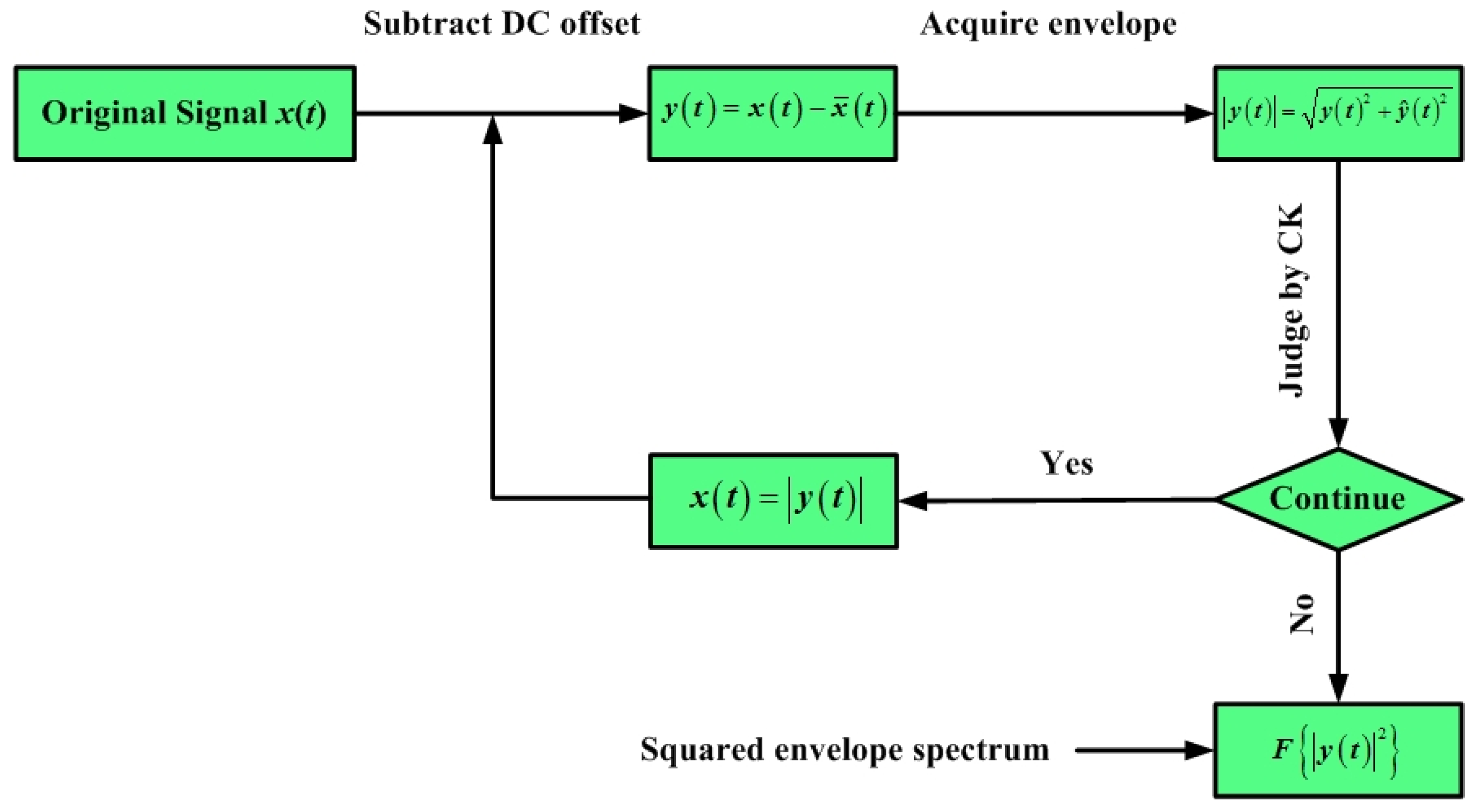
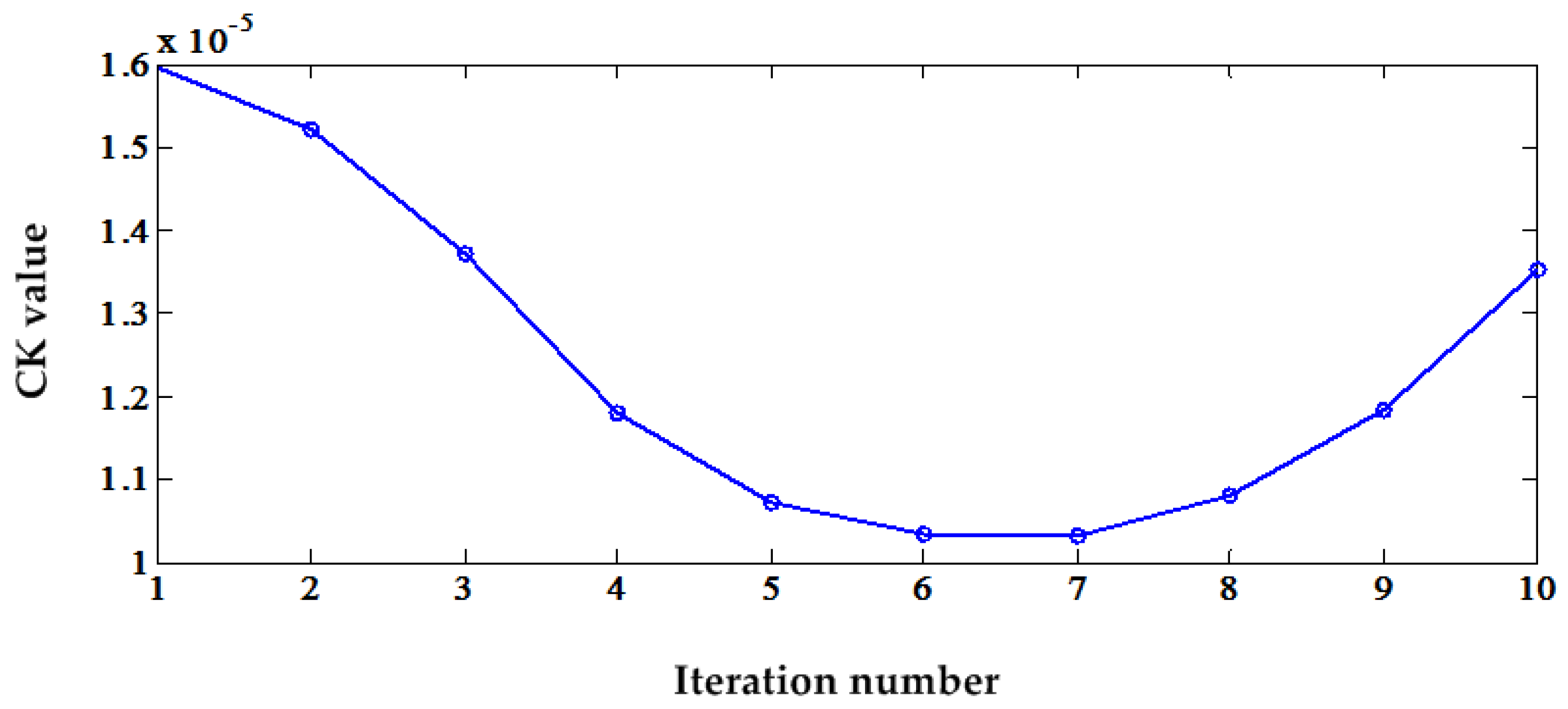
According to the framework in
Figure 1, the DC offset is gradually cancelled. First, the process is repeated 100 times, and CK and cross-correlated coefficient
μ are used to judge the termination of the iteration indicators. These two indicators, variation vs. iteration number, are illustrated in
Figure 2. The value of
μ increases, as can be seen, with the iteration number, but up to the 100th iteration. However, it cannot attain the threshold defined in [
24], which is [0.9, 0.95]. For the CK value, it increases at the beginning up to a high value, and then, it decreases. After the 15th iteration, it continues to increase. Two local optimal values were noticed during the 100 iteration process. Iteration 5 is the first one and the second one Iteration 85.
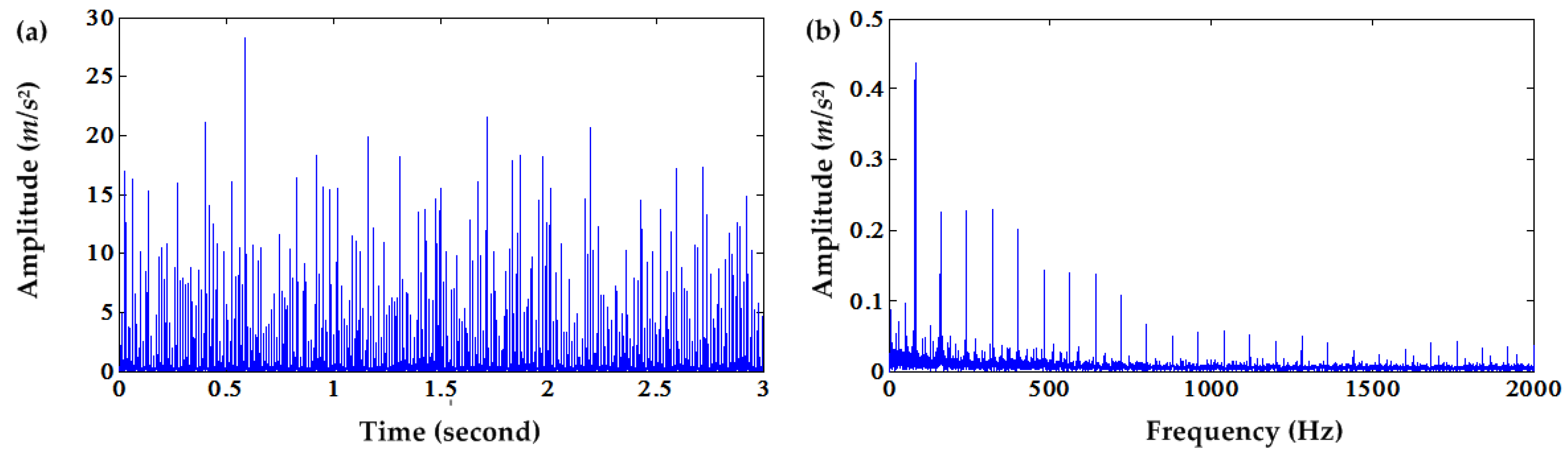
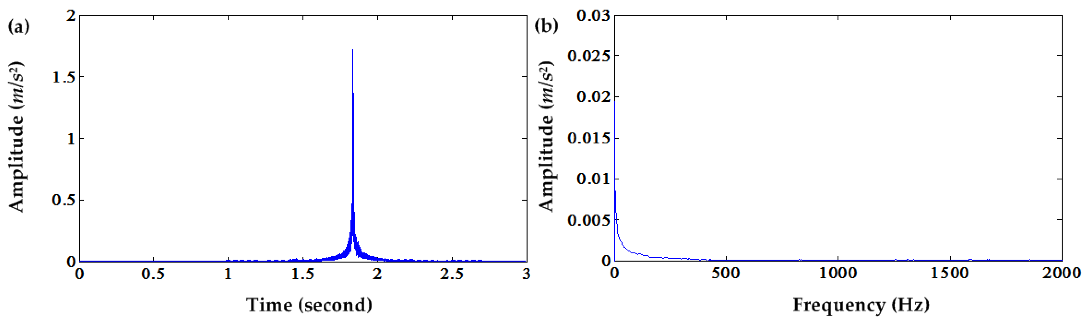
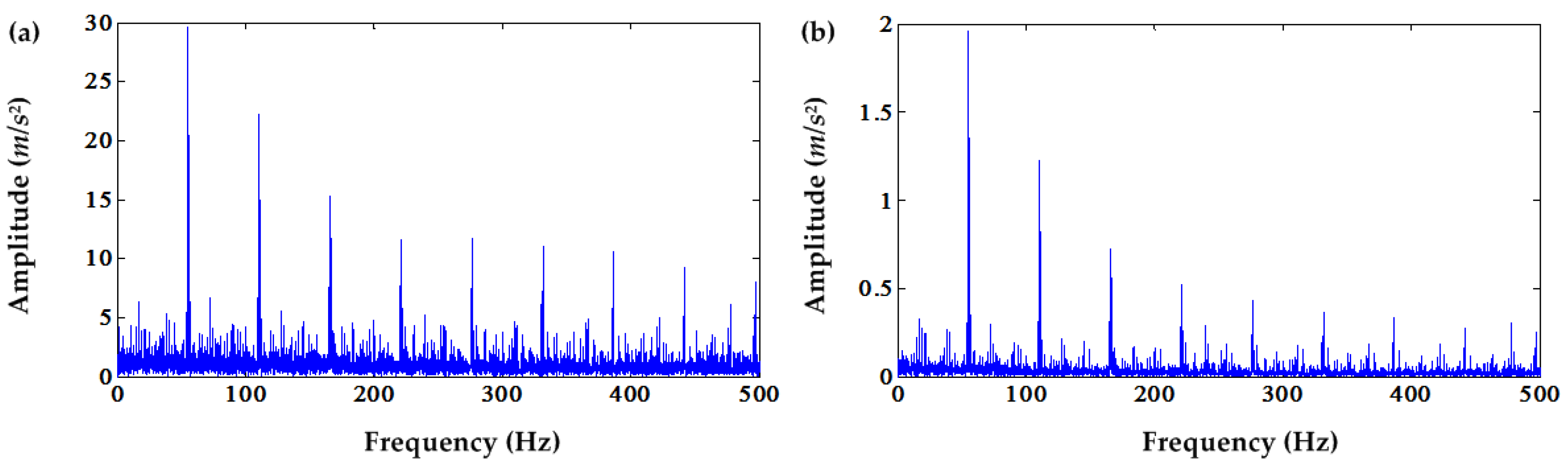
Figure 3 illustrates the squared envelope and its spectrum of the DC offset cancellation after the fifth iteration. The squared envelope and its spectrum of DC offset cancellation after the 100th iteration are shown in
Figure 4.
Figure 4 illustrates that normal envelope signals are distorted by an excess of DC offset cancellation. Moreover, the PIS of the squared envelope signal after the fifth DC offset cancellation is stronger than the original signal. Iteration 5 is the local optimum of the CK value. However, CK can detect the PIS signal when it is more intense than the other components. If the PIS are weak or not contained in the envelope signal, CK would not work, and its high value cannot denote the strong PIS. In this case, after the fifth iteration, the envelope signal is corrupted by excess DC offset cancellation operation. Actually, the CK values after the fifth iteration cannot denote the strength of PIS.
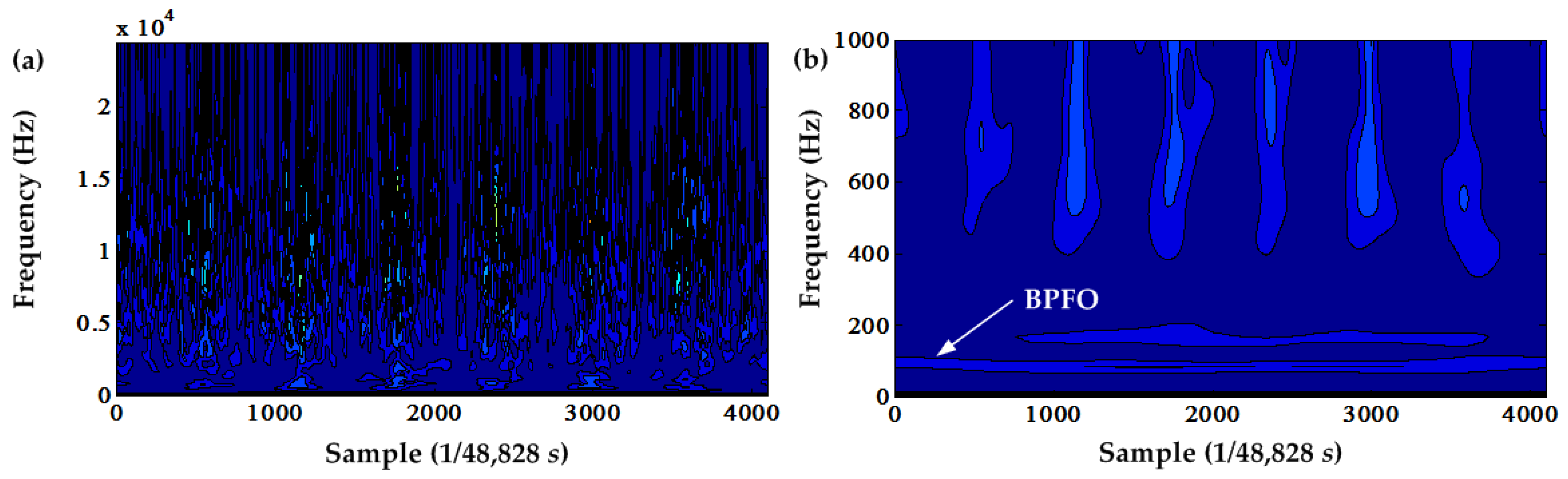
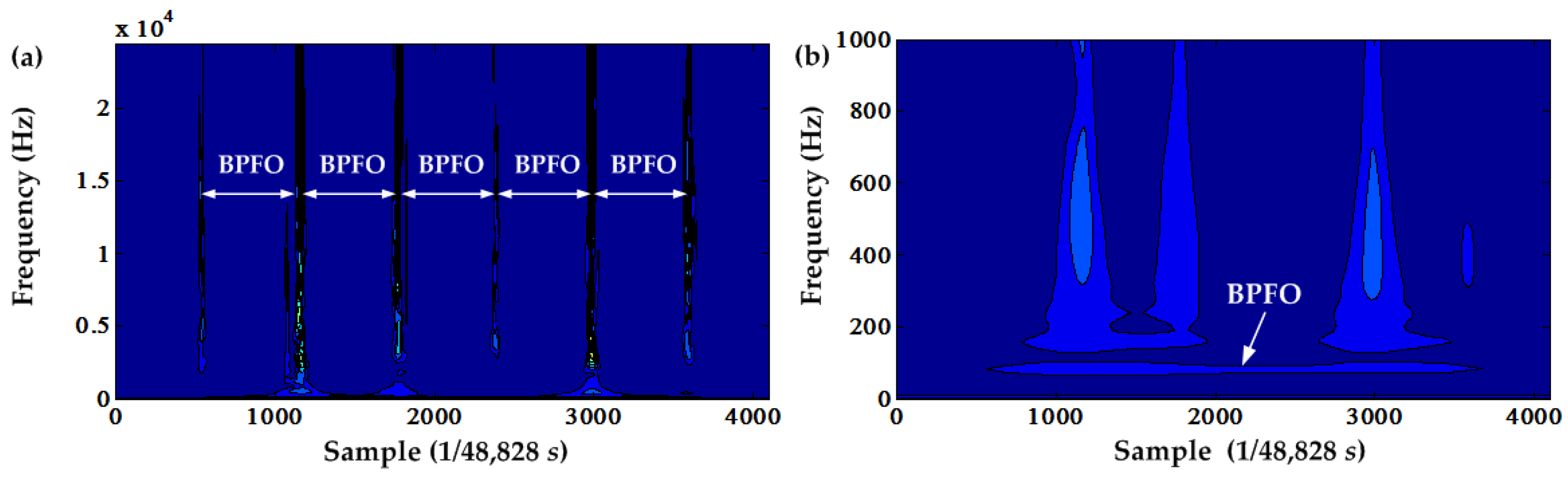
In order to observe the effect of DC offset cancellation from the time-frequency domain and compare it with the traditional envelope analysis, the S transform is applied to the squared envelope signal after the DC offset cancellation and the envelope signal of the original signal. The results are shown in
Figure 5 and
Figure 6. From the local amplification of these two time-frequency contours, the obvious BPFO can be seen in these figures. However, the time-frequency contour of the envelope of the original signal shown in
Figure 5a does not have an obvious BPFO contour, whereas the time-frequency contour of the squared envelope signal after the fifth DC offset cancellation has an obvious BPFO contour. This demonstrates that the DC offset cancellation suppresses the deterministic components and enables PIS clearly enough.
4. Novel Proposed Method Application for Naturally-Developed Fault Diagnosis
For the novel method application, experimental signals are collected from a lab fixed-axis gearbox test rig with naturally-developed bearing and gear faults. The dataset for testing high-speed (HS) shaft gear and bearings is from an end of life test case with an overall duration of 548 h. Detail end of life test case information can be found in [
31]. The intermediate speed (IS) shaft and its gears and bearings and the low speed (LS) shaft and its gear and bearings are from an ended implanted test case. Wear-in duration for the IS and LS shaft-related components lasted 10 h with different load and speed combinations.
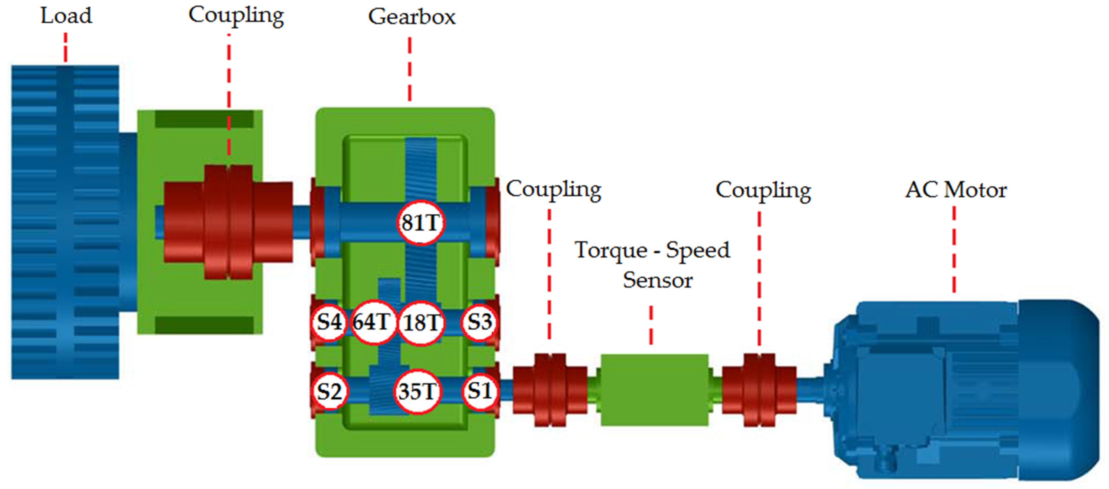
Figure 7 illustrates a schematic of the experimental gearbox test rig. It includes a two-stage fixed-axis gearbox, a 4-kW three-phase asynchronous motor for driving the gearbox and a magnetic powder brake for loading. The motor speed can be adjusted for different values. The NI data acquisition system consists of four IEPE accelerometers (Dytran 3056B4—Dytran Instruments Inc., Fraser, MN, USA), PXI-1031 mainframe, PXI-4472B data acquisition cards and LabVIEW software (National Instrument Inc., Austin, TX, USA). In addition, a tachometer and torque sensor is installed in the input shaft for acquiring the speed and load information. The internal structure of the gearbox is depicted in
Figure 7. The gearbox has three shafts supported by rolling element bearings. The LS shaft gear has 81 teeth and meshes with the IS shaft gear with 18 teeth. The IS shaft gear with 64 teeth meshes with the HS shaft with 35 teeth. Therefore, the overall gear ratio of the gearbox equals 8.22:1. In this case, study datasets with a 20-Hz input shaft rate, a 20-kHz sampling frequency, a 12-s sampling duration, a 199-Nm and 405-Nm loads are used.
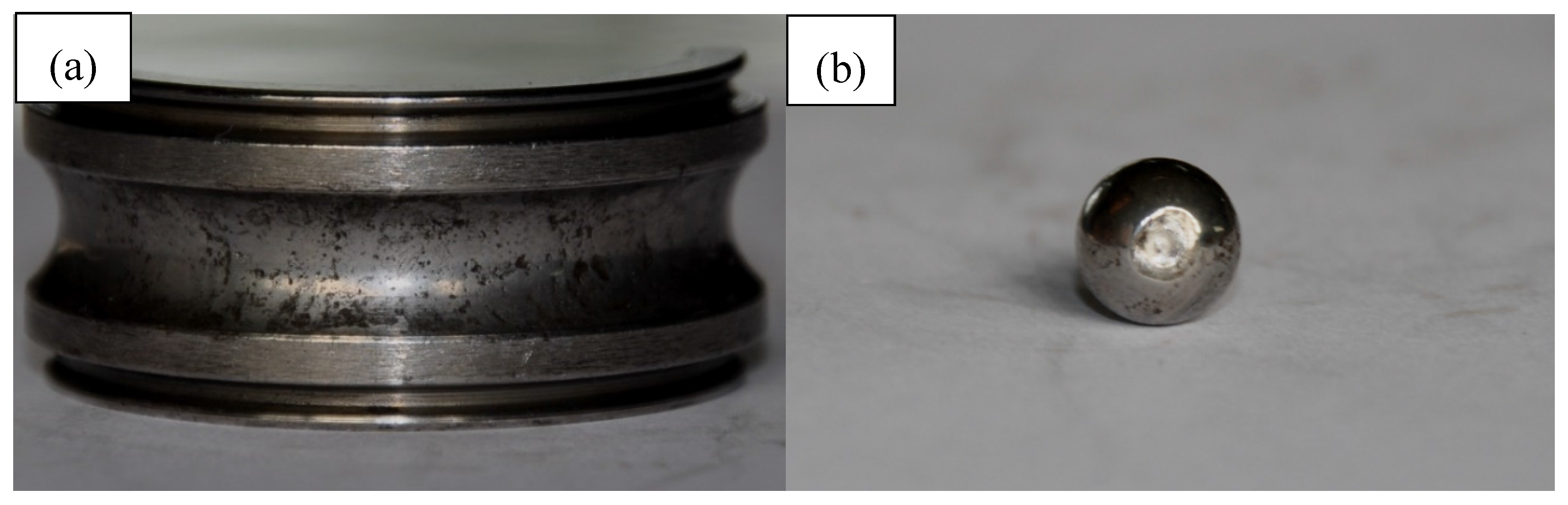
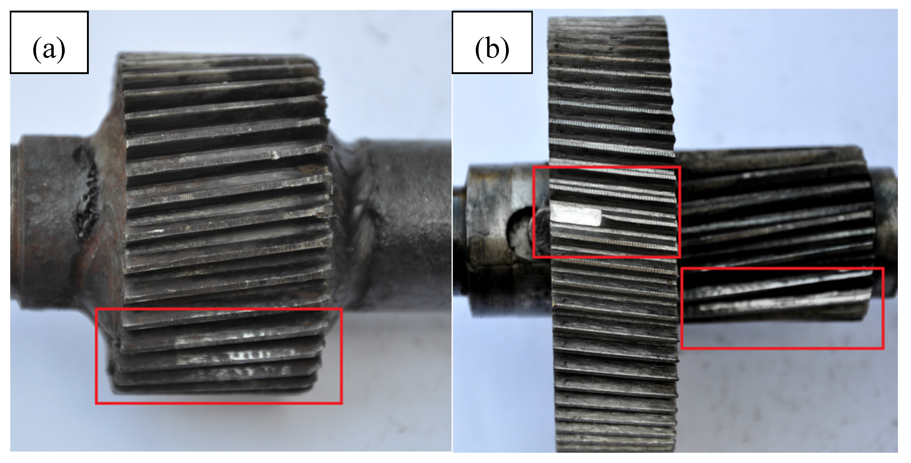
After the test, the gearbox was dismounted in order to check the bearings’ condition. It was found that all bearings have faults at different levels. However, only the HS shaft and LS shaft bearings have obvious faults. Both HS shaft bearings had the outer race fault shown in
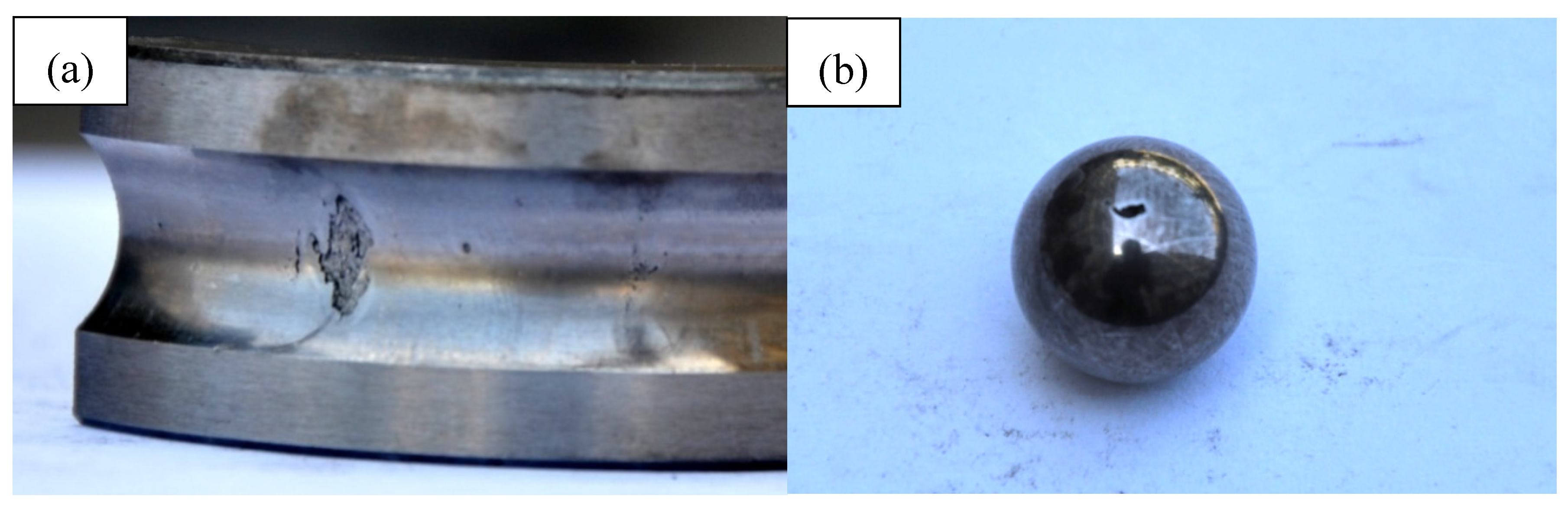
Figure 8a,b, and the right bearing in addition had the inner race fault and ball fault shown in
Figure 9a,b, respectively. Faults of the IS shaft bearing were not obvious faults. The left LS shaft bearing had the inner race fault and ball fault shown in
Figure 10a,b, respectively. The HS and IS shaft are supported by SKF 6205 bearings and the LS shaft by SKF 6208 bearings. The fundamental faults frequencies of SKF 6205 under a 1-Hz rotating speed are BPFO (3.585 Hz), BPFI (5.415 Hz), BSF (2.357 Hz) and FTF (0.398 Hz). For SKF 6208, they are BPFO (3.578 Hz), BPFI (5.423 Hz), BSF (2.337 Hz) and FTF (0.398 Hz). Therefore, the actual fault frequencies can be acquired through these fundamental frequencies multiplied by the rotating frequency. The bearing types and the characteristic frequencies for a 20-Hz input shaft rate are concerned and summarized in
Table 1.
It is very difficult to diagnose the bearing fault of the LS shaft because of the low speed and requirement of special techniques. In this case, only HS bearing faults under loads of 199 Nm and 405 Nm are considered. Except the bearing faults, the HS shaft gear with 35 teeth had a slight tooth wear fault. The IS shaft gear with 64 teeth had a chipped tooth fault, and the IS shaft gear with 18 teeth had a severe tooth wear fault shown in
Figure 11. For a gear transmission with fixed axes, the gear meshing frequency (GMF) can be calculated by the following formula: GMF =
N ×
Z, where
N means the rotating speed of the test gear and
Z represents the number of the test teeth. According to this, the GMF of the HS and IS shaft gears is determined as 700 Hz, and the GMF of the IS and LS shaft gears is determined as 196.93 Hz.
First, in order to ensure stable signal, the data acquisition system is adjusted to use the data sample rate based on the tachometer signal. The adjusted sampling rate is a synchronous sampling rate and donates the resampled vibration signal. During the experiment, the load of 199 Nm was applied to the output shaft (LS shaft), and the resampled signal is used. An accelerometer was mounted on the top of the gearbox casing (as shown in
Figure 7), and the vibration signals were collected from the accelerometer at position S2.
Figure 12a illustrates the correlation coefficient variation vs. the iteration number of DC offset cancellation, while
Figure 12b illustrates the CK value variation vs. the iteration number of DC offset cancellation.
Figure 12c illustrates the squared envelope signal after the 100th iteration. It can be seen that both the correlation coefficient and CK cannot be used to determine the optimal iteration number for DC offset cancellation in the multi-fault mode case. Especially for the weak PIS, CK will not work. However, as mentioned in
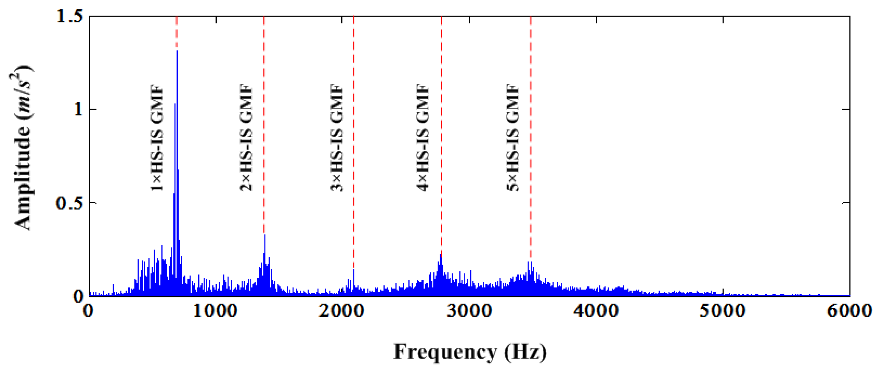
Section 2.1, one DC offset cancellation operation can subtract one harmonic deterministic component. In this case, HS shaft gear mesh frequency and its harmonics dominate the frequency spectrum, as shown in
Figure 13. It can be seen that there are mainly five harmonics of the gear mesh frequency. Therefore, theoretically, only five-times DC offset cancellation can suppress the deterministic component of the original signal. Therefore, we conduct five iteration DC offset cancellation for the time synchronous signal. The squared envelope spectrum and its time-frequency contour are illustrated in
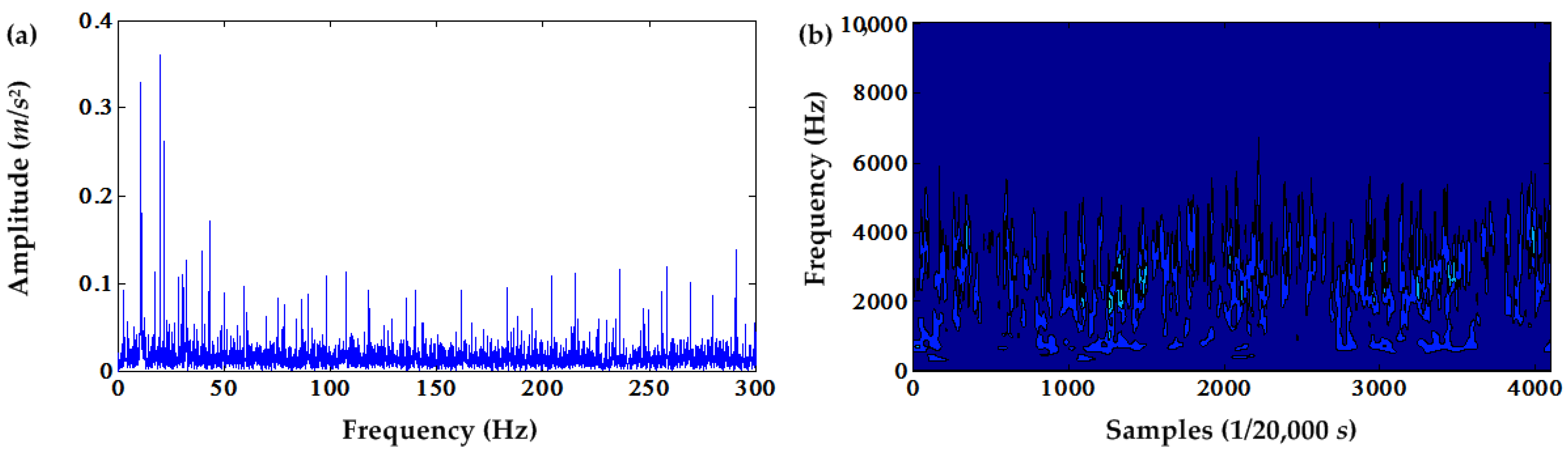
Figure 14. After checking the squared envelope spectrum carefully, it is very hard to find the bearing fault frequencies. Instead of the bearing fault frequencies, the squared envelope spectrum is dominated by the HS and IS shaft rate and its harmonics because of the gear chip fault and wear fault. However, in the time-frequency contour of the squared envelope signal, weak BPFO, BPFI and BSF information can be seen. On the contrary, no bearing fault information from the envelope spectrum and time-frequency contour of the original signal shown in
Figure 15 can be seen. Similarly, the envelope spectrum of the original signal is also dominated by the HS and IS shaft rate and its harmonics.
Second, in order to ensure a stable signal, the data acquisition system is adjusted to use the data sample rate based on the tachometer signal. The adjusted sampling rate is a synchronous sampling rate and donates the resampled vibration signal. During the experiment, the load of 405 Nm was applied to the output shaft (LS shaft), and resampled signal is used. An accelerometer was mounted on the top of the gearbox casing (as shown in
Figure 7), and the vibration signals were collected from the accelerometer at position S2.
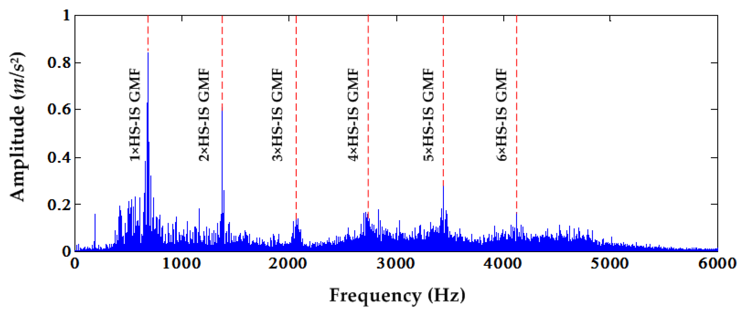
Figure 16 illustrates the frequency spectrum of the time synchronous signal with the dominant six harmonics of the HS-IS GMF. Therefore, for the DC offset cancellation operation, we can repeat six times to delete the deterministic component. Finally, the squared envelope spectrum and relevant time-frequency contour can be acquired as shown in
Figure 17. Similarly, the squared envelope spectrum is dominated by the HS and IS shaft rate and its harmonics. Information about the bearing fault frequencies cannot be found in the squared envelope spectrum. However, weak BPFI and BSF can be found in the time-frequency contour by the S transform. In order to compare with the traditional envelope analysis, the envelope spectrum of the time synchronous signal is given in
Figure 18a. The time-frequency contour of the envelope signal of the time synchronous signal is illustrated in
Figure 18b. It can be seen that it is very difficult to find any bearing fault-related information from this time-frequency contour.
5. Novel Proposed Method Application for Planetary Gearbox Fault Diagnosis
In this section, for the novel method application, experimental signals are collected from a lab planetary gearbox test rig with implanted wear tooth faults on the sun, planet and ring gear.
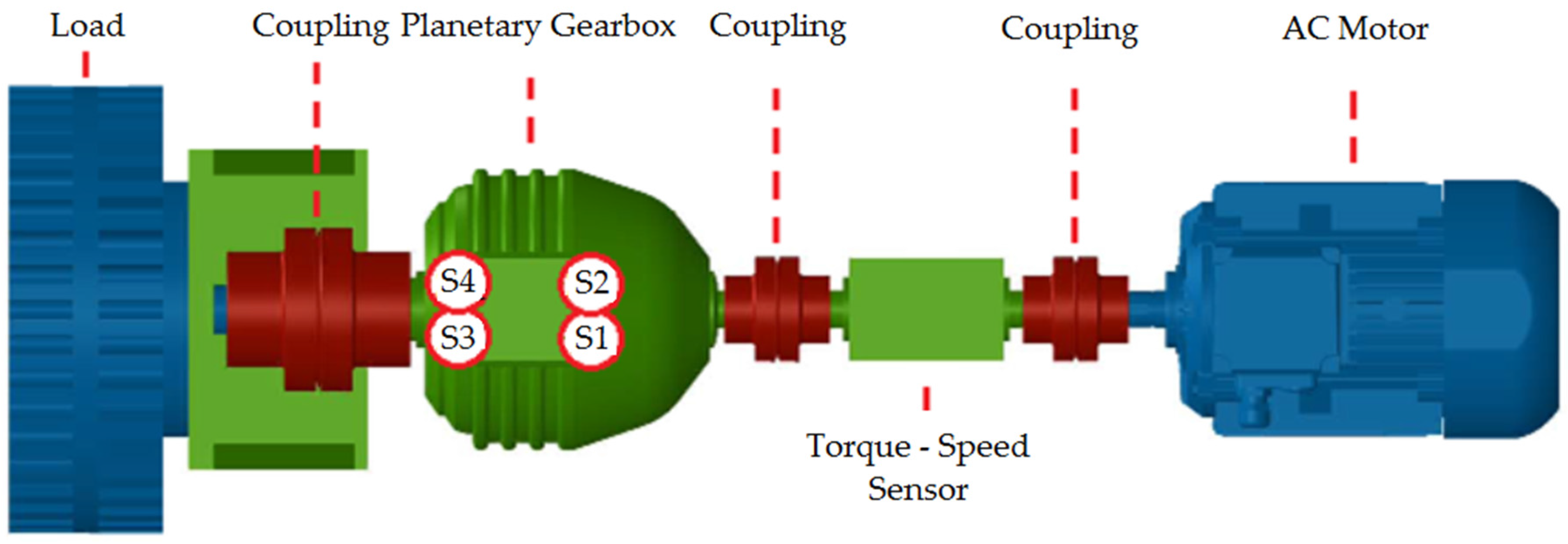
Figure 19 illustrates a schematic of the experimental planetary gearbox test rig. It includes a single-stage planetary gearbox, a 4-kW three-phase asynchronous motor for driving the gearbox and a magnetic powder brake for loading. The motor speed can be adjusted for different values. The load can be adjusted by a brake controller through the current of the magnetic powder brake connected to the output shaft (carrier). The NI data acquisition system consists of four IEPE accelerometers (Dytran 3056B4, Dytran Instruments Inc., Fraser, MN, USA), PXI-1031 mainframe, PXI-4472B data acquisition cards and LabVIEW software (National Instrument Inc., Austin, TX, USA). In addition, a tachometer and torque sensor is installed in the input shaft for acquiring the speed and load information. The single-stage planetary gearbox consists of the sun gear, planet gear and fixed ring gear. The sun gear is connected to the input shaft and rotates around its own center. All planet gears mesh simultaneously with the sun gear and ring gear. These planet gears not only rotate around their own centers, but also revolve around the center of the sun gear, and vibration signals picked up by a fixed sensor attached to the planetary gearbox housing differ significantly from that of fixed-axis/parallel gear systems [
32]. Compared to the fixed-axis gearbox test rig in
Section 4, all of the settings are the same, except the gearbox type. Single-stage planetary gearbox gear parameters are listed in
Table 2.
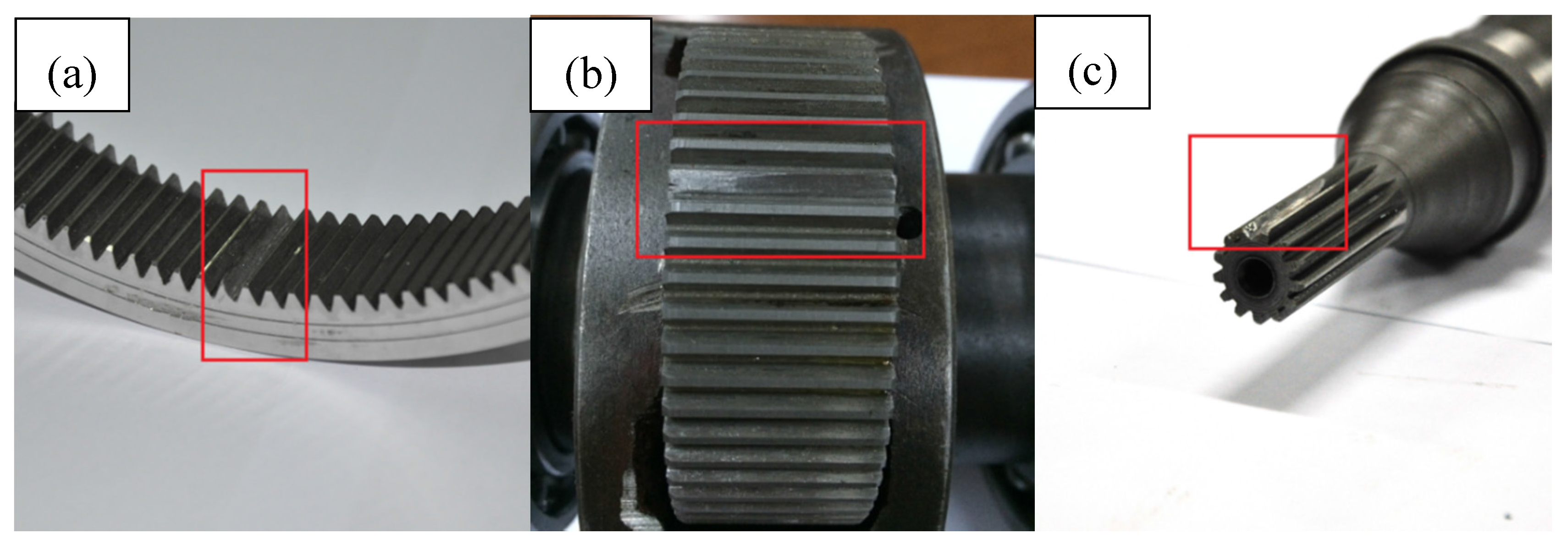
Wear gear faults of the planetary gearbox were implanted in one tooth of the ring gear, planet gear and sun gear, respectively, in order to validate the proposed analysis method.
Figure 20 illustrates the implanted gear faults.
Tooth wear faults belong to localized fault, and their fault frequencies can be calculated through the following equations [
33]. The meshing frequency for the stationary ring gear
fmesh =
fcarrier ×
Zring equals the product of the planet carrier rotating frequency
fcarrier and the number of ring gear teeth
Zring. Relative rotating frequency with respect to the planet carrier is
frelative =
fmesh/
Z, where
Z is the total number of teeth of the gear of interest. The characteristic frequency of faulty planet gear is
fplanet1 =
fmesh/
Zplanet, where
Zplanet is the number of planet gear teeth. If the damage exists on both sides of the gear tooth, the damaged planet gear tooth also meshes with the other mating gear. The characteristic frequency of the faulty planet gear becomes
fplanet2 = 2 ×
fmesh/
Zplanet. The characteristic frequency of the faulty sun gear equals the relative rotating frequency of the sun gear multiplied by the number of planet gears
fsun =
Nplanet ×
fmesh/
Zsun, where
Zsun is the number of sun gear teeth and
Nplanet is the number of planet gears. The characteristic frequency of the faulty ring gear is
fring =
Nplanet ×
fmesh/
Zring. Similarly, for the distributed damage case, the characteristic frequency of the faulty ring gear is
fring =
fmesh/
Zring.
5.1. Sun Gear Fault Experiment
For this experiment, we used a sun gear wear fault mode to test the proposed method while the remaining gears were all in good condition, undamaged. Similar to the case study in
Section 4, in order to ensure a stable signal, the data acquisition system is adjusted to use the data sample rate based on the tachometer signal. The adjusted sampling rate is a synchronous sampling rate and donates the resampled vibration signal. During the experiment, the mean rotating frequency of the input shaft connecting the sun gear of the planetary gearbox was 20.0889 Hz, while a load of 405 Nm was applied to the output shaft connecting the planet carrier. An accelerometer was mounted on the top of the gearbox casing (as shown in
Figure 19), and the vibration signals were collected from the accelerometer at position S3. According to the planetary gearbox configuration and its running speed, the characteristic frequencies are calculated and listed in
Table 3.
According to the framework of the proposed method, the squared envelope signal after DC offset cancellation is acquired. For this case, the CK value shows that the first envelope has the biggest PIS, as shown in
Figure 21. The squared envelope spectrum after the first DC offset cancellation and the envelope spectrum of only the time synchronous signal are illustrated in
Figure 22. Compared to the envelope spectrum of the original signal, the amplitudes of the sun gear fault frequency and its harmonics are much higher compared to the envelope spectrum of the original signal. However, it can also be noticed that the noise amplitudes unrelated to the sun gear fault frequency are also higher compared to the envelope spectrum of the original signal.
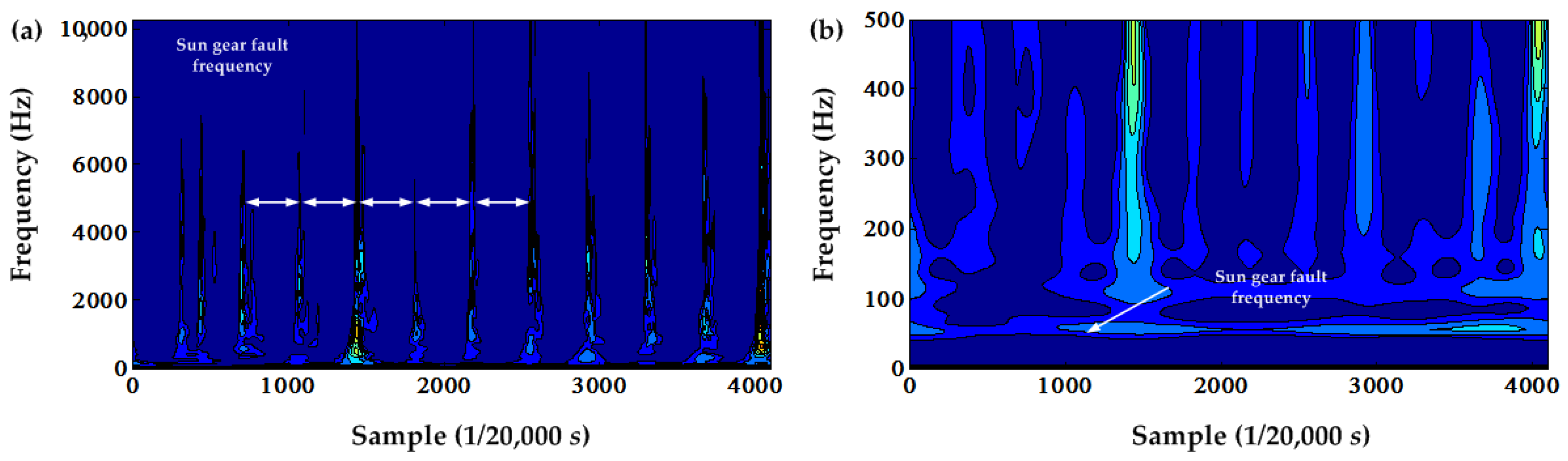
The time-frequency contour of the squared envelope signal using the S transform is shown in
Figure 23. In contrast, the time-frequency contour of the original envelope signal using the S transform is shown in
Figure 24. From these two figures and their local amplifications, the sun gear fault frequency in the frequency domain and the time-frequency domain can be seen. However, the time-frequency contour of the squared envelope signal has less useful sun gear fault information than the time-frequency contour of the original envelope signal.
5.2. Planet Gear Fault Experiment
For this experiment, we analyzed one planet gear wear fault mode to test the proposed method while the remaining gears were all in good condition, undamaged. Similar to the case study in
Section 4, in order to ensure a stable signal, the data acquisition system is adjusted to use the data sample rate based on the tachometer signal. The adjusted sampling rate is a synchronous sampling rate and donates the resampled vibration signal. During the experiment, the mean rotating frequency of the input shaft connecting the sun gear of the planetary gearbox was 20.0111Hz, while a load of 405 Nm was applied to the output shaft connecting the planet carrier. An accelerometer was mounted on the top of the gearbox casing (as shown in
Figure 19), and the vibration signals were collected from the accelerometer at position S3. According to the planetary gearbox configuration and its running speed, the characteristic frequencies are calculated and listed in
Table 4.
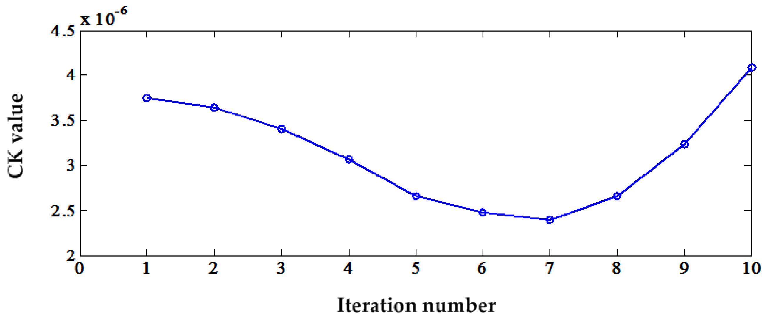
Similarly, we can apply the DC offset cancellation operation to this signal. The CK value shows that the signal only after the first DC offset cancellation iteration has the strongest PIS. The CK value variation vs. the iteration number can be seen in
Figure 25. Though the CK achieves highest value at the 10th iteration, after Iteration 6, the envelope signal is corrupted seriously. Therefore, the first iteration is optimal. The comparison of the squared envelope spectrum and original envelope spectrum is shown in
Figure 26. It can be seen that there is no difference in essence, except the amplitude. Because of the very small planet gear fault frequencies, it is very difficult to display the time-frequency contour using the S transform.
5.3. Ring Gear Fault Experiment
For this experiment, we used a ring gear wear fault mode to test the proposed method while the remaining gears were all in good condition, undamaged. Similar to the case study in
Section 4, in order to ensure a stable signal, the data acquisition system is adjusted to use the data sample rate based on the tachometer signal. The adjusted sampling rate is a synchronous sampling rate and donates the resampled vibration signal. During the experiment, the mean rotating frequency of the input shaft connecting the sun gear of the planetary gearbox was 22.3889 Hz, while a load of 405 Nm was applied to the output shaft connecting the planet carrier. An accelerometer was mounted on the top of the gearbox casing (as shown in
Figure 19), and the vibration signals were collected from the accelerometer at position S3. According to the planetary gearbox configuration and its running speed, the characteristic frequencies are calculated and listed in
Table 5.
The ring gear fault frequency is not always calculated in the same way. Theoretically, its fault frequency is
fmesh. However, because of manufacturing error, the three planet gears are different from each other. Therefore, the ring gear fault frequency may be 1/3
fmesh. Therefore, it is very difficult to determine the parameter
T in CK. In this case, we can continue to apply the first DC offset cancellation to the signal. The resulting squared envelope spectrum and the original signal envelope spectrum can be seen in
Figure 27. Similarly, it is possible to find the second order ring gear fault frequency in both envelope spectrums. There is no difference, except the value of the amplitude.
7. Conclusions
In order to detect the PIS signal produced by the gearbox fault, DC offset cancellation was used to process the fault signal. Through a comparative study based on an implanted bearing fault case, the CK was demonstrated to be superior to the cross-correlation coefficient to determine the iteration number of DC offset cancellation. For the implanted bearing fault case, the PIS produced by the fault are very strong. Therefore, detection of the PIS using CK is more effective. However, for the naturally-developed bearing fault compound with gear fault, the PIS are very weak for the CK to detect. In this circumstance, the CK loses its power and cannot find the proper iteration number for DC offset cancellation. The order of the high-speed shaft gear mesh frequency was used as the iteration number because every DC offset cancellation can suppress one harmonic mesh frequency. This is very useful for PIS extraction. All of above results are demonstrated on a fixed-axis gearbox. For a planetary gearbox, DC offset cancellation has a limited effect on the fault diagnosis enhancement, especially for those low fault frequency parts, such as the planet gear, ring gear, etc. In this paper, because of the merits, the S transform was used to display the time-frequency characteristics of the DC offset results. This made us observe the fault information from the time-frequency contour which is more intuitive. However, for the low fault frequency parts, it is very difficult for the time-frequency contour to display them because of the long samples. At the end of this paper, we had a detailed discussion about the DC offset cancellation and the S transform-based application. In the future, these time-frequency contours will be used for deep learning-based fault classification.


