
Manufacturing Scheduling Using Colored Petri Nets and Reinforcement Learning


Abstract
:1. Introduction
2. Literature Review
2.1. PNs and CPNs Combined with AI Techniques for Manufacturing Scheduling
2.2. Reinforcement Learning
3. Methodology
- (1)
- The agent perceives the current state, s and selects an action a. Based on its action it receives an immediate reward, r and arrives at the next state, s′.
- (2)
- Q(s,a) values are updated as
- (3)
- Go to (1) until s is a terminal state,
4. The Case Study
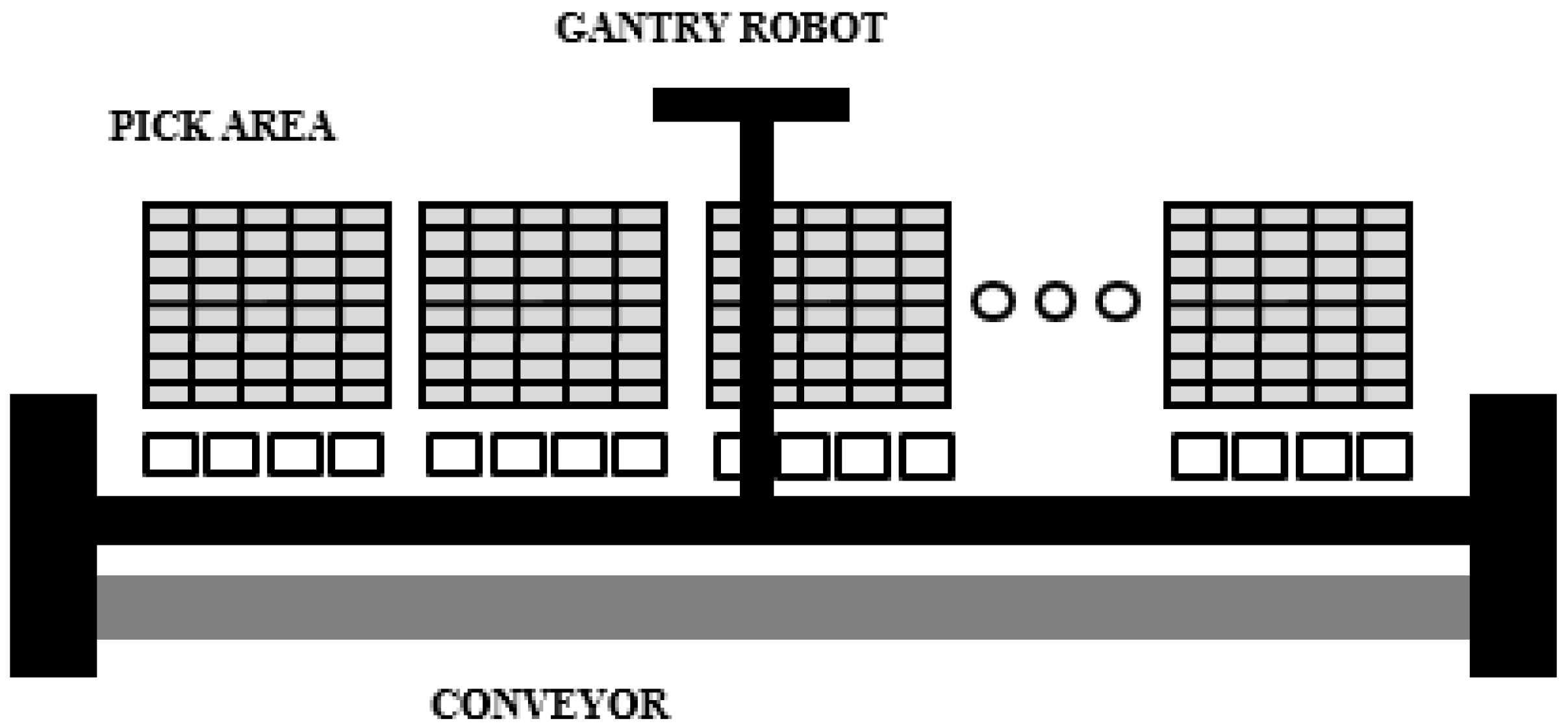
4.1. The Order-Picking Process
4.2. The Order-Picking Scheduling
4.2.1. Order Batching
4.2.2. Order Sequencing
- (1)
- use the X-coordinate based heuristic [63]. The sequencing of orders in each zone is done based on the increasing order of the X-coordinates of the SKU type locations, assuming that the length of each zone is much longer than its width.
- (2)
- Choose randomly the pick locations in each zone.
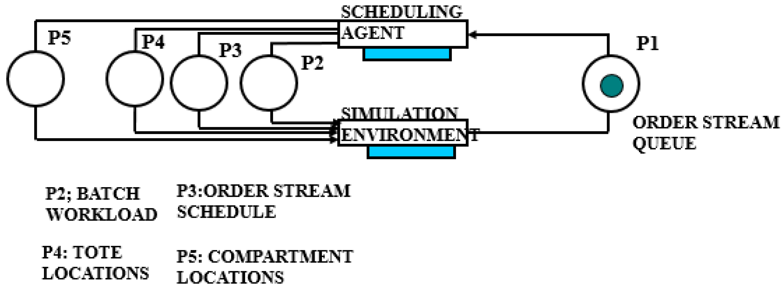
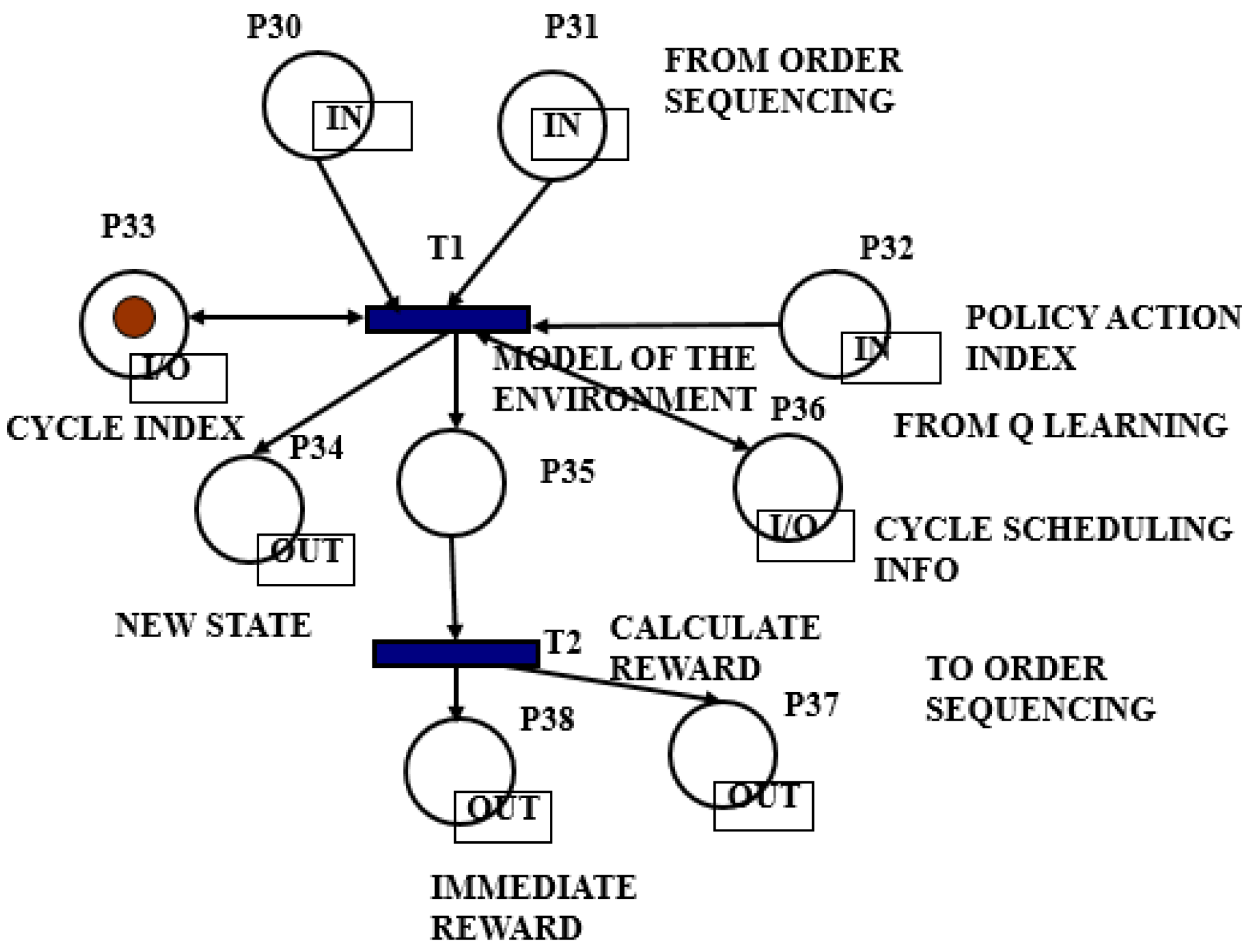
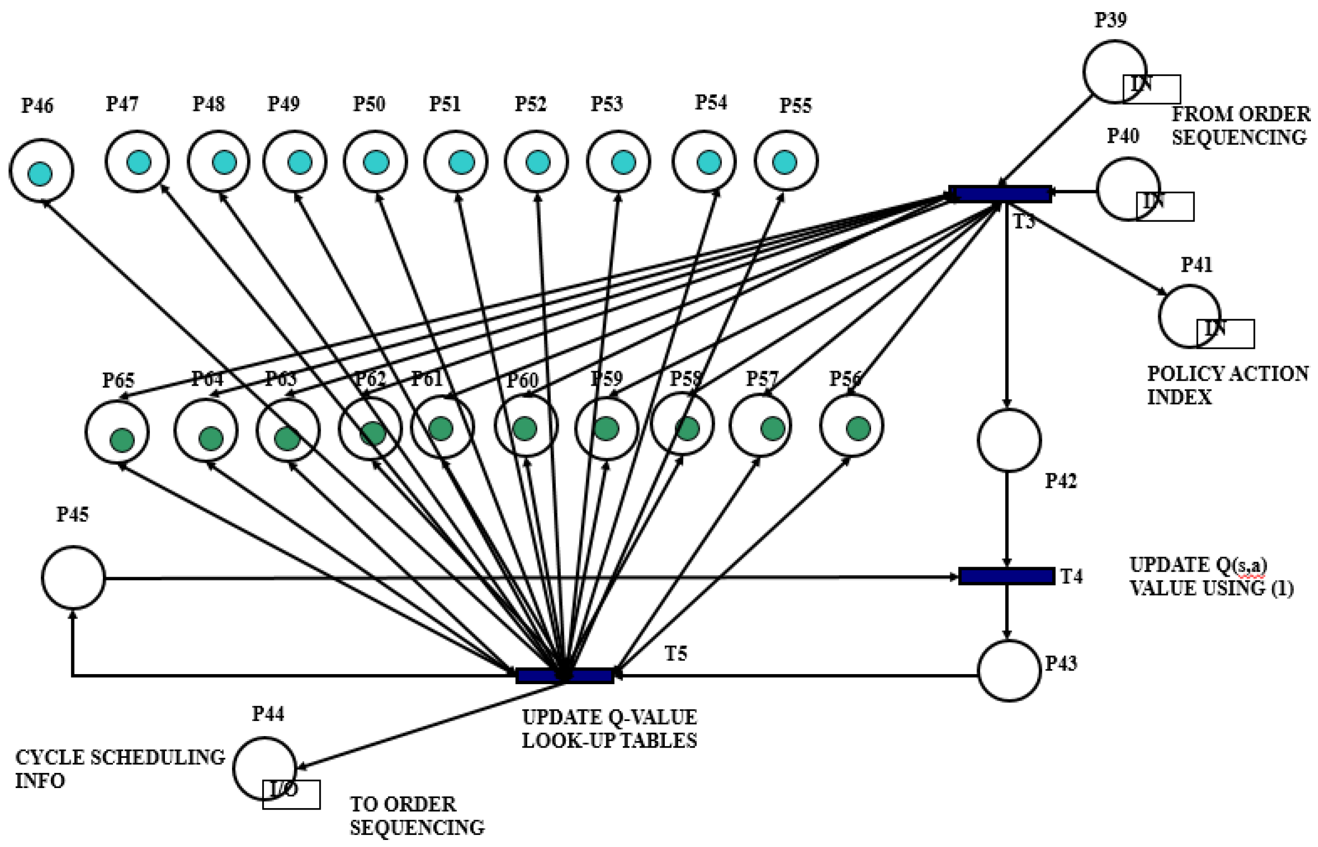
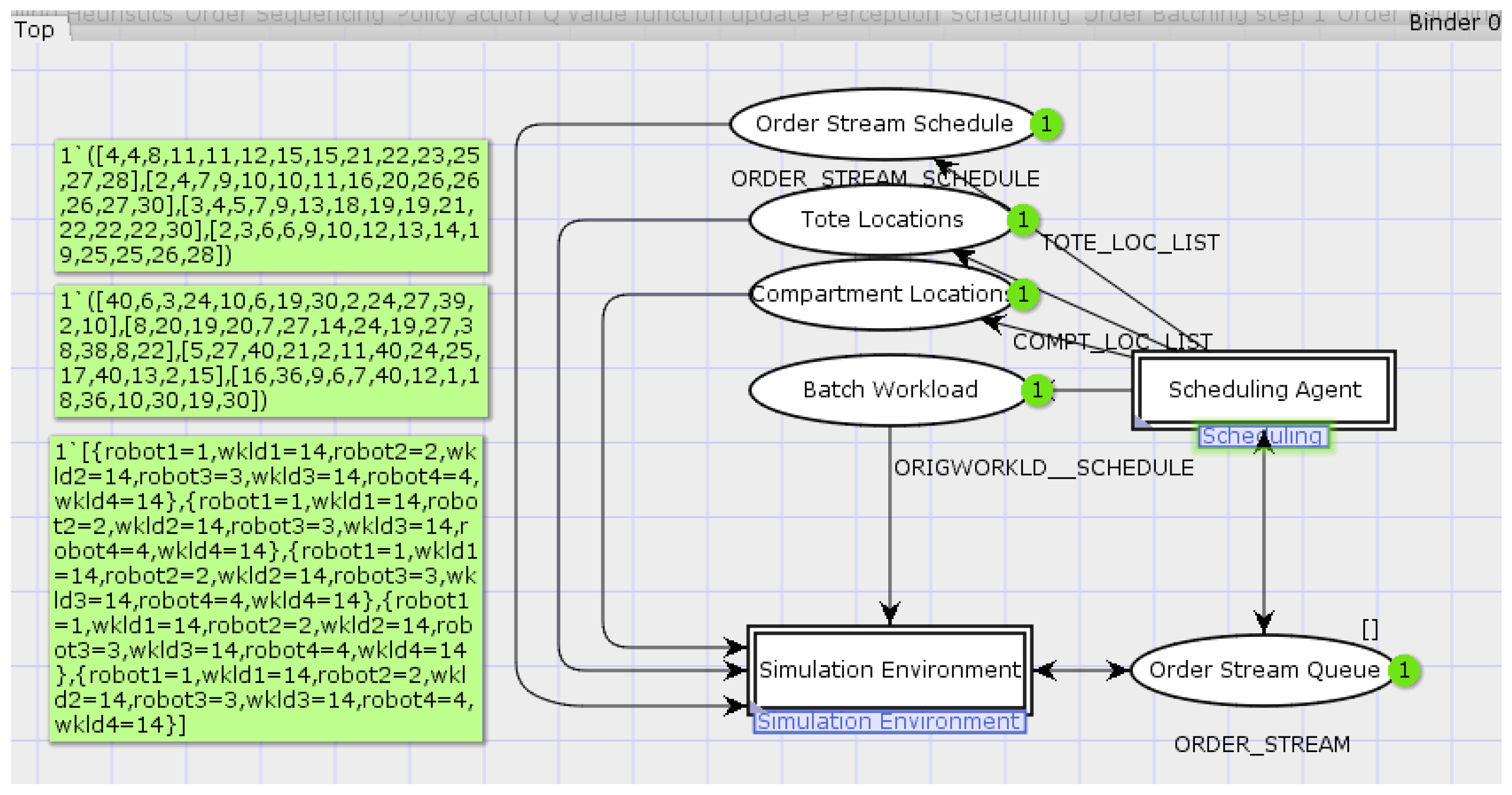
4.3. The Implemented CTPN System Model
5. Simulation and State Space Results
5.1. Validation of the Scheduling Method
5.2. Case Study Performance Evaluation
6. Conclusions
Author Contributions
Conflicts of Interest
References
- Shen, W.; Wang, L.; Hao, Q. Agent-Based Distributed Manufacturing Process Planning and Scheduling: A State-of the-Art Survey. IEEE Trans. Syst. Man Cybern. 2006, 36, 563–577. [Google Scholar] [CrossRef]
- Leitao, P. Agent-based distributed manufacturing control: A state-of-the-art survey. Eng. Appl. Artif. Intell. 2009, 22, 979–991. [Google Scholar] [CrossRef]
- Lee, D.Y.; DiCesare, F. Scheduling flexible manufacturing systems using Petri nets and heuristic search. IEEE Trans. Robot. Autom. 1994, 10, 123–133. [Google Scholar] [CrossRef]
- Shen, W.; Maturana, F.; Norrie, D.H. Enhancing the performance of an agent-based manufacturing system through learning and forecasting. J. Intell. Manuf. 2000, 11, 365–380. [Google Scholar] [CrossRef]
- Wooldridge, M.; Jennings, N.R. Intelligent agents: Theory and practice. Knowl. Eng. Rev. 1995, 10, 115–152. [Google Scholar] [CrossRef]
- Sutton, R.S.; Barto, A.G. Reinforcement Learning: An Introduction; The MIT Press: Cambridge, MA, USA, 1999. [Google Scholar]
- Watkins, C.J.; Dayan, P. Q-learning. Mach. Learn. 1992, 8, 279–292. [Google Scholar] [CrossRef]
- Murata, T. Petri-Nets: Properties, Analysis and Applications. Proc. IEEE. 1989, 77, 541–580. [Google Scholar] [CrossRef]
- Reisig, W. Petri Nets: An Introduction. In EATCS Monographs on Theoretical Computer Science; Springer: Berlin/Heidelberg, Germany, 1985. [Google Scholar]
- Lin, J.T.; Lee, C.C. A Petri net-based integrated control and scheduling scheme for flexible manufacturing cells. Comput. Integr. Manuf. 1997, 10, 109–122. [Google Scholar] [CrossRef]
- Zhou, M.C.; McDermott, K.; Patel, P.A. Petri Net Synthesis and Analysis of a Flexible Manufacturing System Cell. IEEE Trans. Syst. Man. Cybern. 1993, 23, 523–531. [Google Scholar] [CrossRef]
- Wu, N. Necessary and Sufficient Conditions for Deadlock-Free Operation in Flexible Manufacturing Systems Using a Colored Petri Net Model. IEEE Trans. Syst. Man Cybern. C 1999, 29, 129–204. [Google Scholar]
- Tuncel, G.; Bayhan, G.M. Applications of Petri nets in production scheduling: A review. Int. J. Adv. Manuf. Technol. 2007, 34, 762–773. [Google Scholar] [CrossRef]
- Jensen, K.; Kristensen, L.M. Coloured Petri Nets: Modelling and Validation of Concurrent Systems; Springer: Berlin/Heidelberg, Germany, 2009. [Google Scholar]
- Narciso, M.E.; Piera, M.A.; Guasch, A. A time stamp reduction method for state space exploration using colored Petri nets. Simulation 2012, 88, 592–616. [Google Scholar] [CrossRef]
- Piera, M.A.; Narciso, M.; Guasch, A.; Riera, D. Optimization of logistic and manufacturing systems through simulation: A colored Petri net-based methodology. Simulation 2004, 80, 121–130. [Google Scholar] [CrossRef]
- Moore, K.E.; Gupta, S.M. Petri net models of flexible and automated manufacturing systems: A survey. Int. J. Prod. Res. 1996, 34, 3001–3035. [Google Scholar] [CrossRef]
- Hatano, I.; Yamagata, K.; Tamura, H. Modeling and on-line scheduling of flexible manufacturing systems using stochastic Petri nets. IEEE Trans. Softw. Eng. 1991, 17, 126–133. [Google Scholar] [CrossRef]
- Camurri, A.; Franchi, P.; Gandolfo, F.; Zaccaria, R. Petri net based process scheduling: A model of the control system of flexible manufacturing systems. J. Intell. Robot. Syst. 1993, 8, 99–123. [Google Scholar] [CrossRef]
- Chiola, G.; Dutheillet, C.; Franceschinis, G.; Haddad, S. Stochastic well-formed colored nets and symmetric modeling applications. IEEE Trans. Comput. 1993, 42, 1343–1360. [Google Scholar] [CrossRef]
- Castiglione, A.; Gribaudo, M.; Iacono, M.; Palmieri, F. Modeling performances of concurrent big data applications. Softw. Pract. Exp. 2015, 45, 1127–1144. [Google Scholar] [CrossRef]
- Shih, H.; Sekiguchi, T. A timed Petri net and beam search based on-line FMS scheduling system with routing flexibility. In Proceedings of the 1991 IEEE International Conference on Robotics and Automation, Sacramento, CA, USA, 1991; pp. 2548–2553.
- Chen, Q.; Luh, J.Y.S.; Shen, L. Complexity reduction for optimization of deterministic timed Petri-net scheduling by truncation. Cybern. Syst. 1994, 25, 643–695. [Google Scholar] [CrossRef]
- Zhou, M.C.; Xiong, H.H. Petri net scheduling of FMS using branch-and-bound method. In Proceedings of the 1995 IEEE International Conference on Industrial Electronics, Control, and Instrumentation, Orlando, FL, USA, 6–10 November 1995; pp. 211–216.
- Sun, T.H.; Cheng, C.W.; Fu, L.C. Petri net based approach to modeling and scheduling for an FMS and a case study. IEEE Trans. Ind. Electron. 1994, 41, 593–601. [Google Scholar]
- Xiong, H.H.; Zhou, M.C. Scheduling of semiconductor test facility via Petri nets and hybrid heuristic search. IEEE Trans. Semicond. Manuf. 1998, 11, 384–393. [Google Scholar] [CrossRef]
- Jeng, M.D.; Chen, S.C. Heuristic search approach using approximate solutions to Petri net state equations for scheduling flexible manufacturing systems. Int. J. Flex. Manuf. Syst. 1998, 10, 139–162. [Google Scholar] [CrossRef]
- Jeng, M.D.; Lin, C.S.; Huang, Y.S. Petri net dynamics-based scheduling of flexible manufacturing systems with assembly. J. Intell. Manuf. 1999, 10, 541–555. [Google Scholar] [CrossRef]
- Reyes, A.; Yu, H.; Kelleher, G.; Lloyd, S. Integrating Petri Nets and hybrid heuristic search for the scheduling of FMS. Comput. Ind. 2002, 47, 123–138. [Google Scholar] [CrossRef]
- Yu, H.; Reyes, A.; Cang, S.; Lloyd, S. Combined Petri nets modelling and AI-based heuristic hybrid search for flexible manufacturing systems-part II. Heuristic hybrid search. Comput. Ind. Eng. 2003, 44, 545–566. [Google Scholar] [CrossRef]
- Mejía, G.; Odrey, N.G. An approach using Petri Nets and improved heuristic search for manufacturing system scheduling. J. Manuf. Syst. 2005, 24, 79–92. [Google Scholar] [CrossRef]
- Lee, J.; Lee, J.S. Heuristic search for scheduling flexible manufacturing systems using lower bound reachability matrix. Comput. Ind. Eng. 2010, 59, 799–806. [Google Scholar] [CrossRef]
- Huang, B.; Jiang, R.; Zhang, G. Search strategy for scheduling flexible manufacturing systems simultaneously using admissible heuristic functions and nonadmissible heuristic functions. Comput. Ind. Eng. 2014, 71, 21–26. [Google Scholar] [CrossRef]
- Kim, Y.W.; Suzuki, T.; Narikiyo, T. FMS scheduling based on timed Petri Net model and reactive graph search. Appl. Math. Model. 2007, 31, 955–970. [Google Scholar] [CrossRef]
- Mejía, G.; Montoya, C. A Petri net based algorithm for scheduling manufacturing systems with blocking. Int. J. Prod. Res. 2009, 47, 6261–6277. [Google Scholar] [CrossRef]
- Odrey, N.; Mejia, G. An augmented Petri net approach for error recovery in manufacturing systems control. Robot. Comput. Integr. Manuf. 2005, 21, 346–354. [Google Scholar] [CrossRef]
- Murata, T.; Nelson, P.C.; Yim, J. A predicate-transition net model for multiple agent planning. Inf. Sci. 1991, 57, 361–384. [Google Scholar] [CrossRef]
- Leitao, P.; Colombo, A.W.; Restivo, F. An approach to the formal specification of holonic control systems. In Lecture Notes in Computer Science, Holonic and Multi-Agent Systems for Manufacturing, Proceedings of the First International Conference on Industrial Applications of Holonic and Multi-Agent Systems, Prague, Czech Republic, 1–3 September 2003; Springer: Berlin/Heidelberg, Germany, 2003; Volume 2744, pp. 59–70. [Google Scholar]
- Hsieh, F.S. Model and control holonic manufacturing systems based on fusion of contract nets and petri nets. Automatica 2004, 40, 51–57. [Google Scholar] [CrossRef]
- Giglio, D.; Paolucci, M. Agent-based Petri net models for AGV management in manufacturing systems. In Proceedings of the IEEE International Conference on Systems, Man, and Cybernetics, Tucson, AZ, USA, 7–10 October 2001; Volume 4, pp. 2457–2462.
- Castelnuovo, A. Petri net models of agent-based control of a FMS with randomly generated recipes. In Proceedings of the 10th IEEE Conference on Emerging Technologies and Factory Automation, Catania, Italy, 19–22 September 2005; Volume 1, pp. 935–942.
- Bai, Q.; Ren, F.; Zhang, M.; Fulcher, J. CPN-Based State Analysis and Prediction for Multi-agent Scheduling and Planning. In Advances in Agent-Based Complex Automated Negotiations, Studies in Computational Intelligence; Ito, T., Zhang, M., Robu, V., Fatima, S., Matsuo, T., Eds.; Springer: Berlin/Heidelberg, Germany, 2009; Volume 233, pp. 161–176. [Google Scholar]
- Demongodin, I.; Hennet, J.C. A Petri net model of distributed control in a holonic Manufacturing Execution System. In Proceedings of the 17th World Congress, the International Federation of Automatic Control, Seoul, Korea, 6–11 July 2008; pp. 6–11.
- Drakaki, M.; Tzionas, P. Modeling and performance evaluation of an agent-based warehouse dynamic resource allocation using Colored Petri Nets. Int. J. Comput. Integr. Manuf. 2016, 29, 736–753. [Google Scholar] [CrossRef]
- Huang, G.Y. Analysis of Artificial Intelligence Based Petri Net Approach to Intelligent Integration of Design. In Proceedings of the IEEE International Conference on Machine Learning and Cybernetics, Dalian, China, 13–16 August 2006; pp. 1691–1695.
- Chen, S.M.; Ke, J.S.; Chang, J.F. Knowledge representation using fuzzy Petri nets. IEEE Trans. Knowl. Data Eng. 1990, 2, 311–319. [Google Scholar] [CrossRef]
- Joseph, J. Petri nets and the application to artificial intelligence. In Proceedings of the IEEE Colloquium on Software Engineering Practices for Intelligent Knowledge-Based Systems, London, UK, 17 March 1989; pp. 411–414.
- Zha, X.F.; Lim, S.Y.; Fok, S.C. Concurrent intelligent design and assembly planning: Object-oriented intelligent Petri nets approach. In Proceedings of the 1997 IEEE Conference on Systems, Man, and Cybernetics, Orlando, FL, USA, 12–15 October 1997; pp. 30–39.
- Zha, X.F.; Lim, S.Y.E.; Fok, S.C. Integration of knowledge-based systems and neural networks: Neuro-expert Petri net models and applications. In Proceedings of the 1998 IEEE International Conference on Robotics and Automation, Leuven, Belgium, 16–21 May 1998.
- Jávor, A. Petri nets and AI in modeling and simulation. Math. Comput. Simul. 1995, 39, 477–484. [Google Scholar] [CrossRef]
- Aydin, M.E.; Oztemel, E. Dynamic job-shop scheduling using reinforcement learning agents. Robot. Auton. Syst. 2000, 33, 169–178. [Google Scholar] [CrossRef]
- Russell, S.; Norvig, P. Artificial Intelligence: A Modem Approach; Prentice-Hall: Englewood Cliffs, NJ, USA, 1995. [Google Scholar]
- Wang, Y.C.; Usher, J.M. Application of reinforcement learning for agent-based production scheduling. Eng. Appl. Artif. Intell. 2005, 18, 73–82. [Google Scholar] [CrossRef]
- Zhang, W.; Dietterich, T.G. A reinforcement learning approach to job-shop scheduling. In Proceedings of the 14th International Joint Conference on Artificial Intelligence, Montreal, QC, Canada, 20–25 August 1995; pp. 1114–1120.
- Mahadevan, S.; Marchalleck, N.; Das, T.K.; Gosavi, A. Self-improving factory simulation using continuous-time average reward reinforcement learning. In Proceedings of the 14th International Machine Learning Conference, Nashville, TN, USA, 8–12 July 1997; pp. 202–210.
- Das, T.K.; Gosavi, A.; Mahadevan, S.; Marchalleck, N. Solving semi-Markov decision problems using average reward reinforcement learning. Manag. Sci. 1999, 45, 560–574. [Google Scholar] [CrossRef]
- Mahadevan, S.; Theocharous, G. Optimizing production manufacturing using reinforcement learning. In Proceedings of the Eleventh International FLAIRS Conference, Sanibel Island, FL, USA, 18–20 May 1998; pp. 372–377.
- Paternina-Arboleda, C.D.; Das, T.K. Intelligent dynamic control policies for serial production lines. IIE Trans. 2001, 33, 65–77. [Google Scholar] [CrossRef]
- Paternina-Arboleda, C.D.; Das, T.K. A multi-agent reinforcement learning approach to obtaining dynamic control policies for stochastic lot scheduling problem. Simul. Model. Pract. Theory 2005, 13, 389–406. [Google Scholar] [CrossRef]
- Gabel, T.; Riedmiller, M. Adaptive reactive job-shop scheduling with reinforcement learning agents. Int. J. Inf. Technol. Intell. Comput. 2008, 24. [Google Scholar]
- Csáji, B.C.; Monostori, L.; Kádár, B. Reinforcement learning in a distributed market-based production control system. Adv. Eng. Inform. 2006, 20, 279–288. [Google Scholar] [CrossRef]
- Khachatryan, M.; McGinnis, L.F. Picker Travel Time Model for an Order Picking System with Buffers. IIE Trans. 2014, 46, 894–904. [Google Scholar] [CrossRef]
- Kim, B.; Graves, R.J.; Heragu, S.S.; Onge, A.S. Intelligent agent modeling of an industrial warehousing problem. IIE Trans. 2002, 34, 601–612. [Google Scholar] [CrossRef]
- Jensen, K.; Kristensen, L.M.; Wells, L. Coloured Petri Nets and CPN Tools for modelling and validation of concurrent systems. Int. J. Softw. Tools Technol. Trans. 2007, 9, 213–254. [Google Scholar] [CrossRef]
- Fisher, H.; Thompson, G.L. Probabilistic learning combinations of local job-shop scheduling rules. In Industrial Scheduling; Muth, J.F., Thompson, G.L., Eds.; Prentice-Hall: Englewood Cliffs, NJ, USA, 1963; pp. 225–251. [Google Scholar]


| State | State Definition | X-Coordinate Based Heuristic-Q(s,a) Pair | Random Pick Location Selection-Q(s,a) Pair |
|---|---|---|---|
| Dummy | Initial state: total robot travel time (ttot) = 0 | 0 | 0 |
| Dummy | Terminal state:0.98 × ttot,aver ≤ ttot ≤ 1.02 × ttot,aver | 0 | 0 |
| 1 | 0.95 × ttot,aver ≤ ttot ≤ 1.05 × ttot,aver | Q(1,1) | Q(2,1) |
| 2 | 0.9 × ttot,aver ≤ ttot ≤ 1.1 × ttot,aver | Q(2,1) | Q(2,2) |
| 3 | 0.85 × ttot,aver ≤ ttot ≤ 1.15 × ttot,aver | Q(3,1) | Q(3,2) |
| 4 | 0.8 × ttot,aver ≤ ttot ≤ 1.2 × ttot,aver | Q(4,1) | Q(4,2) |
| 5 | 0.75 × ttot,aver ≤ ttot ≤ 1.25 × ttot,aver | Q(5,1) | Q(5,2) |
| 6 | 0.7 × ttot,aver ≤ ttot ≤ 1.3 × ttot,aver | Q(6,1) | Q(6,2) |
| 7 | 0.65 × ttot,aver ≤ ttot ≤ 1.35 × ttot,aver | Q(7,1) | Q(7,2) |
| 8 | 0.6 × ttot,aver ≤ ttot ≤ 1.4 × ttot,aver | Q(8,1) | Q(8,2) |
| 9 | 0.55 × ttot,aver ≤ ttot ≤ 1.45 × ttot,aver | Q(9,1) | Q(9,2) |
| 10 | 0.55 × ttot,aver > ttot, ttot > 1.45 × ttot,aver | Q(10,1) | Q(10,2) |
| If 0.95 × ttot,aver ≤ ttot ≤ 1.05 × ttot,aver then r = 4.5 |
| If 0.9 × ttot,aver ≤ ttot ≤ 1.1 × ttot,aver then r = 4.0 |
| If 0.85 × ttot,aver ≤ ttot ≤ 1.15 × ttot,aver then r = 3.0 |
| If 0.8 × ttot,aver ≤ ttot ≤ 1.2 × ttot,aver then r = 2.5 |
| If 0.75 × ttot,aver ≤ ttot ≤ 1.25 × ttot,aver then r = 2.0 |
| If 0.7 × ttot,aver ≤ ttot ≤ 1.3 × ttot,aver then r = 1.0 |
| If 0.65 × ttot,aver ≤ ttot ≤ 1.35 × ttot,aver then r = −1.0 |
| If 0.6 × ttot,aver ≤ ttot ≤ 1.4 × ttot,aver then r = −2.0 |
| If 0.55 × ttot,aver ≤ ttot ≤ 1.45 × ttot,aver then r = −3.0 |
| If 0.55 × ttot,aver > ttot, ttot > 1.45 × ttot,aver then r = −4.0 |
| colset INTT = INT timed; colset REALT = real timed; colset Order = record orderno:INT*prodno:INT*itemno:INT*AT:INT; colset ORDER_STREAM = list Order timed; colset ORDER_SCHEDULE = list ORDER_STREAM; colset ORIGWORKLDn = record robot1:INT*wkld1:INT*robot2:INT*wkld2:INT* robot3:INT*wkld3:INT*robot4:INT*wkld4:INT; colset ORIGWORKLD_SCHEDULE = list ORIGWORKLDn; colset BATCH_INFO = record batch_ord:INT*batch_wkld: ORDER_STREAM* batch_itm_cnt:INT; colset BATCH_LIST = list BATCH_INFO; colset ORDERinBATCH = record orderid:INT*prodno:INT*lnitmno:INT*pickzono:INT; colset BATCH_of_ORDERS = list ORDERinBATCH; colset ORDER_STREAM_SCHEDULE = list BATCH_of_ORDERS; colset PZ1_LOC_LIST = list INT timed; colset TOTE_LOC_LIST = PZ1_LOC_LISTxPZ2_LOC_LISTxPZ3_LOC_LISTxPZ4_LOC_LIST; colset COMPT_LOC_LIST = PZ1_LOC_LISTxPZ2_LOC_LISTxPZ3_LOC_LISTxPZ4_LOC_LIST; colset QVAL = list REAL timed; colset CYCLE_SCHEDULE_INFO = list REALxINTxREALxREALxREALxREAL; |
| Benchmark Example | Optimal Makespan | Xiong and Zhou [26] | Huang et al. [33] | Yu et al. [30] | Gabel and Riedmiller [60] | This Study |
|---|---|---|---|---|---|---|
| Xiong and Zhou (1998)-lot size (1,1,1,1) [26] | 17 | 17 | 17 | 17 | - | 17 (50%) |
| Xiong and Zhou (1998)-lot size (5,5,2,2) [26] | 58 | 58 | 58 | 58 | - | 58 (52%) |
| Xiong and Zhou (1998)-lot size (10,10,6,6) [26] | 134 | 134 | 134 | 134 | - | 134 (42%) |
| Fisher and Thompson (1963)-ft6 6x6 [65] | 55 | - | - | - | 57 | 57 (0.1%) |
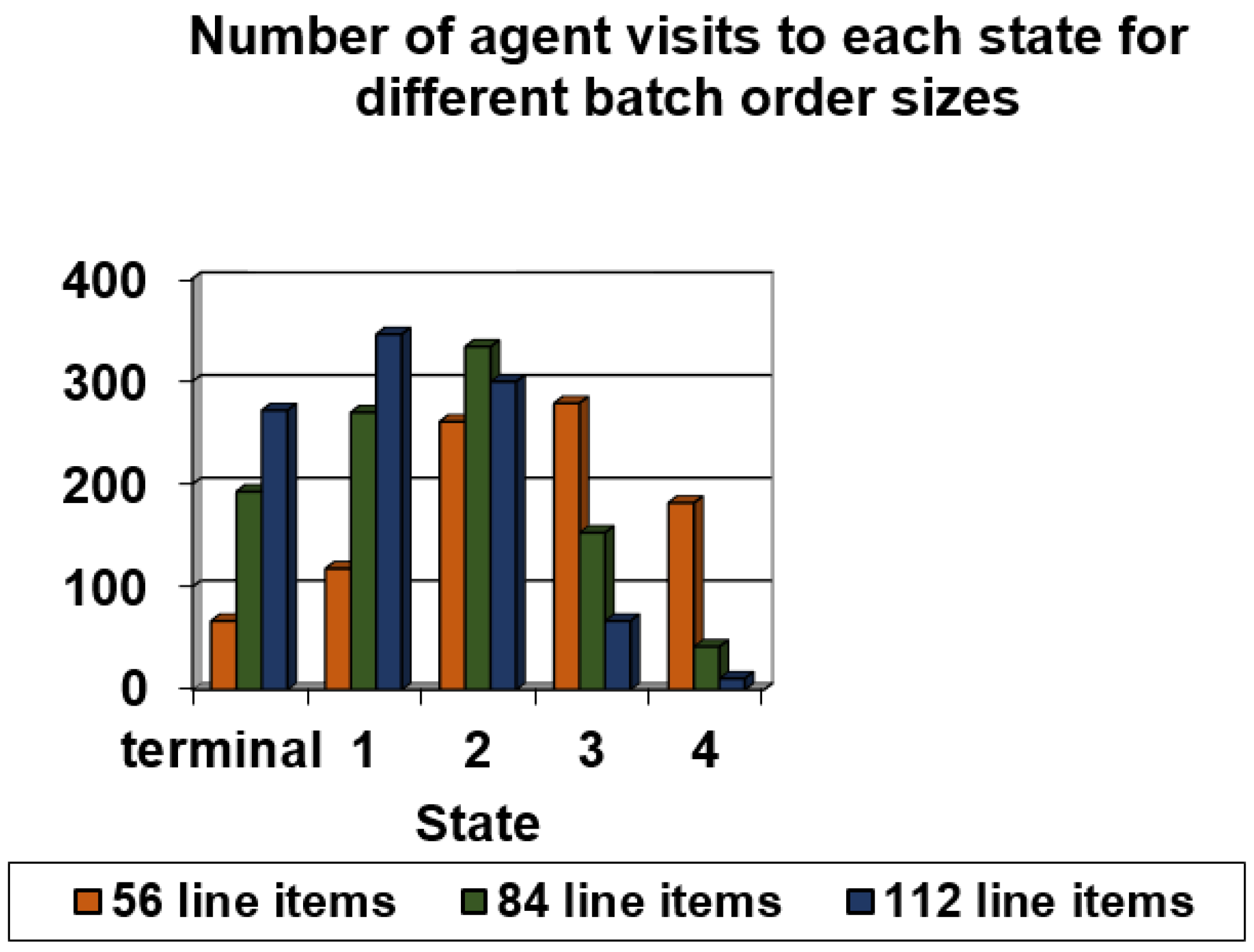
| Total Number of Line Items in Batch | Policy Action | Number of Visits to Terminal State | Number of Visits to State 1 | Number of Visits to State 2 | Number of Visits to State 3 | Number of Visits to State 4 | Total Robot Travel Time, ttot, (ttot,aver) |
|---|---|---|---|---|---|---|---|
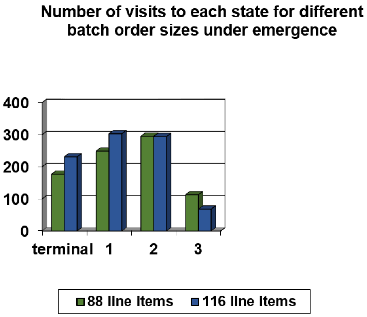
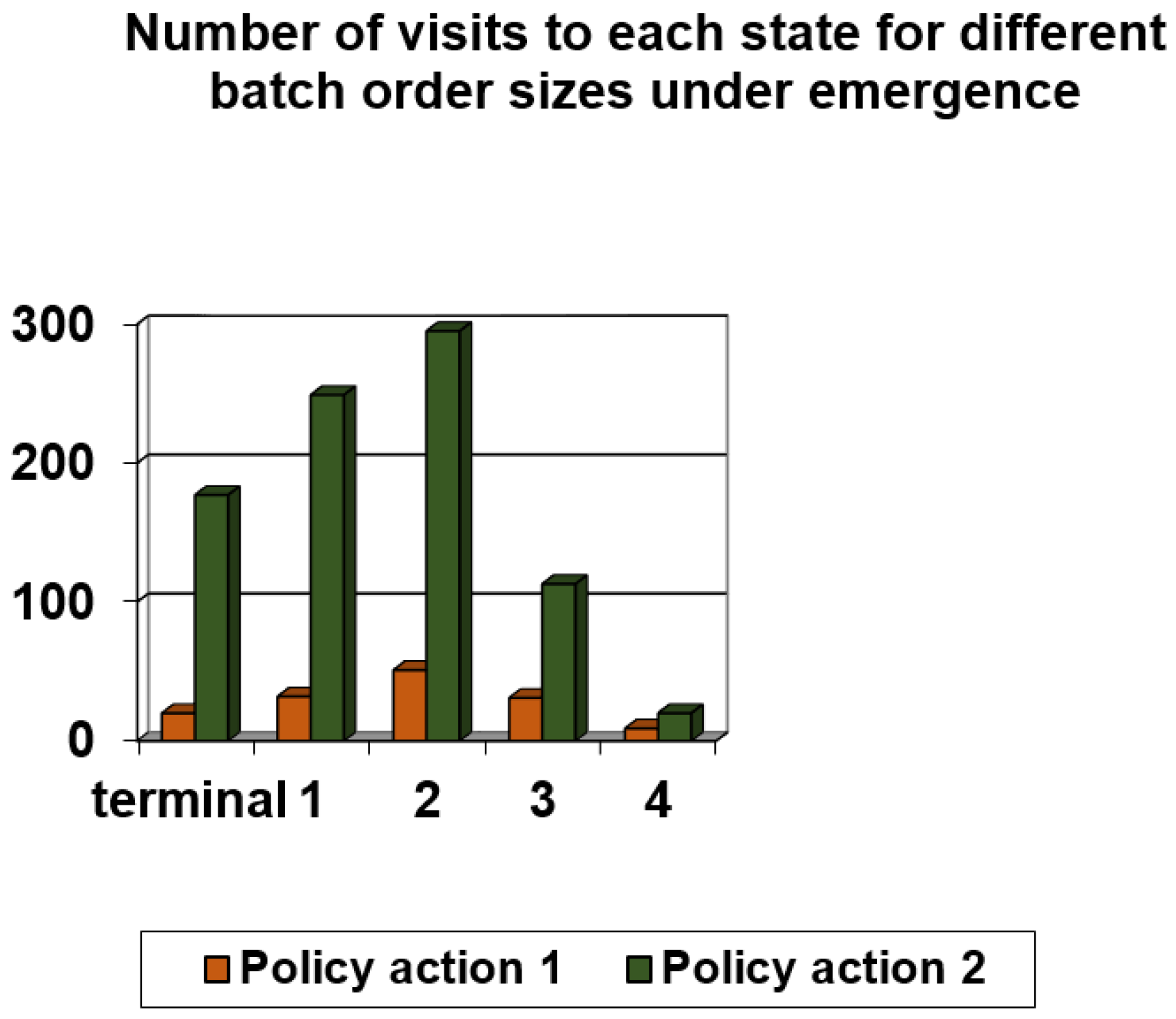
| 56 line items | 1 | 67 | 118 | 261 | 279 | 182 | 341.84 (340.92) |
| 84 line items | 1 | 193 | 270 | 334 | 153 | 42 | 514.14 (513.68) |
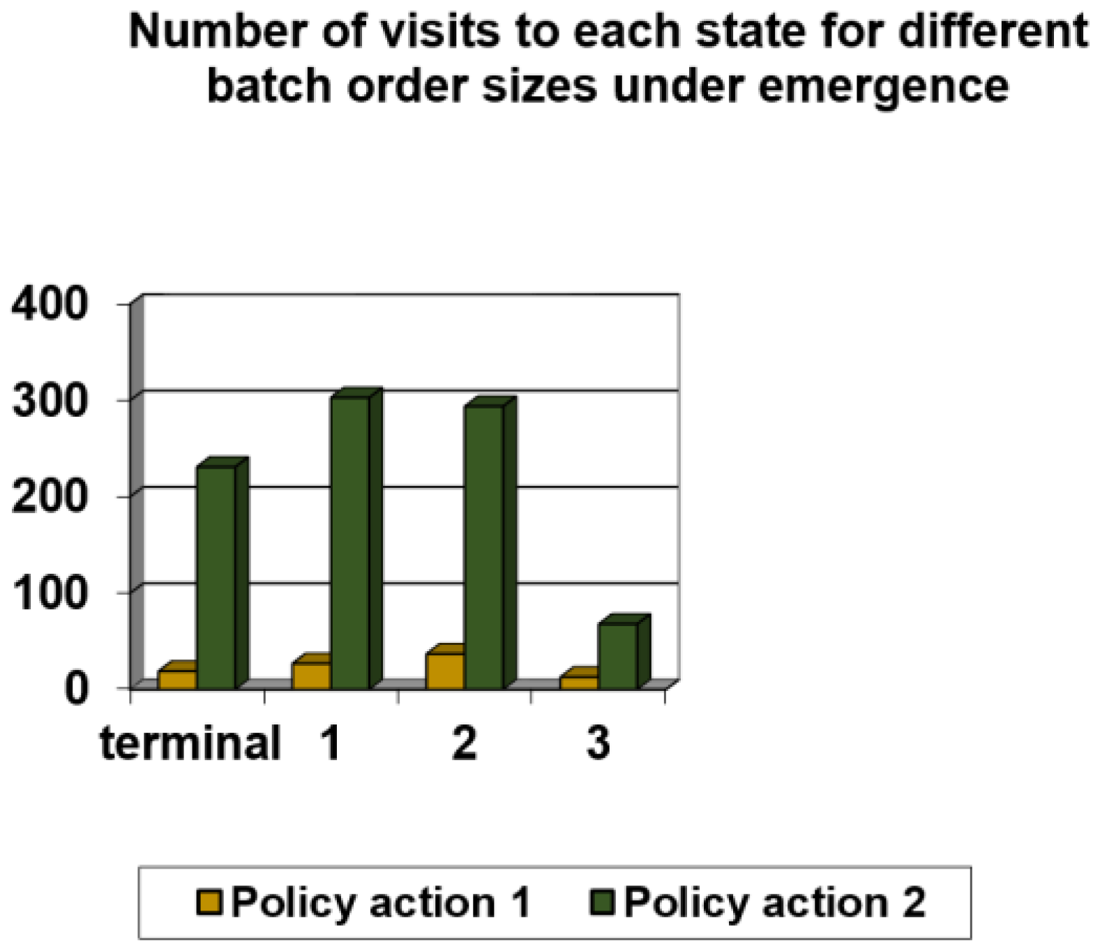
| 112 line items | 1 | 272 | 346 | 300 | 67 | 11 | 685.18 (684.72) |
| State | State Definition | 4 Late Orders Assigned to Robot 1 —Q(s,a) Pair | 2 Late Orders Assigned to Robot 1 and 2 Late Orders to Robot 2 —Q(s,a) Pair |
|---|---|---|---|
| Dummy | Initial state: total robot travel time (ttot) = 0 | 0 | 0 |
| Dummy | Terminal state: 0.85 × ttot,aver ≤ ttot,robot1 ˄ ttot,robot2 ˄ ttot,robot3 ˄ ttot,robot4 ≤ 1.15 × ttot,aver | 0 | 0 |
| 1 | 0.8 × ttot,aver ≤ ttot,robot1 ˄ ttot,robot2 ˄ ttot,robot3 ˄ ttot,robot4 ≤ 1.2 × ttot,aver | Q(1,1) | Q(2,1) |
| 2 | 0.75 × ttot,aver ≤ ttot,robot1 ˄ ttot,robot2 ˄ ttot,robot3 ˄ ttot,robot4 ≤ 1.25 × ttot,aver | Q(2,1) | Q(2,2) |
| 3 | 0.7 × ttot,aver ≤ ttot,robot1 ˄ ttot,robot2 ˄ ttot,robot3 ˄ ttot,robot4 ≤ 1.3 × ttot,aver | Q(3,1) | Q(3,2) |
| 4 | 0.65 × ttot,aver ≤ ttot,robot1 ˄ ttot,robot2 ˄ ttot,robot3 ˄ ttot,robot4 ≤ 1.35 × ttot,aver | Q(4,1) | Q(4,2) |
| 5 | 0.6 × ttot,aver ≤ ttot,robot1 ˄ ttot,robot2 ˄ ttot,robot3 ˄ ttot,robot4 ≤ 1.4 × ttot,aver | Q(5,1) | Q(5,2) |
| 6 | 0.55 × ttot,aver ≤ ttot,robot1 ˄ ttot,robot2 ˄ ttot,robot3 ˄ ttot,robot4 ≤ 1.45 × ttot,aver | Q(6,1) | Q(6,2) |
| 7 | 0.5 × ttot,aver ≤ ttot,robot1 ˄ ttot,robot2 ˄ ttot,robot3 ˄ ttot,robot4 ≤ 1.5 × ttot,aver | Q(7,1) | Q(7,2) |
| 8 | 0.45 × ttot,aver ≤ ttot,robot1 ˄ ttot,robot2 ˄ ttot,robot3 ˄ ttot,robot4 ≤ 1.55 × ttot,aver | Q(8,1) | Q(8,2) |
| 9 | 0.4 × ttot,aver ≤ ttot,robot1 ˄ ttot,robot2 ˄ ttot,robot3 ˄ ttot,robot4 ≤ 1.6 × ttot,aver | Q(9,1) | Q(9,2) |
| 10 | 0.4 × ttot,aver > ttot,robot1 ˄ ttot,robot2 ˄ ttot,robot3 ˄ ttot,robot4, ttot,robot1 ˄ ttot,robot2 ˄ ttot,robot3 ˄ ttot,robot4 > 1.6 × ttot,aver | Q(10,1) | Q(10,2) |
| If 0.85 × ttot,aver ≤ ttot,robot1 ˄ ttot,robot2 ˄ ttot,robot3 ˄ttot,robot4 ≤ 1.15 × ttot,aver then r = 4.5 |
| If 0.8 × ttot,aver ≤ ttot,robot1 ˄ ttot,robot2 ˄ ttot,robot3 ˄ ttot,robot4 t ≤ 1.2 × ttot,aver then r = 4.0 |
| If 0.75 × ttot,aver ≤ ttot,robot1 ˄ ttot,robot2 ˄ ttot,robot3 ˄ ttot,robot4 ≤ 1.25 × ttot,aver then r = 3.0 |
| If 0.7 × ttot,aver ≤ ttot,robot1 ˄ ttot,robot2 ˄ ttot,robot3 ˄ ttot,robot4 ≤ 1.3 × ttot,aver then r = 2.5 |
| If 0.65 × ttot,aver ≤ ttot,robot1 ˄ ttot,robot2 ˄ ttot,robot3 ˄ ttot,robot4 ≤ 1.35 × ttot,aver then r = 2.0 |
| If 0.6 × ttot,aver ≤ ttot,robot1 ˄ ttot,robot2 ˄ ttot,robot3 ˄ ttot,robot4 ≤ 1.4 × ttot,aver then r = 1.0 |
| If 0.55 × ttot,aver ≤ ttot,robot1 ˄ ttot,robot2 ˄ ttot,robot3 ˄ ttot,robot4 ≤ 1.45 × ttot,aver then r = −1.0 |
| If 0.5 × ttot,aver ≤ ttot,robot1 ˄ ttot,robot2 ˄ ttot,robot3 ˄ ttot,robot4 ≤ 1.5 × ttot,aver then r = −2.0 |
| If 0.45 × ttot,aver ≤ ttot,robot1 ˄ ttot,robot2 ˄ ttot,robot3 ˄ ttot,robot4 ≤ 1.55 × ttot,aver then r = −3.0 |
| If 0.45 × ttot,aver > ttot,robot1 ˄ ttot,robot2 ˄ ttot,robot3 ˄ ttot,robot4, ttot,robot1 ˄ ttot,robot2 ˄ ttot,robot3 ˄ ttot,robot4 > 1.55 × ttot,aver then r = −4.0 |
| Scheduling Rule | Pick Zone 1 | Pick Zone 2 | Pick Zone 3 | Pick Zone 4 | Number of Orders per Pick Zone under Normal Conditions |
|---|---|---|---|---|---|
| Policy action 1 | 25 | 21 | 21 | 21 | 21 |
| Policy action 2 | 23 | 23 | 21 | 21 | 21 |
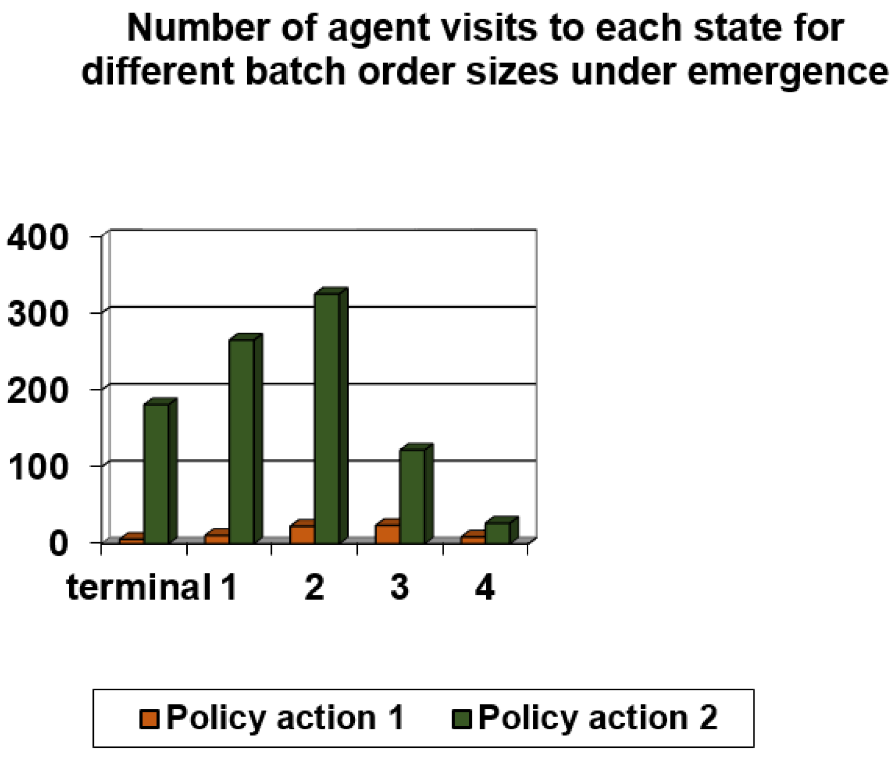
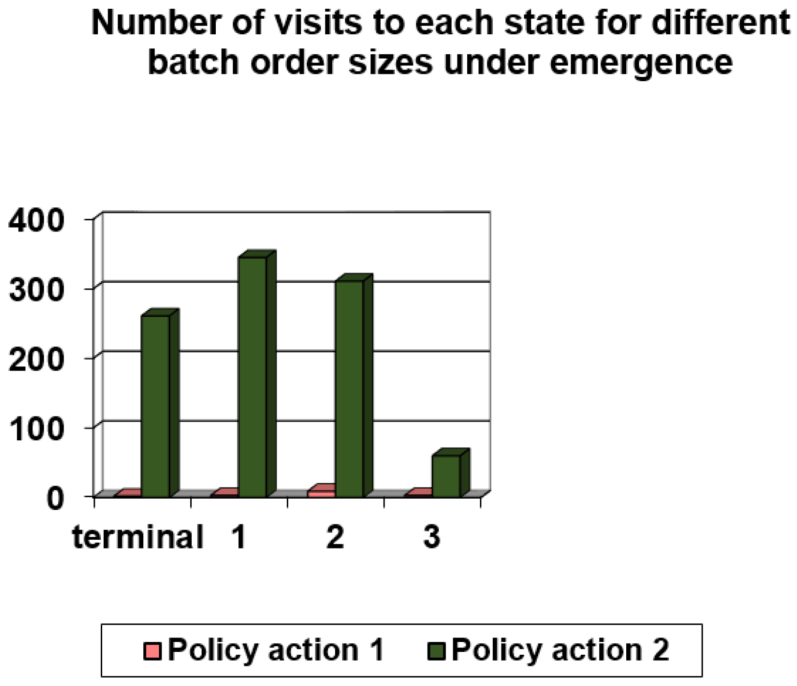
| Scheduling Rule | Number of Visits to Terminal State | Number of Visits to State 1 | Number of Visits to State 2 | Number of Visits to State 3 | Number of Visits to State 4 | Number of Visits to State 5 |
|---|---|---|---|---|---|---|
| Policy action 1 | 6 | 11 | 23 | 24 | 9 | 1 |
| Policy action 2 | 181 | 265 | 325 | 122 | 27 | 4 |
© 2017 by the authors. Licensee MDPI, Basel, Switzerland. This article is an open access article distributed under the terms and conditions of the Creative Commons Attribution (CC BY) license ( http://creativecommons.org/licenses/by/4.0/).
Share and Cite
Drakaki, M.; Tzionas, P. Manufacturing Scheduling Using Colored Petri Nets and Reinforcement Learning. Appl. Sci. 2017, 7, 136. https://doi.org/10.3390/app7020136
Drakaki M, Tzionas P. Manufacturing Scheduling Using Colored Petri Nets and Reinforcement Learning. Applied Sciences. 2017; 7(2):136. https://doi.org/10.3390/app7020136
Chicago/Turabian StyleDrakaki, Maria, and Panagiotis Tzionas. 2017. "Manufacturing Scheduling Using Colored Petri Nets and Reinforcement Learning" Applied Sciences 7, no. 2: 136. https://doi.org/10.3390/app7020136