Beam Grouping Based RS Resource Reuse and De-Contamination in Large Scale MIMO Systems

Abstract

It is well known that large scale multiple-input multiple-output (LS-MIMO) systems are very attractive technology to increase both spectral efficiency (SE) and energy efficiency (EE). However, one of big obstacles to the realization of the LS-MIMO system is the overhead of reference signals (RSs), since the number of RS increases as the number of transmitter (TX) antennas increases. In this paper, the RS overhead problem is analyzed, and we propose an RS overhead reduction scheme based on beam grouping, which is called beam grouping based resource reuse (BGRR). The proposed scheme divides one cell into several sectors and reuses the RS resources for the different sectors. The resource conflict is reduced using beam separability. According to the analysis and the simulation results, the proposed scheme can remarkably reduce the RS overhead and improve the SE performance significantly.

1. Introduction

Large Scale Multiple-Input Multiple-Output (LS-MIMO) systems have received great attention due to the possibility of increasing both spectral efficiency (SE) and energy efficiency (EE). They are already considered to be incorporated into the 3rd generation partnership project (3GPP) standard body, and are referred to as Full-Dimension MIMO (FD-MIMO) systems [1,2,3,4,5]. However, most of the performance analysis for LS-MIMO systems disregard its high implementation complexity and the overhead required for reference signals (RSs). The RS proportionately increases as the number of transmitter (TX) antennas and/or user equipment (UEs) increases. Therefore, solving this problem is required to achieve the expected performance gain introduced in the literature.

The RS overhead reduction is a traditional problem in wireless communication systems. Blind channel estimation technologies using the specific statistical property of the signal and the channel, and the correlation based channel recovery were introduced in [6,7]. This kind of technology can have a very high impact, but it usually requires long observation time and high complexity. Training based super imposed RS on data signals, which locates RS stream and data stream in the same resources, were also introduced in [8,9]. This can give very efficient results for reducing RS overhead because data can be transmitted in all time and frequency resources. However, the performance loss due to data and RS imposition is inevitable.

Generally, the reduction of the RS overhead is considered just for SE, but it becomes a problem for realizing the products in LS-MIMO systems. That is, LS-MIMO would never be realized without the reduction of the RS overhead. For example, if the number of TX antennas is increased up to several dozen, the required RS resource would be more than the available physical resource. Even 3GPP LTE-A Release 10 uses only up to eight antennas, but the RS overhead is more than $30\%$.

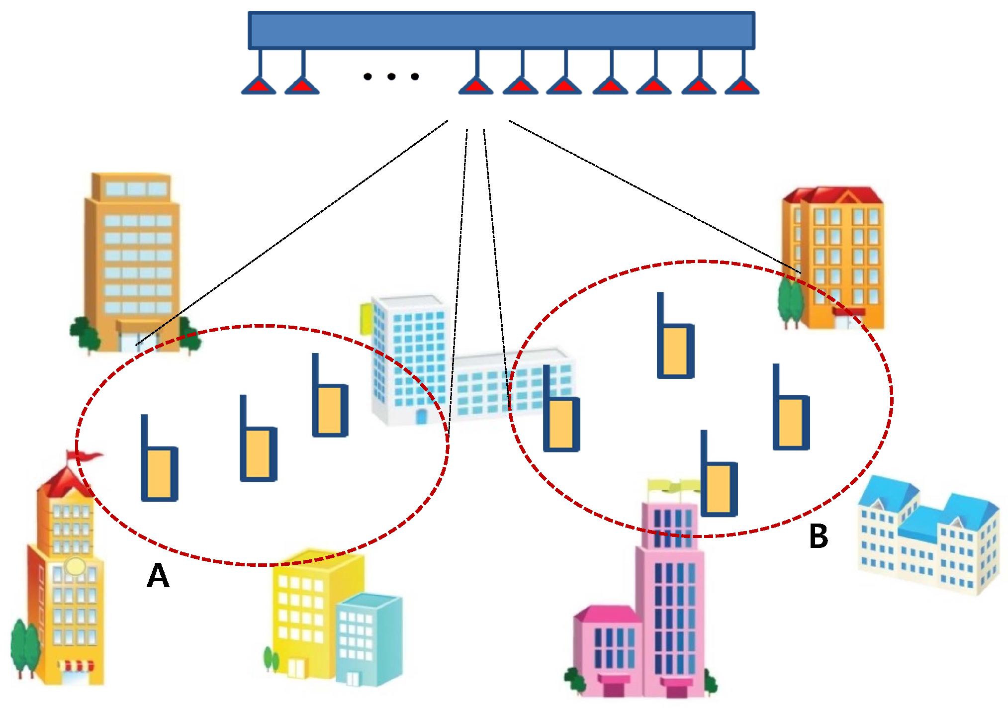
In this paper, the RS overhead problem is analyzed. We then propose an RS overhead reduction scheme, called beam grouping resource reuse (BGRR), and evaluate its performance for various scenarios. The main idea of BGRR scheme is that it makes dynamic virtual sectors by using a beam group in a given cell and reuse the RS resources for different virtual sectors. The high level concept of proposed methodology is given in Figure 1.

For example, we can divide a cell into two different zones using beamforming based on a large scale antenna system, i.e., zone ‘A’ and zone ‘B’ , and regard the two different zones as different sectors (Figure 1). The RS resources used for zone ‘A’ also can be used for zone ‘B’. Then, RS overhead can be reduced by a half compared to without BGRR. Reducing the inter-virtual-sector interference (IVSI) is essential. How to divide the given cell is also a question.

In what follows, the system model for the numerical analysis is shown in Section 2. In Section 3, we present the analysis of the RS overhead. In Section 4, we propose a BGRR scheme, and provide relevant analysis. In Section 5, we present numerical results of the proposed scheme. Section 6 is the concluding remarks.

Notation: In the following, boldface lower-case and upper-case characters denote vectors and matrices, respectively. The operators ${(·)}^H$ and $E[·]$ denote conjugate transpose and expectation, respectively. The $N\times N$ identity matrix is denoted ${\mathbf{I}}_N$, $log(·)$ is the common logarithm and $\mathbf{X}\sim CN(0,{\mathbf{V}}_N)$ is the complex Gaussian distributed vector with mean zero and covariance ${\mathbf{V}}_N$.

2. System Model

This section describes the LS-MIMO model and the channel model. These are necessary to introduce and analyze the proposed scheme.

2.1. LS-MIMO Model

When a downlink LS-MIMO system with $N_t$ TX antennas, and K single antenna receivers (RXs) is considered, the received signal vector at RXs can be represented as follows:

$$\begin{array}{ccc}\hfill \mathbf{y}& =& \sqrt{{\rho }_t}\mathbf{H}\mathbf{s}+\mathbf{z},\hfill \end{array}$$

(1)

where $\mathbf{y}$ is the $K\times 1$ received vector for K UEs, ${\rho }_t$ is the total TX power for forward link, $\mathbf{H}$ is the $K\times N_t$ channel matrix between the transmitter with $N_t$ TX antennas and K RX terminals, $\mathbf{s}$ is the $N_t\times 1$ TX signal vector, and $\mathbf{z}$ is the $K\times 1$ noise (AWGN) vector at the UEs. We only consider the narrowband signal since orthogonal frequency division multiplexing (OFDM) can successfully change the wideband signal to the narrowband signal. We assume the transmitter has perfect channel state information (CSI). Note that usually the LS-MIMO system satisfies the condition of $N_t>10K$.

2.2. Channel Model

A given with the LS-MIMO model, it can be easily expected that there would be some correlation at the TX side but little correlation at the RX side, since the TX side has a large number of TX antennas in a limited space, while the RX side has one antenna in each. The channel can be modeled as follows [10,11]:

$$\begin{array}{}\mathrm{(2)}& \mathbf{H}& \begin{array}{cc}=& {[{\mathbf{g}}_1^T,\cdots ,{\mathbf{g}}_k^T,\cdots ,{\mathbf{g}}_K^T]}^T\circ {[{\mathbf{A}}_1^T,\cdots ,{\mathbf{A}}_k^T,\cdots ,{\mathbf{A}}_K^T]}^T,\hfill \end{array}\mathrm{(3)}& & \begin{array}{cc}=& {[{\mathbf{h}}_1^T,\cdots ,{\mathbf{h}}_k^T,\cdots ,{\mathbf{h}}_K^T,]}^T,\hfill \end{array}\end{array}$$

where ${\mathbf{g}}_k$ is the $1\times D_k$ complex Gaussian vector with mean zero and unit variance (${\mathbf{g}}_k\sim CN(0,{\mathbf{I}}_{D_k})$), $D_k$ is the the number of resolvable directional path from a transmitter antenna to a RX antenna, ${\mathbf{A}}_k\in {\mathbb{C}}^{D_k\times N_t}$ is the transmit steering matrix containing $D_k$ steering vectors of the transmit antenna array, and ∘ is the Hadamard product operation. Then, $1\times N_t$ channel vector for k-th single antenna user can be expressed as

$${\mathbf{h}}_k^{}={\mathbf{g}}_k{\mathbf{A}}_k.$$

(4)

We simply disregard the mutual coupling since it is beyond the scope of this paper. Assuming a uniform linear array at the TX, the steering matrix for the $k^{th}$ UE can be expressed as follows:

$${\mathbf{A}}_k=\frac{1}{\sqrt{D_k}}{\left[{\mathbf{a}}^T\left({\theta }_{k,1}\right),\cdots ,{\mathbf{a}}^T\left({\theta }_{k,D_k}\right)\right]}^T,$$

(5)

where ${\mathbf{a}}^T\left({\theta }_{k,i}\right)$ is given as

$${\mathbf{a}}^{}\left({\theta }_{k,i}\right)=\left[1,e^{j2\pi dsin{\theta }_{k,i}},\cdots ,e^{j2\pi (N_t-1)dsin{\theta }_{k,i}}\right],$$

(6)

where d is the normalized antenna spacing by wavelength. By adjusting the angular spread and the antenna spacing, we can make various channel conditions. In this paper, we assume little angular spread and $0.5\lambda$ antenna spacing.

3. Analysis of RS Overhead

The current 3GPP LTE system, which is considered as a reference model, uses five kinds of RS, i.e., common reference signal (CRS), channel state information reference signal (CSI-RS), demodulation reference signal (DM-RS), multicast-broadcast single-frequency network (MBSFN) reference signal, positioning reference signal (PRS). In this paper, we only consider CRS, CSI-RS, and DM-RS because these three signals take most of the resources for RS. The CRS is usually called a cell specific reference signal and has been in the LTE system from release 8. The role of CRS is cell search and initial acquisition, downlink channel estimation for coherent demodulation/detection at the UE, and downlink channel quality measurements. The CSI-RS has been introduced from release 10 and used by the UE to estimate the channel and report channel quality information (CQI) to the BS. The DM-RS is usually called a UE specific reference signal, and its role is for the demodulation of the signal. The analysis in this paper is from the BS point of view, since the proposed scheme is for LS-MIMO systems, which can be installed in the BS.

Although it is difficult to estimate how technology will be evolved especially for the BS point of view, it is quite obvious that the overhead of RS will be increased as the number of TX antennas is increased. In this section, we present analysis of RS overhead based on several assumptions. In current 3GPP LTE-A systems, the available number of resource elements is 168 (12 (frequency tones) × 14 (time symbols)) and there are 24 CRSs in two resource blocks (1 ms). This means that CRS itself takes $14.8\%$ of available resource elements, which is not a small portion. In this paper, we use the following model for the analysis of RS overhead:

$$\begin{array}{ccc}\hfill {\chi }_{WCR}(\%)& =& ({\eta }_{CRS}+K+K·{\chi }_{DM-RS})/{\eta }_{R{B}_{tot}}\times 100,\hfill \end{array}$$

(7)

$$\begin{array}{ccc}\hfill {\chi }_{WOCR}(\%)& =& ({\eta }_{CRS}+N_t+K·{\chi }_{DM-RS})/{\eta }_{R{B}_{tot}}\times 100,\hfill \end{array}$$

(8)

where ${\chi }_{WCR}(\%)$ and ${\chi }_{WOCR}(\%)$ are the overhead of RS, which are represented in percentage for “with channel reciprocity (WCR)” and “without channel reciprocity (WOCR)” in a given resource, respectively. The WCR means that BS estimates the channel for downlink precoding by using an uplink signal from UE. That is to say, BS measures the channel by using an uplink signal. It indicates that the number of CSI-RS is proportional to the number of UEs, K. This kind of mechanism usually can be used for a TDD system. Uplink/downlink channel calibration is necessary to use an uplink signal for downlink precoding. The WOCR means that BS estimates the channel for precoding by using a feedback signal from UE. That is to say, UE measures the channel by using the downlink RS. It indicates that the number of CSI-RS is proportional to the number of TX antennas, $N_t$. This kind of mechanism can be applicable for both TDD and FDD systems. ${\eta }_{CRS}$ is the number of CRS, and ${\chi }_{DM-RS}$ is the DM-RS proportional factor of K in a given resource ${\eta }_{R{B}_{tot}}$. The second term K in Label (7) and $N_t$ in Label (8) indicate the number of CSI-RS in a given resource ${\eta }_{R{B}_{tot}}$. We assume channel measurement is performed by using CRS and CSI-RS, while demodulation is performed by using DM-RS.

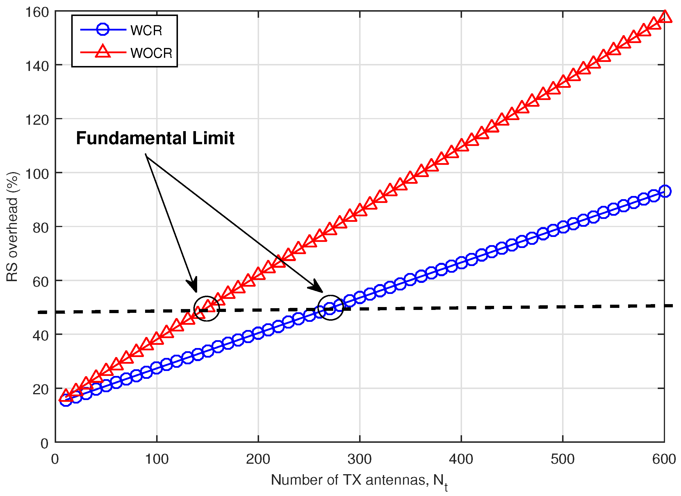
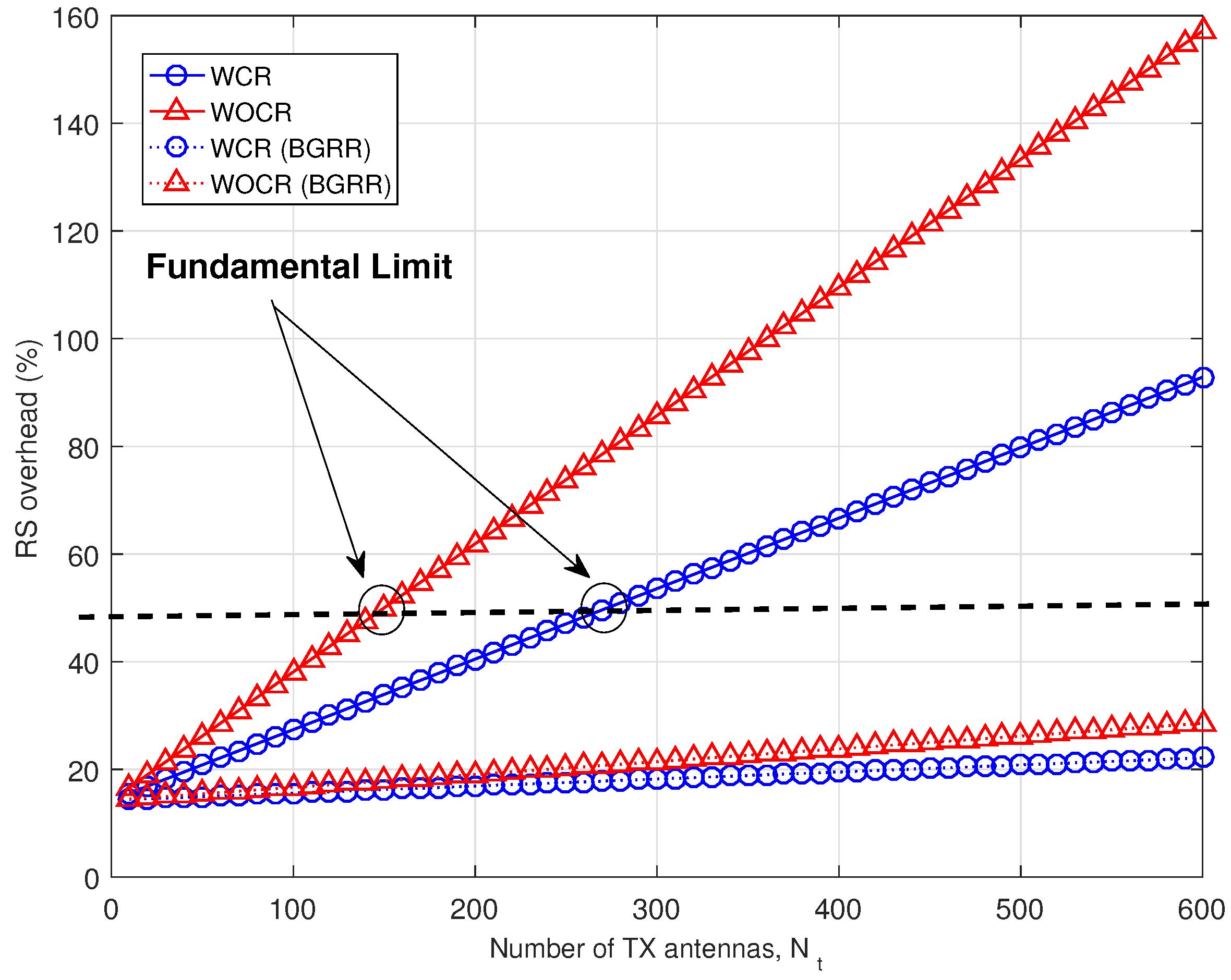
Figure 2 shows the RS overhead (%) versus the number of TX antennas, $N_t$, for 5 ms coherence time, which means nomadic or static channel. Here, we assume K also is increased as $N_t$ is increased, while maintaining $K=0.1N_t$. If we increase the number of TX antennas $N_t$, there is an opportunity to increase the co-scheduled number of UEs, K, with minimum channel hardening effect of LS-MIMO, $N_t=10K$. We also assume that the fundamental limit of overhead of RS is $50\%$, which is corresponding to $N_t=273$ in the case of WCR, and $N_t=150$ in the case of WOCR. If $N_t$ is more than $273/150$, the RS takes more than the data signal, and it is not acceptable from the system performance point of view.

Table 1. Maximum number of allowable transmitter (TX) antennas in a given overhead of reference signal (RS), $\chi (\%)$.

$\mathit{\chi }(\%)$	$25\%$	$50\%$	$65\%$	$80\%$
$N_t\left(WCR\right)$	82	273	387	502
$N_t\left(WOCR\right)$	45	150	213	276

shows the maximum number of transmitter (TX) antennas in a given overhead of RS. As expected, the WOCR case takes more RS overhead than the WCR case. However, in the case of WCR, we need a fine uplink/downlink channel calibration technique, which is not an easy problem to solve.

4. Proposed BGRR Scheme for Reduction of Overhead of RS

The proposed BGRR scheme divides a cell into several sectors adaptively depending on the parameters, i.e., UE distribution, the number of UEs, the size of angles for the sectors, etc. Then, the RS resources can be reused in a cell for independent sectors. Consequently, the required RS resources can be reduced in the system, while the performance depends heavily on the virtual sector separation.

Two BGRR scenarios are considered with the proposed scheme. The first scenario is a sparse UE distribution (SUD) scenario. In this scenario, we can co-schedule and serve all UEs in the cell by using the proposed BGRR scheme. How to divide a cell into several groups is one of the important questions. First, it is considered that all of the groups have the same number of UEs. Second, it is considered that all of the groups have the same size of sector angles.

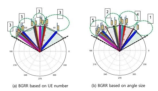
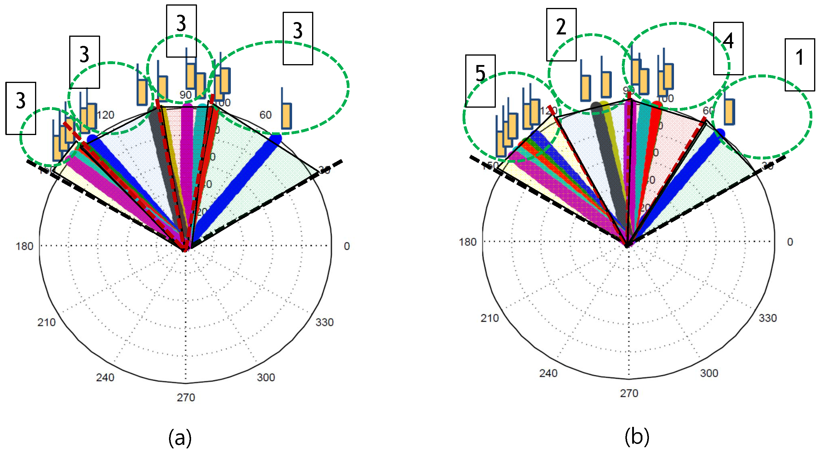
Figure 3 conceptually shows the two cases of sparse UE scenario, when the number of group, ${\upsilon }_{BGRR}=4$. The parameters for the figures are $N_t=100,K=12$. As shown in Figure 3a, in the given 120 degree cell, all of the groups have the same UEs, i.e., three UEs. It should also be noted that the angles of sectors/groups are different. As shown in Figure 3b, all of the groups have the same angle, 30 degrees, but the number of UEs in each angle is different, i.e., 5, 2, 4, 1.

The second scenario is a dense UE distribution (DUD) scenario. If there are too many UEs in a cell, it is impossible to co-schedule and serve all of the UEs in the cell. In this case, we can choose part of the UEs that have favorable channel conditions for signal transmission/reception.

Figure 4 shows the DUD scenario. Since there are a lot of UEs, we only choose three that have favorable channel conditions in each group, and angles are also decided with even 30 degree angles.

Figure 5 shows the reduction of overhead of RS by the proposed BGRR scheme. Assuming each group has the same number of UEs, the expected overhead of RS with the proposed scheme can be derived as follows:

$$\begin{array}{ccc}\hfill {\chi }_{WC{R}_{BGRR}}(\%)& =& ({\eta }_{CRS}+(K+K·{\chi }_{DM-RS})/{\upsilon }_{BGRR})/{\eta }_{R{B}_{tot}}\times 100,\hfill \end{array}$$

(9)

$$\begin{array}{ccc}\hfill {\chi }_{WOC{R}_{BGRR}}(\%)& =& ({\eta }_{CRS}+(N_t+K·{\chi }_{DM-RS})/{\upsilon }_{BGRR})/{\eta }_{R{B}_{tot}}\times 100.\hfill \end{array}$$

(10)

Here, we assume that the CRS is irreducible for backward compatibility, cell search and initial acquisition, etc. All of the other RSs are reducible by the reuse of resource with the BGRR scheme. As shown in Figure 5, the overhead of RS can be significantly reduced with the proposed scheme. Note that the overhead of RS is less than $35\%$, which is definitely acceptable as a system operation point of view, even with $N_t=600$.

In the case of the same size of angles, (9) and (10) can be expressed as follows:

$$\begin{array}{ccc}\hfill {\chi }_{WC{R}_{BGRR}}(\%)& =& ({\eta }_{CRS}+K_{g_{max}}+K_{g_{max}}·{\chi }_{DM-RS})/{\eta }_{R{B}_{tot}}\times 100,\hfill \end{array}$$

(11)

$$\begin{array}{ccc}\hfill {\chi }_{WOC{R}_{BGRR}}(\%)& =& ({\eta }_{CRS}+N_t+K_{g_{max}}·{\chi }_{DM-RS})/{\eta }_{R{B}_{tot}}\times 100,\hfill \end{array}$$

(12)

where $K_{g_{max}}$ is the maximum number of UEs in the fixed angle groups. Note that the number of UEs in each group is different and therefore the RS resource is dependent upon the maximum number of UEs for the case of the same size of angles.

Now, let us show how the proposed scheme can be realized. Figure 6 shows an example of using the BGRR algorithm.

The LS-MIMO only can be used for the static or nomadic UEs due to the burden of the RS overhead. In this regard, the BGRR is also valuable for the static or nomadic UEs. To use the proposed BGRR, we should first know the UE locations to guarantee the space separability among different groups. There are many positioning schemes, and the 3GPP standard already provides the LTE Positioning Protocol (LPP) and continuously trys to improve it. High precision GPS or long-term RS also can be helpful for this. If the rough UE locations are recognized, the virtual sectors can be determined for high beam separability. We can use the UE based or the angle based selection as mentioned previously. Based on the location information, we can generate beams using location based precoding. With the location based precoding, we can send RS or short-term RS to get the channel information. Obviously, the short-term RS resources should be orthogonal with each other in a virtual sector, but can be reused for different sectors. In the case of the WCR, UEs can send the sounding reference signals, and RX beamforming can be used at the BS. After CSI acquisition, the location and the inter-user interference (IUI) reduction precodings are used together to send the data signal. More details will be shown in the following section.

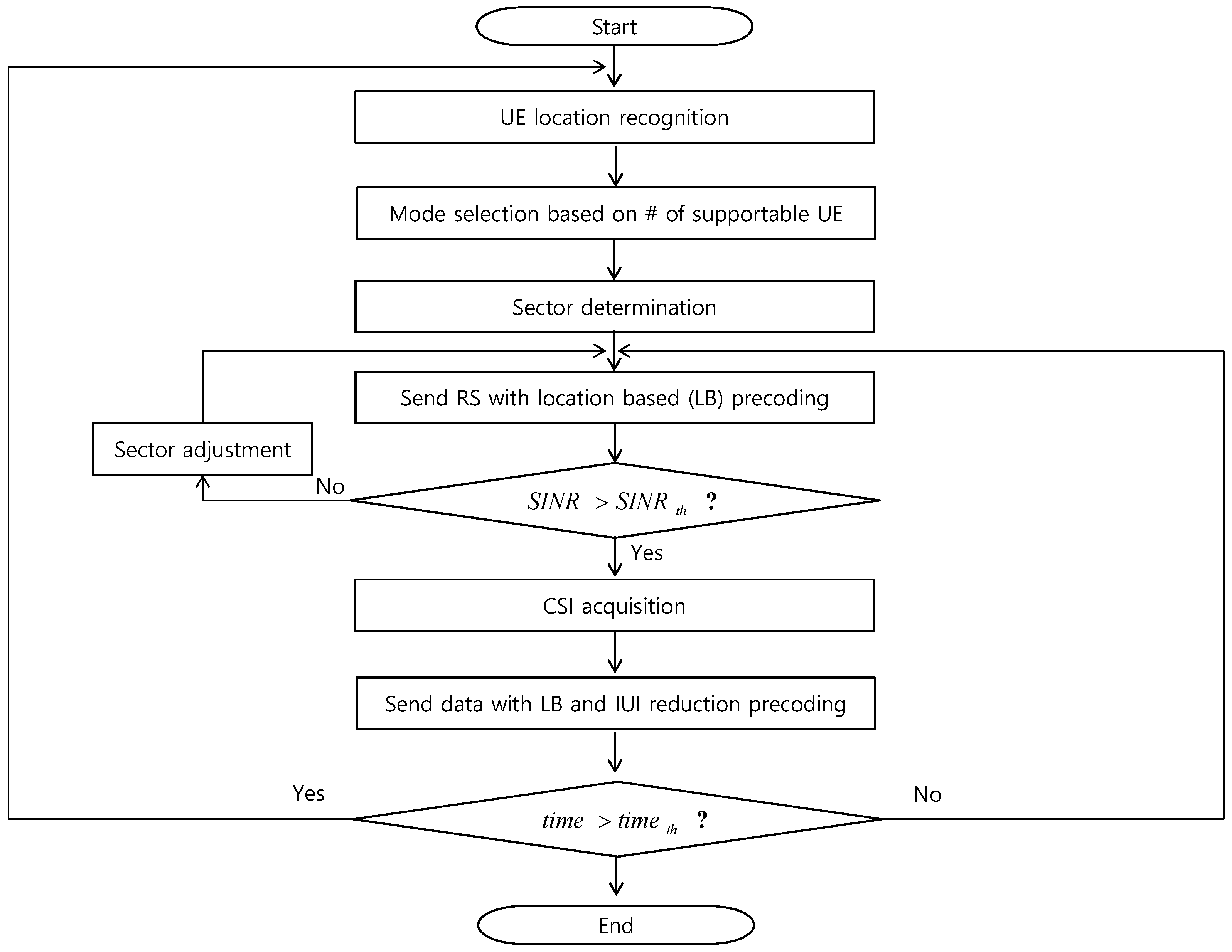
There could be many modifications to improve the BGRR. As one example, we can increase beam separability among groups by using a iterative solution. The flow chart of this example is shown in Figure 7. In this flow chart, we can see that if SINR is not in the satisfactory region, we can adjust the virtual sectors to increase SINR, which can guarantee the high space separability.

5. Numerical Results

In a downlink LS-MIMO system with $N_t$ TX antennas and K single antenna RXs, the $K\times 1$ received signal vector at the UEs can be represented as follows:

$$\mathbf{y}=\sqrt{{\rho }_t}\zeta \mathbf{HDWx}+\mathbf{z},$$

(13)

where ζ is the normalized factor to make total TX power as ${\rho }_t$, $\mathbf{H}$ is the $K\times N_t$ correlated channel matrix that was introduced in Section 2.2, and $\mathbf{D}$ is the precoding matrix for transmit steering matrix, i.e., $\mathbf{D}={[{\mathbf{a}}^H\left(\overline{{\theta }_1}\right),\cdots ,{\mathbf{a}}^H\left(\overline{{\theta }_k}\right),\cdots ,{\mathbf{a}}^H\left(\overline{{\theta }_K}\right)]}^H$, $\overline{{\theta }_k}$ is the average of angular spread, $\mathbf{W}$ is the group precoding matrix, which can be zero-forcing (ZF) or matched filtering (MF) in each group. With the precoding matrix, $\mathbf{H}·\mathbf{D}$ can be represented as follows:

$$\begin{array}{ccc}\hfill \mathbf{H}·\mathbf{D}& =& \left(\begin{array}{c}{\mathbf{g}}_1{\mathbf{A}}_1\hfill \\ {\mathbf{g}}_2{\mathbf{A}}_2\hfill \\ ⋮\hfill \\ {\mathbf{g}}_i{\mathbf{A}}_i\hfill \\ ⋮\hfill \\ {\mathbf{g}}_K{\mathbf{A}}_K\hfill \end{array}\right)·\left({\mathbf{a}}^H\left(\overline{{\theta }_1}\right){\mathbf{a}}^H\left(\overline{{\theta }_2}\right)\cdots {\mathbf{a}}^H\left(\overline{{\theta }_i}\right)\cdots {\mathbf{a}}^H\left(\overline{{\theta }_K}\right)\right),\hfill \\ & =& \left(\begin{array}{c}{\mathbf{g}}_1{\mathbf{A}}_1{\mathbf{a}}^H\left({\overline{\theta }}_1\right){\mathbf{g}}_1{\mathbf{A}}_1{\mathbf{a}}^H\left({\overline{\theta }}_2\right)\cdots {\mathbf{g}}_1{\mathbf{A}}_1{\mathbf{a}}^H\left({\overline{\theta }}_i\right)\cdots {\mathbf{g}}_1{\mathbf{A}}_1{\mathbf{a}}^H\left({\overline{\theta }}_K\right)\hfill \\ {\mathbf{g}}_2{\mathbf{A}}_2{\mathbf{a}}^H\left({\overline{\theta }}_1\right){\mathbf{g}}_1{\mathbf{A}}_2{\mathbf{a}}^H\left({\overline{\theta }}_2\right)\cdots {\mathbf{g}}_2{\mathbf{A}}_2{\mathbf{a}}^H\left({\overline{\theta }}_i\right)\cdots {\mathbf{g}}_2{\mathbf{A}}_2{\mathbf{a}}^H\left({\overline{\theta }}_K\right)\hfill \\ ⋮⋮\ddots ⋮\hfill \\ {\mathbf{g}}_K{\mathbf{A}}_K{\mathbf{a}}^H\left({\overline{\theta }}_1\right){\mathbf{g}}_K{\mathbf{A}}_K{\mathbf{a}}^H\left({\overline{\theta }}_2\right)\cdots {\mathbf{g}}_K{\mathbf{A}}_K{\mathbf{a}}^H\left({\overline{\theta }}_i\right)\cdots {\mathbf{g}}_K{\mathbf{A}}_K{\mathbf{a}}^H\left({\overline{\theta }}_K\right)\hfill \end{array}\right),\hfill \end{array}$$

(14)

By using Label (13) and Label (14), $\mathbf{y}$ can be rewritten as follows:

$$\begin{array}{ccc}\hfill \mathbf{y}& =& \sqrt{{\rho }_t}\zeta \left(\begin{array}{c}{\mathbf{g}}_1{\mathbf{A}}_1{\mathbf{a}}^H\left({\overline{\theta }}_1\right){\mathbf{g}}_1{\mathbf{A}}_1{\mathbf{a}}^H\left({\overline{\theta }}_2\right)\cdots {\mathbf{g}}_1{\mathbf{A}}_1{\mathbf{a}}^H\left({\overline{\theta }}_i\right)\cdots {\mathbf{g}}_1{\mathbf{A}}_1{\mathbf{a}}^H\left({\overline{\theta }}_K\right)\hfill \\ {\mathbf{g}}_2{\mathbf{A}}_2{\mathbf{a}}^H\left({\overline{\theta }}_1\right){\mathbf{g}}_1{\mathbf{A}}_2{\mathbf{a}}^H\left({\overline{\theta }}_2\right)\cdots {\mathbf{g}}_2{\mathbf{A}}_2{\mathbf{a}}^H\left({\overline{\theta }}_i\right)\cdots {\mathbf{g}}_2{\mathbf{A}}_2{\mathbf{a}}^H\left({\overline{\theta }}_K\right)\hfill \\ ⋮⋮\ddots ⋮\hfill \\ {\mathbf{g}}_K{\mathbf{A}}_K{\mathbf{a}}^H\left({\overline{\theta }}_1\right){\mathbf{g}}_K{\mathbf{A}}_K{\mathbf{a}}^H\left({\overline{\theta }}_2\right)\cdots {\mathbf{g}}_K{\mathbf{A}}_K{\mathbf{a}}^H\left({\overline{\theta }}_i\right)\cdots {\mathbf{g}}_K{\mathbf{A}}_K{\mathbf{a}}^H\left({\overline{\theta }}_K\right)\hfill \end{array}\right),\hfill \\ & & \mathbf{W}=\left(\begin{array}{c}{\mathbf{W}}_{{\mathbf{g}}_{\mathbf{1}}}{\mathbf{0}}_{(g_1\times (g_1+g_2+\cdots g_l))}^{}\hfill \\ {\mathbf{0}}_{(g_2\times g_1)}{{\mathbf{W}}_{{\mathbf{g}}_{\mathbf{2}}}}^{}{\mathbf{0}}_{(g_2\times (g_1+g_2+\cdots g_l))}^{}\hfill \\ ⋮\ddots ⋮\hfill \\ {\mathbf{0}}_{(g_l\times (g_1+g_2+\cdots g_{l-1}))}{\mathbf{W}}_{{\mathbf{g}}_{\mathbf{l}}}\hfill \end{array}\right)·\left(\begin{array}{c}{x}_1\hfill \\ x_2\hfill \\ ⋮\hfill \\ x_i\hfill \\ ⋮\hfill \\ x_K\hfill \end{array}\right)+\left(\begin{array}{c}{z}_1\hfill \\ z_2\hfill \\ ⋮\hfill \\ z_i\hfill \\ ⋮\hfill \\ z_K\hfill \end{array}\right),\hfill \end{array}$$

(15)

where ${\mathbf{W}}_{{\mathbf{g}}_{\mathbf{i}}}$ is the precoding matrix for the $i^{th}$ group.

Based on the analysis, spectral efficiency (SE) (bit per second) can be represented as

$$SE=\alpha B·\sum _{i=1}^M\sum _{k=1}^{S_i}E\left[{log}_2\left(1+\frac{{\rho }_t\zeta {\left|{\left(\mathbf{hd}\right)}_k^{g_i}·{\mathbf{w}}_k^{g_i}\right|}^2}{{\rho }_t\zeta {\left|{\displaystyle \sum _{o\ne k}}{\left(\mathbf{hd}\right)}_k^{g_i}·{\mathbf{w}}_o^{g_i}\right|}^2+{\rho }_t\zeta {\left|{\displaystyle \sum _{j\ne i}}{\displaystyle \sum _e}{\left(\mathbf{hd}\right)}_k^{g_i^j}·{\mathbf{w}}_e^{g_j}\right|}^2+N_{0}B}\right)\right],$$

(16)

where α is the scaling factor for the overhead of RS [1], B is the signal bandwidth, M is the total number of groups, $S_i$ is the total number of UEs in $i^{th}$ group, ${\left(\mathbf{hd}\right)}_k^{g_i}$ is the precoded channel vector by using steering vector for $k^{th}$ UE in $g_i^{th}$ group, ${\mathbf{w}}_k^{g_i}$ is the $g_i^{th}$ group precoding vector for $k^{th}$ UE to reduce inter-user interference in the group, and $g_i^j$ is for the indication of the interference signals to the $g_i^{th}$ group after steering precoding (the same rows with $g_i^{th}$ group but different columns in $\mathbf{H}·\mathbf{D}$).

The two interference terms in the denominator of Label (16) are the inter-user interference in a group (${\rho }_t\zeta {\left|{\displaystyle \sum _{o\ne k}}{\left(\mathbf{hd}\right)}_k^{g_i}·{\mathbf{w}}_o^{g_i}\right|}^2$), and the residual interference from steering precoding (${\rho }_t\zeta {\left|{\displaystyle \sum _{j\ne i}}{\displaystyle \sum _e}{\left(\mathbf{hd}\right)}_k^{g_i^j}·{\mathbf{w}}_e^{g_j}\right|}^2$). With Labels (9)–(12), the scaling factor for the overhead of RS is $\alpha =\left(1-\frac{{\chi }_{WC{R}_{BGRR}}}{100}\right)$ for the WCR, and $\alpha =\left(1-\frac{{\chi }_{WOC{R}_{BGRR}}}{100}\right)$ for the WOCR, when the proposed BGRR scheme is applied.

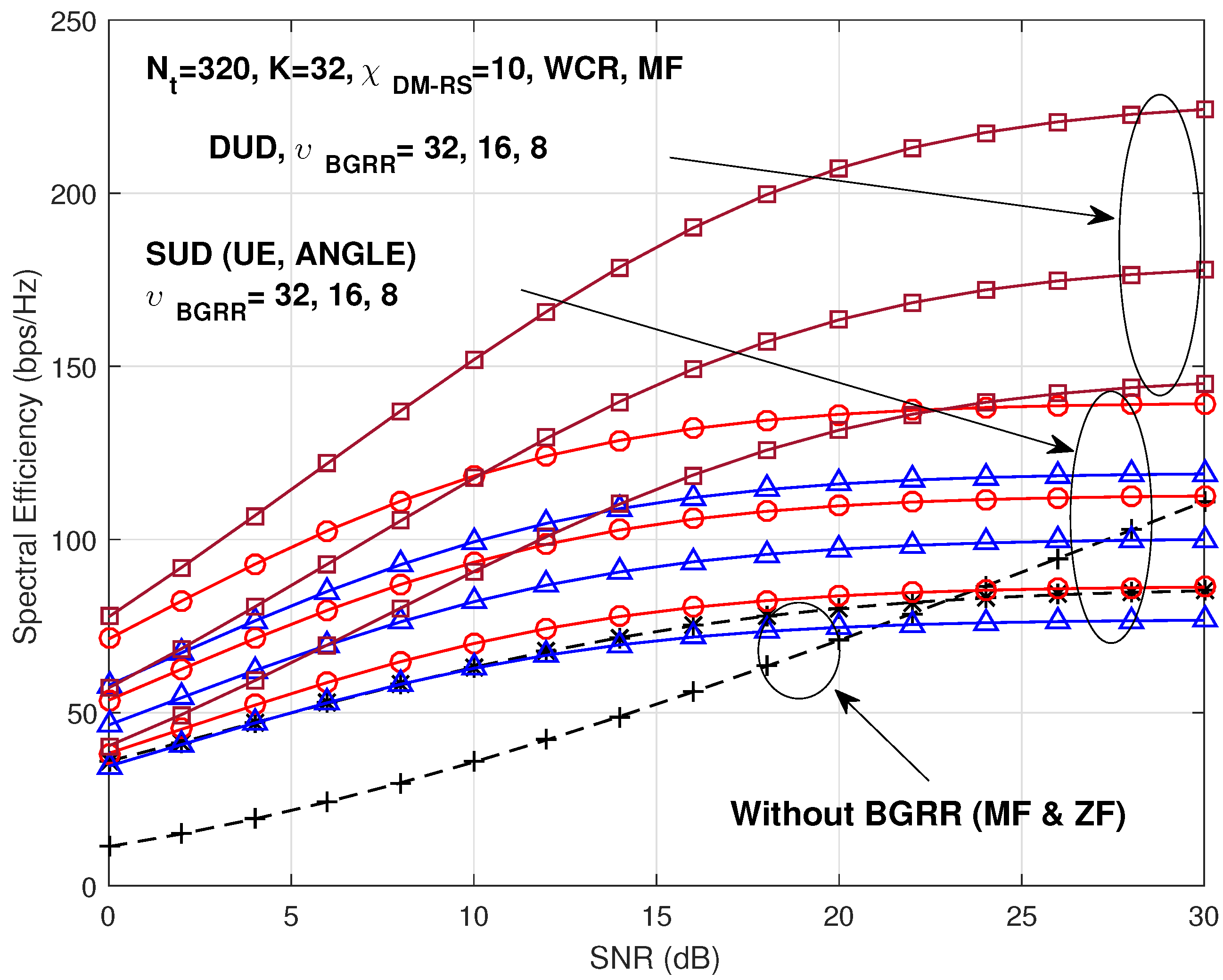
Figure 8 shows the SE (bps/Hz) versus SNR (dB) with $N_t=320,K=32$, ${\chi }_{DM-RS}=10$, ${\upsilon }_{BGRR}=32,16,8$, and MF group precoding. We assume that one cell has a 180-degree angle.

We only show the case of WCR because the case of WOCR would show the similar characteristics, while it gives more improvement of performance with the proposed BGRR scheme. In the case without the BGRR scheme, the number of TX antennas is limited to 273 as shown in the previous section. It is obvious that the DUD gives better performance than the SUD. In the case of the SUD, the UE based grouping scheme (red solid line with ‘O’ marks) shows better performance than the angle based grouping scheme (blue solid ‘△’ marks). Note that the distribution of UEs is not even and MF cannot remove the interference completely in the angle based grouping scheme. Some of the groups could have a lot of UEs and the inter-user interference due to the MF precoding can result in performance loss.

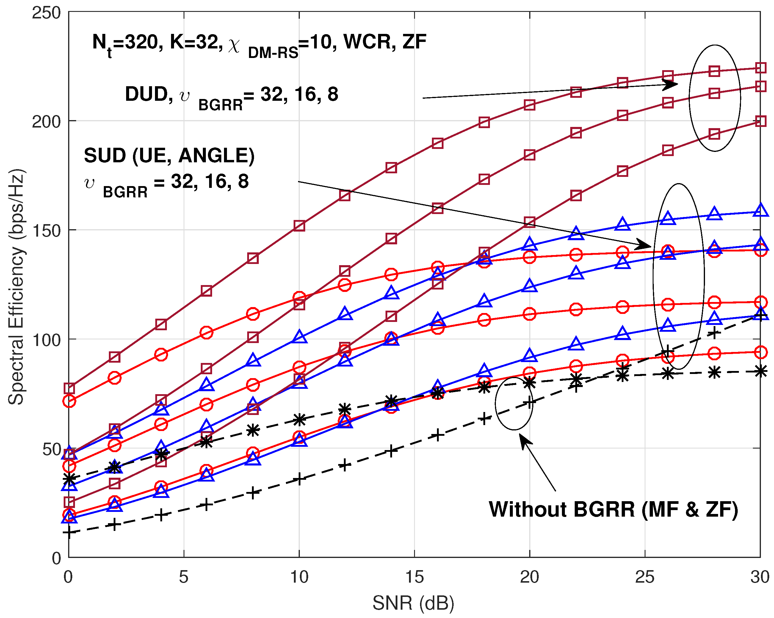
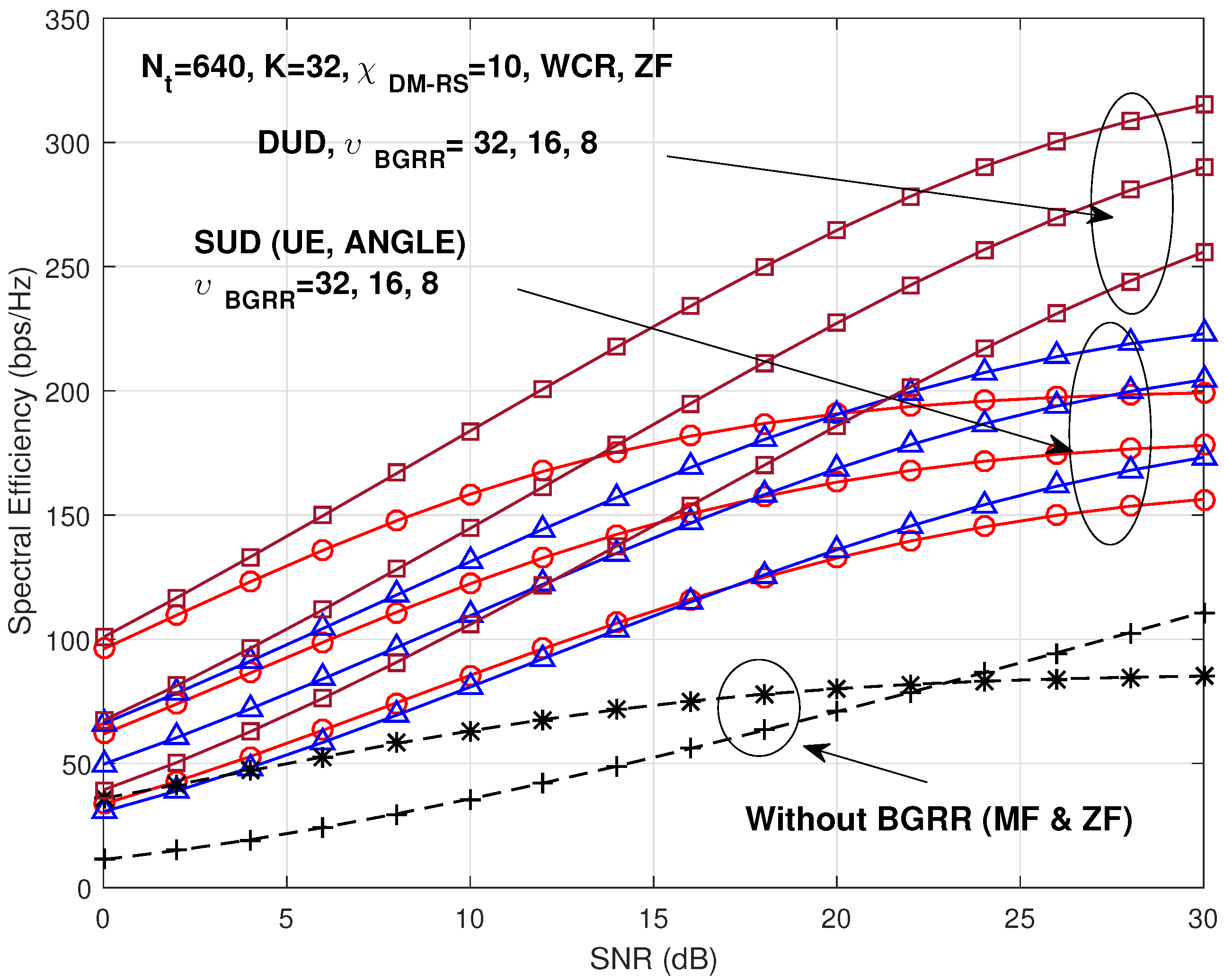
Figure 9 shows the SE (bps/Hz) versus SNR (dB) performance, when the ZF group precoding is used with the same parameters in Figure 8.

As shown in the figure, the performance is different in the case of SUD. In the high SNR region, especially, the performance of the angle based grouping scheme is superior to that of the UE based grouping scheme. This is due to the fact that ZF is near optimum in the high SNR region and can remove inter-user interference completely, even when more UEs are in the same group. In the case of UE based grouping scheme, all of the groups have the same UEs, which means that group angle can be very small, and it causes bad channel conditions. This means that, to get enhanced performance, we should choose between UE based grouping and angle based grouping schemes depending on the situations. Note that the performance trend is maintained as the number of TX antennas and/or UEs is increased.

Figure 10 and Figure 11 show the same case with Figure 8 and Figure 9 except that the number of TX antenna is increased from 320 to 640. The trend is the same as the previous case, but the performance difference between “with BGRR” and “without BGRR” becomes more than the previous case due to higher beamforming effect.

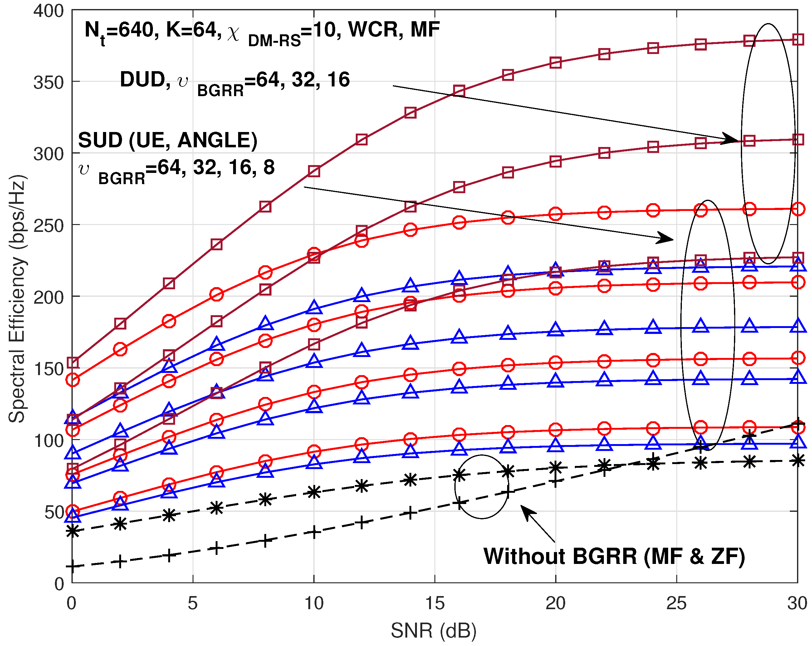
Figure 12 and Figure 13 show the same case as Figure 10 and Figure 11 except that the number of UEs is increased from 32 to 64. As shown in the figures, the trend is also similar with the previous cases.

Since the LS-MIMO is usually used for the DUD case, we can expect drastic performance gain by the proposed BGRR scheme. From Figure 12 and Figure 13, the expected improvement of performance is $444.7\%(85\to 378$ (bps/Hz)) in the case of the MF group precoding scheme, and $340.5\%$ ($111\to 378$ (bps/Hz)) in the case of the ZF group precoding scheme.

As another analysis, we present the case of the channel estimation error of the sounding reference signals. We model the estimated channel as follows:

$$\widehat{\mathbf{H}}=\xi \mathbf{H}+\sqrt{1-{\xi }^2}\mathbf{E},$$

(17)

where $\widehat{\mathbf{H}}$ is the estimated channel matrix, $\xi \in [0,1]$ is the error factor which reflects the degree of channel estimation error, and $\mathbf{E}\in {\mathbb{C}}^{K\times N_t}$ is the error matrix with the same statistical characteristic but independent of the channel. We can get the SE performance in the case of the channel estimation error of the sounding reference signal, if we make a precoding matrix using Label (17), and put the precoding matrix in Label (16).

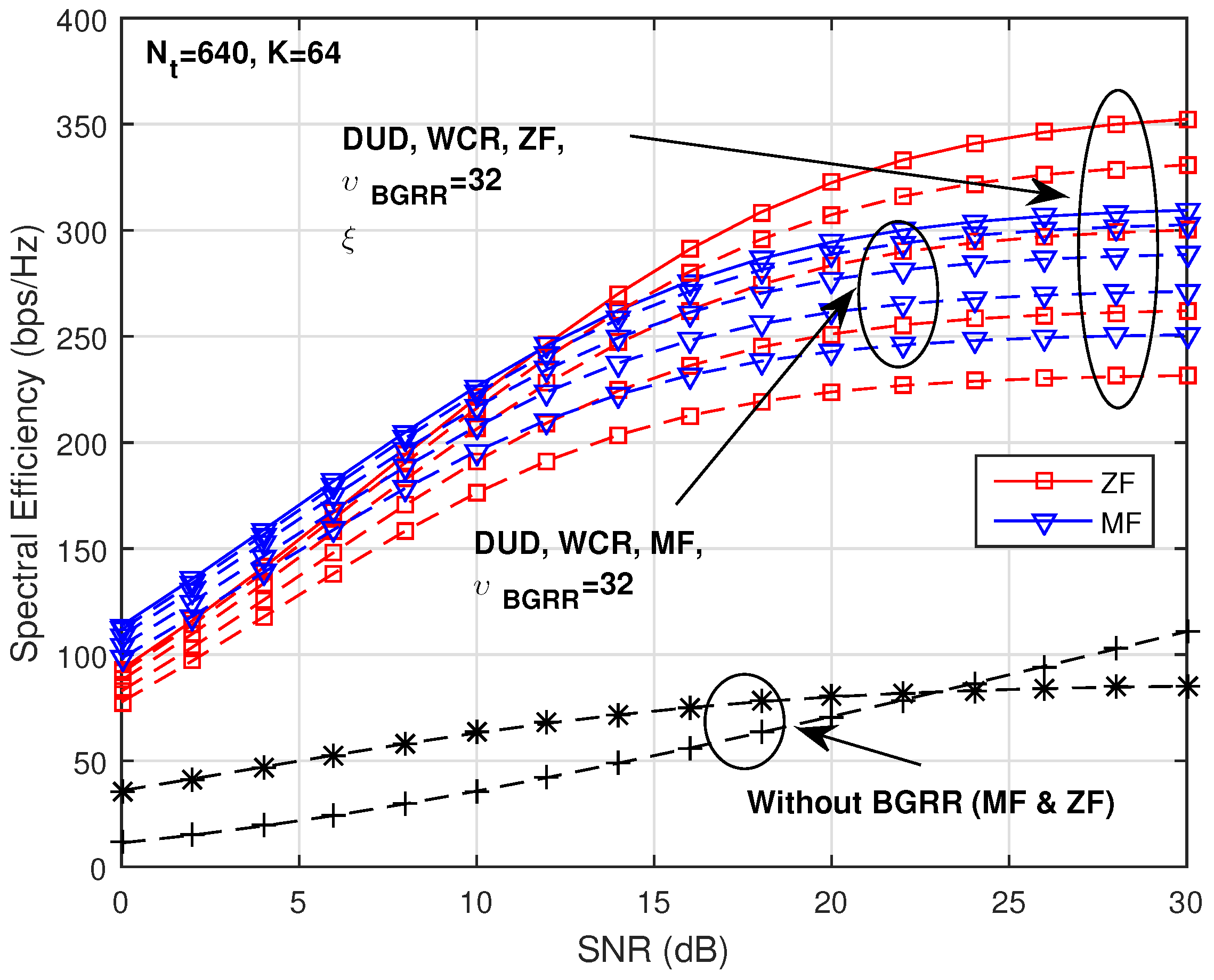
Figure 14 shows the simulation results of SE when the channel estimation error factors are $\xi =1,0.98,0.95,0.90,0.85$. As observed, even when the case of the channel estimation error is very severe ($\xi =0.85$), the performance of the proposed scheme is much better than the conventional one. This means that the proposed scheme is still effective even when there is severe channel estimation error.

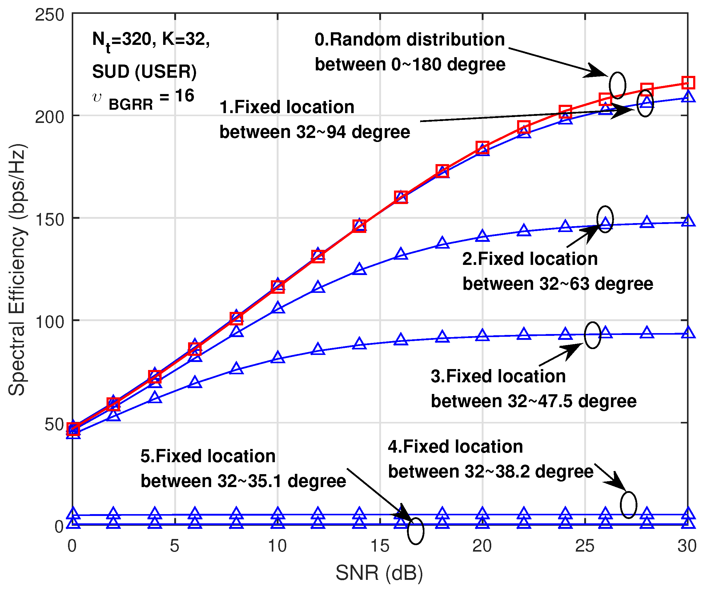
As a last analysis, we present the SE performance based on the space separations among UEs for understanding the characteristics of the proposed scheme.

In Figure 15, we reduce the sector angle to reduce the space separability in the case of 1. Fixed location between 32 and 94 degrees—we locate each user with two-degree separation, in the case of 2. Fixed location between 32 and 63 degrees—we locate each user with one-degree separation, in the case of 3. Fixed location between 32 and 47.5 degrees—we locate each user with 0.5 degree separation, in the case of 4. Fixed location between 32 and 38.2 degrees—we locate each user with 0.2 degree separation, in the case of 5. Fixed location between 32 and 35.1 degrees—we locate each user with 0.1 degree separation.

It is obvious that if a cell angle is reduced, the SE performance is reduced due to the reduction of beam separability among the different virtual sectors. Therefore, for the better performance of the proposed scheme, it is better to choose a wide angle of the cell.

6. Conclusions

In this paper, the RS overhead problem is analyzed, and we proposed a BGRR scheme for the reduction of RS overhead in LS-MIMO systems. We first analyzed the RS overhead in the LS-MIMO system by using the RS overhead model based on the 3GPP LTE-A standard, and provided the performance improvement of the proposed BGRR scheme for two scenarios, sparse UE distribution and dense UE distribution. The dense UE distribution scenario provides more benefits than the sparse UE distribution scenario, due to the multi-UE selection gain. In the sparse UE distribution scenario, we can choose between UE based grouping and angle based grouping schemes because the improvement of performance depends on the situation. We validated that the proposed scheme can remarkably increase spectral efficiency, and could be a core technology for the realization of LS-MIMO systems.