Laplace Domain Boundary Element Method for Structural Health Monitoring of Poly-Crystalline Materials at Micro-Scale

Abstract

This paper describes, for the first time, the application of an Elastodynamic Boundary Element Method (BEM) in Laplace Domain for the Structural Health Monitoring (SHM) of poly-crystalline materials. The study focuses on Ultrasonic Guided Wave (UGW) propagation and investigates the wave–material interactions at micro-scale. The study aims to investigate the interaction of UGWs with assessing micro-structural features such as grain size, morphology, degradation, and flaws. Numerical simulations of the most common micro-structural features demonstrate the accuracy and validity of the proposed method. Particular attention is paid to the study of porosity and its influence on material macro-properties. Different crystal morphologies such as cubic, rhombic, and truncated octahedral are considered. The detection of voids based on the changes in the amplitude and Time of Arrival (ToA) of the backscattered signal is investigated. The study also considers inter-granular cracks, which cause laceration, and examines flaw position/orientation, length, and distance from a specific reference. Furthermore, a framework is proposed for generating Probability of Detection (PoD) curves using numerical simulations. Experimental tests in pristine conditions are shown to be in good agreement with the numerical simulations in terms of ToA, signal amplitude, and wave velocity. The numerical simulations provide insights into wave propagation and wave–material interactions, including different types of defects at the micro-scale. Overall, the BEM and UGW methods are shown to be effective tools for better understanding micro-structural features and their influence on the macro-structural properties of poly-crystalline materials.

1. Introduction

Poly-crystalline materials [1] are commonly used in many engineering structures as they are able to resist severe environmental conditions thanks to their high mechanical and thermal properties. The poly-crystalline structure at the micro-scale is characterized by the random spatial distribution of crystals, also known as grains. Defects such as inter-granular cracks, which occur on the grain boundary; trans-granular cracks, which occur inside the grain; and voids/pores, which lead to porosity often, decrease the material properties of the structure and are the main cause of failure at macro-scale. To improve macroscopic properties of such materials from their design phase up to their potential failure, it is essential to analyze and inspect microscopic features [2]. Structural Health Monitoring (SHM) using Ultrasonic Guided Waves (UGWs) can be an effective technique for detecting micro flaws in poly-crystalline materials. SHM [3,4,5] is an advanced form of Non-Destructive Testing (NDT) used to assess the reliability and safety of components. SHM is the process of monitoring the state of an engineering structure through the response of permanently integrated sensors to detect any changes in the state of the structure. The structure is analyzed, localized, and predicted in a way that NDT becomes an integral part of the structure [6,7]. UGWs are acoustic waves that are generated if the characteristic frequency exceeds a certain threshold (typically above 20 [kHz]), and they propagate through various structures such as plates, sheets, and tubes [8]. The UGW technique is well suited in the SHM framework because the waves undergo absorption or scattering when they encounter the boundaries of a structure or the surfaces of flaws, such as cracks or voids/pores. By determining the velocity of the propagating wave and calculating the time it takes for the scattered or reflected wave to travel, it becomes possible to identify the boundaries of the structure or defects [8,9]. Therefore, utilizing wave–material interactions is possible to characterize material properties, as well as to detect and localize defects in poly-crystals in the NDT-SHM framework [10,11,12]. However, because of the experimental challenges in acquiring detailed information about micro-structure architecture and defect characterization, different numerical and computational methods have been proposed to represent the randomness of the micro-structure and the presence of defects in poly-crystalline materials [1,2,13,14,15]. In recent years, various numerical methods based on elastodynamics theory have been used to study wave propagation and scattering. These methods include the Finite Element Method (FEM) [16,17], Finite Difference Method (FDM) [18,19,20], Finite Volume Method (FVM) (also known as Finite Integration Technique (FIT) [21]), and Boundary Element Method (BEM) [9,22]. Studies have shown that ultrasonic scattering or attenuation can be used to characterize poly-crystalline micro-structures and to localize flaws [17,23,24]. Establishing the relationship between ultrasonic scattering/attenuation and material parameters enables reliable and high-quality material testing [25,26]. The FEM has been used to model wave–material interactions in poly-crystalline materials [11,20,25,26,27]. However, FEM presents limitations. Indeed, it is often difficult to embed inter-granular and trans-granular cracks, voids/pores, and other influential features. Furthermore, the computational expense associated with utilizing FEM to model cracks and voids is significant because of the necessity of employing a fine mesh. Additionally, accurate results necessitate a substantial number of elements per wavelength for high-frequency waves. Another method, the FDM, discretizes elastodynamic equations on a staggered grid but suffers from accuracy issues [20,28]. In contrast, the BEM has gained significance in SHM assessment. BEM provides a more efficient alternative to previous numerical techniques for modeling grain boundaries and the reflection of UGWs. This is because of its ability to discretize solely the boundaries of the micro-structure and the flaws, thereby requiring fewer elements to accurately represent the UGWs [2,29,30]. This study presents the development of the multi-region Elastodynamic BEM in the Laplace Domain to investigate the effects of defects, material properties, and grain variations on wave propagation. The focus of this work is to characterize poly-crystalline materials with the application of the BEM as a tool through which to help, guide, and direct Non-Destructive Testing, such as SHM (see Figure 1).

The main idea of this work is to establish a numerical tool/model based on the BEM for the SHM of poly-crystalline structures with these specific aims and objectives:

• To develop a computational framework for modeling dynamic waves propagation in poly-crystalline materials;
• To investigate the influence of grain morphology, size, and distribution;
• To investigate the possible scattering of UGWs due to the formation of voids and cracks;
• To assess the applicability of this computational framework when utilized to conduct the SHM of poly-crystalline materials.

The characterization of poly-crystalline materials with the application of the BEM has the following advantages:

• Aids in improving and better understanding wave–material interactions and the material micro- and macro-scale features, including random defects (those that are very difficult or impossible to assess with experiments);
• Developing numerical models can lead to reducing the number of experiments; hence, reducing cost and time;
• Numerical models being used to complement experiments to investigate micro-structural features can possibly improve the safety and lifespan of engineering structures in aerospace, oil and gas, and power plant fields.

To demonstrate the accuracy and validity of the proposed method, numerical simulations were carried out and the results are presented, thereby taking into consideration the most common micro-structural features present in poly-crystals and how to detect them. The porosity (presence of voids) was investigated both quantitatively and qualitatively. Different crystal morphologies were considered such as cubic, rhombic, and truncated octahedral. The influence of the volume fraction of porosity on the material macro-properties was analyzed. Furthermore, the detection of voids was considered based on the amplitude and the Time of Arrival (ToA) of the signal that was backscattered by the void itself. Inter-granular cracks that cause the embrittlement of micro-structures lead to a phenomenon called laceration. Thus, it is of high interest to be able to model their failure mechanisms and, consequently, the UGWs’ material interactions. For this reason, parametric analyses were conducted studying three main effects: the position/orientation of the cracks, the length of the crack, and the crack distance from a specific reference. All the effects were examined considering the amplitude and the ToA of the signal that was backscattered by the crack itself. The structure of the paper is as follows: Section 1 outlines a brief introduction to the research field and some fundamental concepts, such as SHM, UGWs, and the types of defects that can be found in poly-crystalline materials. Section 2 explains the methodology/mathematical model implemented (a focus on the BEM and the Elastodymanic BEM, Voronoi tessellation, and implementation of missing grains). Subsequently, Section 3 is dedicated to the numerical results (pristine condition, damaged condition, comparison of BEM-FEM, and Probability of Detection (PoD) analysis). That section then concludes with a comparative analysis between the experimental tests (in pristine condition) and the numerical simulations in order to validate the effectiveness and accuracy of the employed numerical method. Section 4 outlines the conclusions. The paper then ends with the acknowledgments, Appendix A, and references.

2. Materials and Methods

In this section, the generation and discretization of the artificial micro-structures into grain boundary elements is described briefly. Each grain is considered as a single crystal with a random location, morphology, and material orientation.

2.1. Elastodynamic Boundary Integral Equation (BIE) in the Laplace Transform Formulation

The Boundary Element Method (BEM) is an established method for a range of problems in solid mechanics, including fracture and elastic wave propagation problems [2,22,29,31,32]. The BEM requires only the discretization of the boundaries without discretizing the domain. For poly-crystalline materials, only the external domains and grain boundaries need to be discretized, thus reducing the size of the problem substantially in comparison to domain-type methods [30,33,34,35,36]. In the context of a homogeneous and isotropic linear elastic body that is within the spatial domain $\Phi$ and bounded by the boundary $\Sigma$, and when subjected to dynamic forces, let us consider the scenario where initial displacements, velocities, and body forces are all assumed to be zero. Under the assumption of small displacement theory, the Laplace transform of the governing equation for a specific point $\mathbf{x}$ within the body can be expressed as follows:

$$(c_1^2-c_2^2){\overline{u}}_{i,ij}\left(\mathbf{x},s\right)+c_2^2{\overline{u}}_{j,ii}\left(\mathbf{x},s\right)=s^2{\overline{u}}_i\left(\mathbf{x},s\right),$$

(1)

where $c_1$ and $c_2$ are the velocities of longitudinal and shear waves, respectively. ${\overline{u}}_i\left(\mathbf{x},s\right)$ is the component of the transformed displacement of a point $\mathbf{x}$ and s is the Laplace parameter. The displacement of a point ${\mathbf{x}}^{\prime }$ can be determined from the transformed dynamic equivalent of Somigliana’s identity [30,33,34,35,36]:

$$C_{ij}\left({\mathbf{x}}^{\prime }\right){\overline{u}}_j\left({\mathbf{x}}^{\prime },s\right)={\int }_{\Sigma }{\overline{U}}_{ij}\left({\mathbf{x}}^{\prime },\mathbf{x},s\right){\overline{t}}_j\left(\mathbf{x},s\right)d\Sigma \left(\mathbf{x}\right)-{⨍}_{\Sigma }{\overline{T}}_{ij}\left({\mathbf{x}}^{\prime },\mathbf{x},s\right){\overline{u}}_j\left(\mathbf{x},s\right)d\Sigma \left(\mathbf{x}\right)fori,j=1,2,$$

(2)

where ${\overline{u}}_j\left(\mathbf{x},s\right)$ and ${\overline{t}}_j\left(\mathbf{x},s\right)$ are the Laplace transform of the displacement and tractions, respectively. At the boundary, ${\overline{U}}_{ij}\left({\mathbf{x}}^{\prime },\mathbf{x},s\right)$ and ${\overline{T}}_{ij}\left({\mathbf{x}}^{\prime },\mathbf{x},s\right)$ are the Laplace transform of the fundamental solutions of elastodynamics (they are given in Appendix A). ${\mathbf{x}}^{\prime }$ is the collocation point, which can be a domain or a boundary point; $\mathbf{x}$ is the integration point (boundary point); and $C_{ij}\left({\mathbf{x}}^{\prime }\right)$ is a constant, depending on the position of the collocation point. The spatial variation of the transformed boundary displacements and tractions was approximated by dividing the boundary $\Sigma$ into $N_e$ boundary linear elements, and the variation of boundary values was approximated using constant elements. Hence, the discretized form of Equation (2) is as follows:

$$C_{ij}\left({\mathbf{x}}^{\prime }\right){\overline{u}}_j\left(s\right)=\sum _{n=1}^{N_e}\left[{\overline{t}}_j^n\left(s\right){\int }_{-1}^1{\overline{U}}_{ij}\left(\mathbf{x}\left(\eta \right),s\right)J^n\left(\eta \right)d\eta -{\overline{u}}_j^n\left(s\right){\int }_{-1}^1{\overline{T}}_{ij}\left(\mathbf{x}\left(\eta \right),s\right)J^n\left(\eta \right)d\eta \right]$$

(3)

where $J^n\left(\eta \right)$ is the Jacobian of the transformation, and $\eta$ is the local non-dimensional coordinates $(-1\le \eta \le +1)$. The set of boundary equations, applied to all the boundary nodes, can be written in matrix form as follows:

$$\overline{H}\overline{u}=\overline{G}\overline{t}$$

(4)

where $\overline{u}$ and $\overline{t}$ contain the nodal values of the transformed displacement and tractions, respectively. $\overline{H}$ and $\overline{G}$ depend upon integrals of the transformed fundamental solutions, as well as the Jacobian and the interpolating functions. The matrices $\overline{H}$ and $\overline{G}$ were reordered according to the boundary conditions to give the new matrices $\overline{A}$ and $\overline{B}$. The matrix $\overline{A}$ was multiplied by the vector $\overline{x}$ of unknown transformed displacements and tractions, and $\overline{B}$, by the vector $\overline{y}$ of the known transformed boundary conditions, is as follows:

$$\overline{A}\overline{x}=\overline{B}\overline{y}$$

(5)

The system of equations represented by matrix in Equation (5) was solved to determine the unknown transformed displacements and tractions for a specific Laplace parameter. To obtain the unknown displacements and tractions as functions of time, the transformed variables must be computed for a range of Laplace parameters. The numerical inversion of the Laplace transform can be achieved using Durbin’s method, which relies on a Fast Fourier Transform (FFT). The values of a transformed function, denoted as $\overline{f}\left(s\right)$, were calculated for a series of Laplace parameters, denoted as $s_k=a+\frac{i2k\pi }{T}$. Here, a represents a constant, $i=\sqrt{-1}$, and T is the relevant time interval of interest. The values of the original function, denoted as $f\left(\tau \right)$, were obtained at periodic time instances ${\tau }_m=m\Delta t\left(m=1\dots M-1\right)$, as determined by the following equation:

$$f\left({\tau }_m\right)=\frac{2}{T}exp\left(am\Delta \tau \right)\left\{-\frac{1}{2}Re\left[\overline{f}\left(a\right)+Re\left[\sum _{k=0}^{M-1}\left(A\left(k\right)+iB\left(k\right)\right)W^{mk}\right]\right]\right\},$$

(6)

where:

$$\begin{array}{cc}\hfill & A\left(k\right)=\sum _{l=0}^{L}Re\left[\overline{f}(a+i(k+lM)\frac{2\pi }{T}\right]\hfill \\ \hfill & B\left(k\right)=\sum _{l=0}^{L}Im\left[\overline{f}\left(a\right)+i\left(k+lM\right)\frac{2\pi }{T}\right]\hfill \\ \hfill & W=exp\left(i\frac{2\pi }{M}\right),\hfill \end{array}$$

(7)

and $Re\left[\right]$ and $Im\left[\right]$ denote the real and imaginary parts, respectively. To model poly-crystalline materials at micro-scale, the multi-region BEM formulation was developed. Let us consider the micro-structure as shown in Figure 2. Two possible boundaries can be present for each grain $G=1,\dots N_g$, where $N_g$ is the number of grains considered, ${\Sigma }_{nc}^G$ is the green boundary indicating the intersection between the grain and the domain’s boundary (nc = non contact), and ${\Sigma }_c^G$ is the black boundary interface between the adjacent grains (c = contact). Hence, the entire grain boundary is given by the following:

$${\Sigma }^G{=\Sigma }_{nc}^G\bigcup {\Sigma }_c^G.$$

(8)

For each grain, the following variables were defined:

• ${\tilde{u}}_{nc}^G$, ${\tilde{t}}_{nc}^G$ nodal displacements and tractions at the external boundary;
• ${\tilde{u}}_c^G$, ${\tilde{t}}_c^G$ nodal displacements and tractions at the grain–boundary interface.

For each grain, the displacement boundary integral Equation (2) can be written as follows:

$$\begin{array}{cc}\hfill C_{ij}^G\left({\mathbf{x}}^{{}^{\prime }}\right){\tilde{u}}_j^G({\mathbf{x}}^{{}^{\prime }},s)+{⨍}_{\widetilde{{\Sigma }_{nc}^G}}\widetilde{T_{ij}^G}({\mathbf{x}}^{{}^{\prime }},s)\widetilde{u_j^G}\left(x\right)d\widetilde{{\Sigma }_{nc}^G}& +{⨍}_{\widetilde{{\Sigma }_c^G}}\widetilde{T_{ij}^G}({\mathbf{x}}^{{}^{\prime }},s)\widetilde{u_j^G}\left(x\right)d\widetilde{{\Sigma }_c^G}\hfill \\ \hfill ={\int }_{\widetilde{{\Sigma }_{nc}^G}}\widetilde{U_{ij}^G}({\mathbf{x}}^{{}^{\prime }},s)\widetilde{t_j^G}\left(x\right)d\widetilde{{\Sigma }_{nc}^G}& +{\int }_{\widetilde{{\Sigma }_c^G}}\widetilde{U_{ij}^G}({\mathbf{x}}^{{}^{\prime }},s)\widetilde{t_j^G}\left(x\right)d\widetilde{{\Sigma }_c^G},\hfill \end{array}$$

(9)

where the symbol $\left(\widetilde{f_i}\right)$ indicates a quantity expressed in the material reference system. Equation (9) can be written in matrix form:

$$\left[\begin{array}{cc}{\tilde{H}}_{nc}^G& {\tilde{H}}_c^G\end{array}\right]\left\{\begin{array}{c}{\tilde{u}}_{nc}^G\\ {\tilde{u}}_c^G\end{array}\right\}=\left[\begin{array}{cc}{\tilde{G}}_{nc}^G& {\tilde{G}}_c^G\end{array}\right]\left\{\begin{array}{c}{\tilde{t}}_{nc}^G\\ {\tilde{t}}_c^G\end{array}\right\}.$$

(10)

Interface boundary conditions between two adjacent grains “p” and “q” were applied as follows:

$$\begin{array}{cc}\hfill & \delta u^I=u_c^p+u_c^q\hfill \\ \hfill & t^I=t_c^p=t_c^q.\hfill \end{array}$$

(11)

Re-arranging the system with unknowns on the left-hand side and known variables on the right-hand side in a similar procedure as Equation (5) gives the following:

$$\left[\begin{array}{ccc}{\tilde{A}}^p& {\tilde{H}}_I^p& 0\\ \widetilde{A^q}& \widetilde{{-H}_I^q}& \widetilde{H_I^q}\end{array}\begin{array}{c}\widetilde{{-G}_I^p}\\ \widetilde{{-G}_I^q}\end{array}\right]\left\{\begin{array}{c}\tilde{x}\\ {\tilde{u}}^I\\ {\widetilde{\delta u}}^I\\ {\tilde{t}}^I\end{array}\right\}=\left\{\begin{array}{c}{\tilde{B}}^p·\tilde{y}\\ {\tilde{B}}^q·\tilde{y}\end{array}\right\}.$$

(12)

2.2. Artificial Micro-Structure Generation: Voronoi Tessellation

The accurate representation of material grain morphology is crucial for numerically simulating UGWs in poly-crystalline materials. Researchers use imaging methods such as optical and Scanning Electron Microscopy (SEM) to assess grain size, shape, and distribution. Furthermore, artificial micro-structure generation methods can also be used. Regular morphologies like cubic, rhombic, or truncated octahedral grains are suitable for overall material characterizations through homogenization procedures. However, to capture local grain features and predict flaws or local material properties, Voronoi tessellations (VTs) are preferred. VTs are topologically close to poly-crystalline materials (metals and ceramics) [13,14,15] due to their statistical characteristics. VTs represent real structures closely by considering the stochastic effect of each grain’s crystal anisotropy within the entire aggregate. The grains are generated using completely random seed points, thereby exhibiting a log-normal distribution, as observed in real poly-crystalline materials [13,14,15]. A 2D quasi-random generator using Sobol’s sequence [37] was employed as a uniform random point generator. Figure 3 illustrates a randomly generated artificial micro-structure, which was produced using the previously mentioned method. Since the present work considers 2D problems, to maintain the random character of the generated micro-structure and the stochastic effects of each grain on the overall behavior of the system, three different cases were considered for each grain [13]. In Figure 3, each grain color represents the different orientation of each grain. A specific orientation was given randomly to each grain and was characterized by a counterclockwise angle $\theta$, which was measured from the x axis, where $0^{\circ }\le \theta \le {360}^{\circ }$, and this rotates the local coordinate system of each grain to a new position $x_0-y_0$. The number within each grain represents the grain ID number, hence the number 1 means grain 1 and so on.

2.3. Implementation of Missing Grains: Porosity (Voids/Pores)

As previously mentioned in the introduction, poly-crystalline structures are subject to various defects that have a detrimental impact on their material properties. One such defect is voids/pores, which manifest as material porosity. Porosity can arise from various factors, including low-quality manufacturing processes, material treatments, and environmental conditions. Detecting and characterizing porosity is of utmost importance as it significantly diminishes the mechanical properties of a material. Two possible models were available to incorporate voids into the micro-structure:

• Localize the missing grains, as well as completely remove them from the micro-structure and from the calculation of the BE matrices;
• Consider the material elastic properties of the specific missing grain as very small (Young’s modulus and the Poisson ratio tended toward zero) compared with the ones of the other grains.

Although the second modeling option is considerably simpler to implement compared to the first one, it lacks computational efficiency as the system matrix needs to be computed in its entirety. Consequently, there are no advantages in terms of memory allocation and computational time, which is particularly evident when dealing with many grains. Hence, to implement the first modeling option, the subsequent steps were executed in the numerical model:

• After the generation of the micro-structure by utilizing the VT, the locations of the absent grains (pores) were determined and designated with a unique flag to facilitate their identification;
• The calculation of the BE matrices H and G was bypassed for the grains identified with a specific flag, and they were excluded from the population of the ultimate system of equations. This resulted in a consistent reduction in the equation system’s order;
• The boundary interfaces of the grains neighboring the absent ones (pores) were subjected to the imposition of free traction boundary conditions rather than enforcing interface continuity and equilibrium equations.

From a numerical standpoint, when voids are considered, the number of rows and columns of the final system is reduced according to the following:

$$N_p=N_0-4N_i,$$

(13)

where the system order $N_0$ represents the case when no grains have been removed, while $N_i$ corresponds to the number of interface nodes associated with the missing grains. Both proposed porosity models allow for the manipulation of volume fraction, pore size, and the distribution of the porosity, thus enabling simulations of the response of real porous materials to a specified load. Once the porosity model was incorporated into the numerical model, the process of homogenization was employed to derive the material properties based on the constitutive laws and spatial distribution of micro-components within the micro-structure. Homogenization is typically associated with the concept of the Representative Volume Element (RVE). Material homogenization involves evaluating volume and ensemble averages of relevant fields across one or more realizations of the micro-structure under suitable boundary conditions. Subsequently, it then involves connecting these averaged fields using effective properties. Given a poly-crystalline micro-structure $R\left(N_g\right)$ consisting of $N_g$ grains subjected to consistent boundary conditions—where the material is assumed to be free from micro-cracks—stress and strain volume averages were utilized to extract the apparent elastic moduli. To extract the properties at the micro-scale, averaging theorems in micro-mechanics were employed, which was followed by transferring the obtained information to the macro-scale. The volume average of stresses over an RVE volume, when utilizing the divergence theorem, can expressed with the following equation:

$${\overline{\sigma }}_{ij}=\frac{1}{V}{\int }_V{\sigma }_{ij}\left(\mathbf{x}\right)dV\left(\mathbf{x}\right)=\frac{1}{V}{\int }_{\Sigma }{x}_i{t}_{j}d\Sigma ,$$

(14)

where $x_i$ is the $i-th$ component of the position vector of the point lying on the RVE boundary $\Sigma$, i.e., $i\in \Sigma$. The strains could be evaluated instead as follows, where, again, the divergence theorem has been applied:

$${\overline{\epsilon }}_{ij}=\frac{1}{2V}{\int }_V\left(u_{i,j}\left(\mathbf{x}\right)+u_{j,i}\left(\mathbf{x}\right)\right)dV\left(\mathbf{x}\right)=\frac{1}{2V}{\int }_{\Sigma }\left(u_i{n}_j+u_j{n}_i\right)d\Sigma .$$

(15)

It is interesting to highlight here that, in the case of cohesive cracks or internal discontinuities, the average stress was not affected because they were either in equilibrium or traction free, and the stress integral was evaluated only along the external boundary of the domain (RVE). The same simplification did not apply, however, to the strains; therefore, internal discontinuities or decohesions had to be considered explicitly when computing the integrals due to the local displacement jumps $u_i^I$. Hence, the following more general relationship applied:

$${\overline{\epsilon }}_{ij}=\frac{1}{2V}\left\{{\int }_{\Sigma }\left(u_i{n}_j+u_j{n}_i\right)d\Sigma -{\int }_{{\Sigma }^I}\left(\delta u_i^I{n}_j^I+\delta u_j^I{n}_i^I\right)d{\Sigma }^I\right\},$$

(16)

where ${\Sigma }^I$ are the surfaces of the discontinuities and $n_i^I$ the components of their unit normal vectors. Once the stress $\Omega$ and strain $\Gamma$ in the macro-scale were known, the apparent macro-properties could be defined by the following:

$$\Omega =\widehat{C}\Gamma ,$$

(17)

where $\left(\widehat{·}\right)$ denotes macroscopic properties, which are used to distinguish them from the microscopic ones. Equation (17) is the homogenized stress–strain equation, and it forms the basis for the homogenization procedure. The macroscopic properties were computed for each considered micro-structural realization. Hence, under the plane strain assumption, the constitutive equation in Voigt notation was as follows:

$$\left[\begin{array}{c}{\sigma }_{xx}\\ {\sigma }_{yy}\\ {\sigma }_{xy}\end{array}\right]=\frac{E}{\left(1+\upsilon \right)\left(1-2\upsilon \right)}\left[\begin{array}{ccc}1-\upsilon & \upsilon & 0\\ \upsilon & 1-\upsilon & 0\\ 0& 0& 1-2\upsilon \end{array}\right]\left[\begin{array}{c}{\epsilon }_{xx}\\ {\epsilon }_{yy}\\ {\epsilon }_{xy}\end{array}\right],$$

(18)

where E and $\nu$ are the Young’s modulus and Poisson’s ratio, respectively. The volume fraction of porosity $V_f$ (per unit length) is as follows:

$$V_f=\left(\frac{\left(\frac{l_x·l_y}{N_g}\right)·N_{mg}}{l_x·l_y}\right)·100\%,$$

(19)

where $l_x$ and $l_y$ are the x and y dimension of the micro-structure, respectively. $N_g$ is the number of grains and $N_{mg}$ is the number of missing grains. Considering that the stress–strain field ($\Omega$ and $\Gamma$) was obtained by simulations, the only unknown to be evaluated from the system of Equation (17) was the mechanical stiffness matrix (i.e., $\widehat{C}$ where, if needed, the Young’s and Shear moduli can be evaluated).

2.4. Elastodynamic Algorithm for UGW Propagation

The main algorithm of the proposed method for simulating UGW propagation within poly-crystalline materials is illustrated in Figure 4. The algorithm starts by considering the input file where the number (#) of grains, the mean grain area, and the boundary dimensions of the micro-structure can be selected. Then, the micro-structure can be generated by choosing the desired VT algorithm. Furthermore, if necessary, each micro-flaw (e.g., inter-granular crack or void) was modeled and embedded within the micro-structure. After that, the micro-structure was discretized by creating the grain boundary elements mesh, as was explained in the section related to the BEM. The UGWs, of which the user can define the type, amplitude, and center frequency, were modeled in the Laplace domain. The selection of the number of Laplace parameters was pivotal for achieving optimal solution accuracy. It was observed that increasing the number of Laplace parameters leaded to higher solution accuracy. However, this improvement came at the expense of increased computational cost, and the relationship between the number of parameters and computational cost was non-linear. Therefore, it was essential to strike a balance between accuracy and computational cost to find the optimal compromise. Moreover, the structural mesh size needed to be carefully chosen to strike the corretc balance between accuracy and computational cost. Additionally, the time step, which is influenced by the wave frequency, must be appropriately selected. The system of Equations (5) can be solved at this point. Moreover, with a reliable and fast post-processing, the boundary solutions can be computed. Based on data interpretation and processing, the desired outcomes were obtained.

3. Results and Discussion

In this section, the results of the numerical simulations for the case studies listed below are presented and discussed in depth:

• Numerical validation with experimental tests;
• Grain area distributions;
• Multi-region micro-structure for pristine structure using UGWs;
• Benchmark FEM vs. BEM;
• Missing grains (porosity);
• Parametric analysis with inter-granular cracks (debonding);
• Probability of Detection (PoD) with inter-granular cracks.

3.1. Numerical Validation with Experimental Tests

To validate the numerical method, a series of experimental tests were conducted under pristine conditions. The objective was to compare the ToA, signal amplitude, and wave velocity between the numerical and experimental signals.

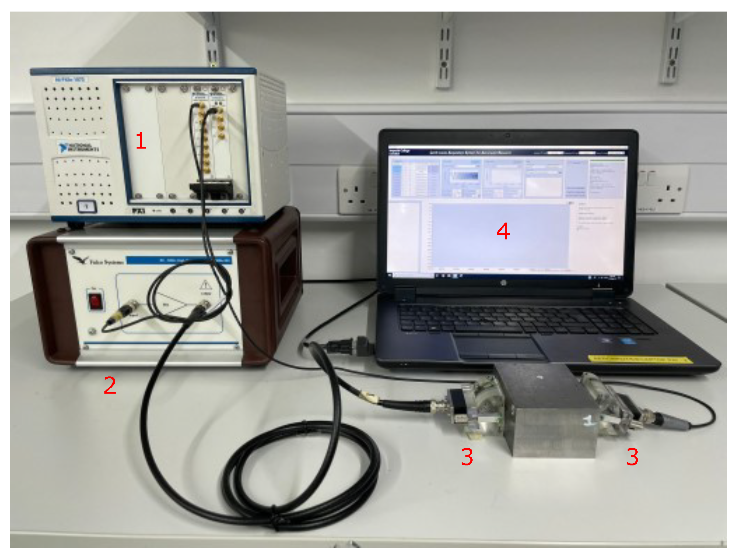
Figure 5 presents a schematic diagram that illustrates the essential components required for an experimental platform that is dedicated to damage detection applications using UGWs. The platform necessitates a minimum of five elements, namely a a signal generator ($No.1$ in the figure), a power amplifier ($No.2$), an acquisition system (i.e., oscilloscope) ($No.1$), one or more transducers ($No.3$), and a personal computer (PC) ($No.4$). Specifically, the experimental step-by-step process from signal generation to acquisition was as follows:

• The signal was generated with a NI-PXI wave generator;
• The actuation signal was amplified using the amplifier module;
• The resulting signal was applied by an Olympus A413S transducer to the specimen to initiate the desired response;
• Another transducer, functioning as a sensor, was employed to capture the resulting signals;
• The signal was acquired via an NI-PXI oscilloscope;
• For data acquisition and manipulation, a PC equipped with dedicated acquisition software was utilized.

A 50 [mV] peak-to-peak amplitude, amplified 50 times by the amplifier with a center frequency of 500 [kHz], was applied with the actuation probe. The sampling frequency was set at 60 [MHz]. The total recording duration for the experimental signals was $t_{tot}=100[\mathsf{\mu }$s], and each measurement was recorded 50 times and averaged to enhance the signal-to-noise ratio. The transducer configuration employed was a pitch–catch arrangement, where the positions of the actuator and sensor were switched to account for the uncertainties based on the measurements, as depicted in Figure 6.

The material under investigation was steel with the dimensions of $l=100$ [mm], $h=50$ [mm], and $w=75$ [mm]. Moreover, the material properties assumed were $E=200$ [GPa], $\nu =0.30$, and $\rho =8000\left[\frac{\mathrm{kg}}{{\mathrm{m}}^3}\right]$ [38].

The micro-structure under investigation consisted of 100 randomly distributed grains with random material orientation. The average grain size was determined to be $ASTMG=10.7\left({\overline{A}}^{gr}=56.25\left[\mathsf{\mu }{\mathrm{m}}^2\right],{\overline{d}}^{gr}=7.5\left[\mathsf{\mu }\mathrm{m}\right]\right)$ [39]. The 2D numerical model used had dimensions of $100\times 75$ [mm${}^2$], as depicted in Figure 7.

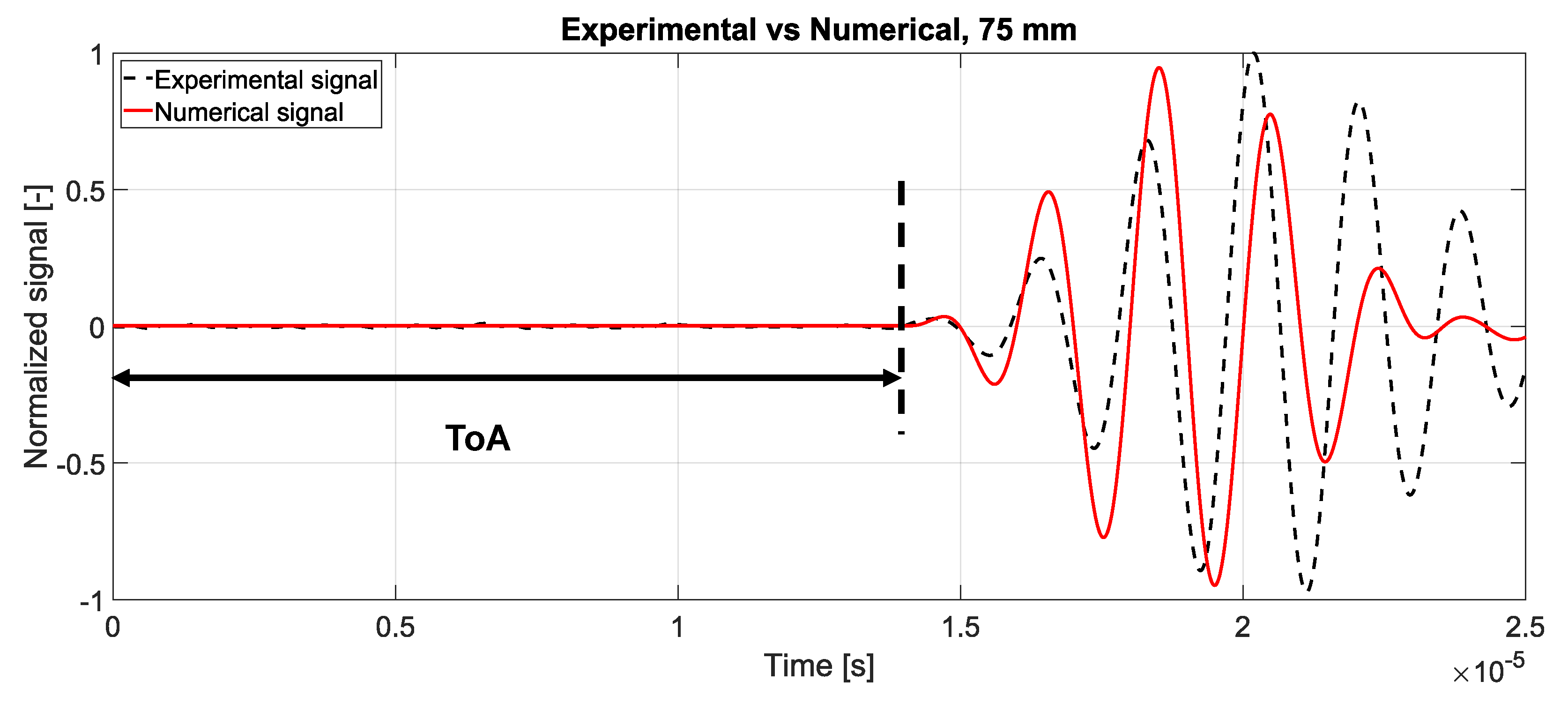
The input signal was defined at the upper edge of the micro-structure, where a prescribed traction of a 5-cycle tone burst with a Hanning window and center frequency of 500 [kHz] was enforced. The resulting signal was acquired at the bottom edge of the micro-structure. The time interval of the simulation was 25 [$\mathsf{\mu }$s] with a time step of 10 [ns] and a time interval of the excitation of 10 [$\mathsf{\mu }$s]. Figure 8 presents a comparative analysis of the experimental and numerical signals that were obtained from a sensor located at a distance of 75 [mm] from the actuator. The comparison revealed a strong agreement between the two sets of results in terms of ToA, amplitude, and wave velocity. Specifically, the experimental ToA value was measured at $13.10[\mathsf{\mu }$s], while the corresponding numerical value was recorded as $13.23[\mathsf{\mu }$s], thus resulting in a small relative error of $0.983\%$. The observed consistency between the experimental and numerical results indicated a reliable correspondence between the physical measurements and the numerical modeling. This agreement in ToA, amplitude, and wave velocity further validated the accuracy and effectiveness of the numerical simulation in capturing the behavior and characteristics of the system under investigation.

3.2. Grain Area Distributions

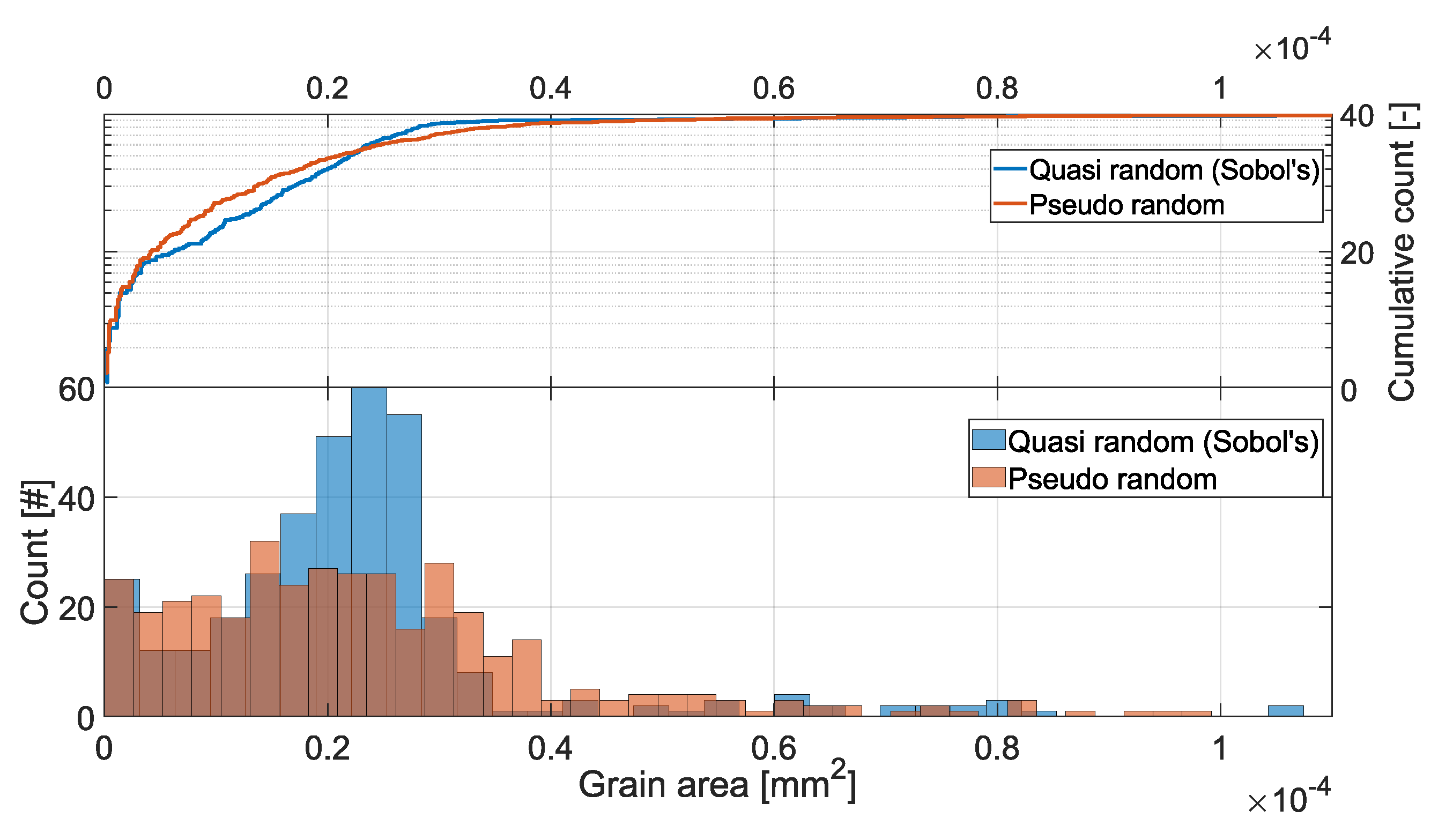
To generate the desired micro-structure, a uniform random point generator was employed. The 2D quasi-random generator (Sobol’s sequence) was chosen. Extensive tests and comparisons were conducted between the quasi-random generator and a pseudo-random point generator. The simulations consistently demonstrated that the quasi-random generator yielded superior grain morphology compared to the pseudo-random generator. Specifically, the quasi-random generator exhibited a higher proportion of equiaxed grains compared to the pseudo-random generator, as evident in Figure 9. Furthermore, the standard deviation of the mean grain area obtained from the quasi-random generator was consistently lower than that of the pseudo-random generator, as depicted in Figure 10.

The mean grain area distribution for different micro-structures was evaluated. Additionally, by employing ImageJ software version 1.53o [40], it was possible to obtain the following:

• A plot of the grain area vs. the # of grains;
• A plot of the grain area vs. the cumulative # of grains.

Figure 10 and Figure 11 present the resulting grain area distribution for a case of 500 grains with an average grain area of $A_{gr}=30.52\times {10}^{-6}$ [mm${}^2$] ($ASTMG=12$ [39]).

3.3. The Multi-Region Micro-Structure for Pristine Structures Using UGWs

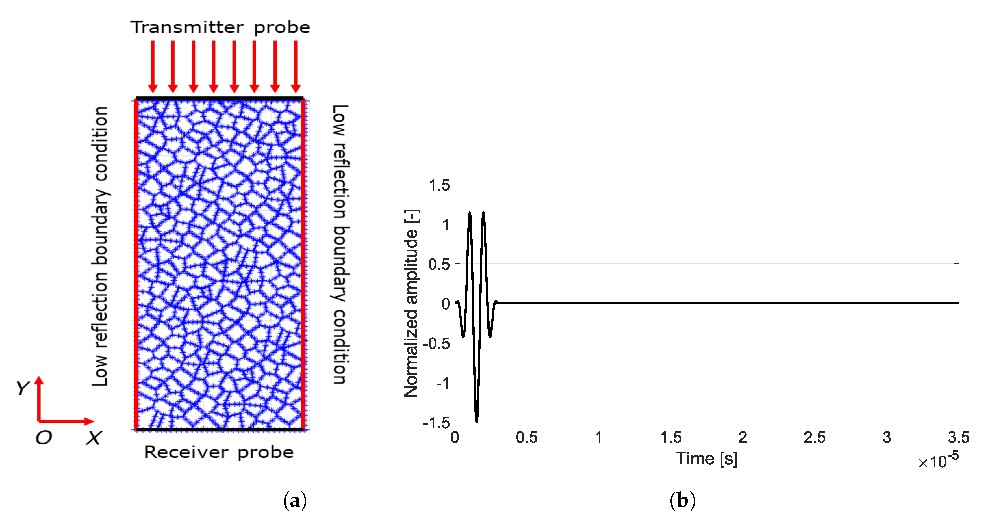
To verify the accuracy of the propagation of UGWs when using the multi-region formulation, a comparison with the homogenized solution was conducted. The homogenized solution was obtained considering only “one” grain (i.e., the micro-structure is a plate with the same external boundaries as the multi-region one). Each grain was characterized by its unique crystallographic orientation and shape. In this comparison, four different numbers of grains were considered, namely 15, 30, 50, and 100. To accurately simulate a 3-cycle toneburst with a center frequency of 1 [MHz], a total of 300 Laplace parameters were employed. The time step used in the simulation was 10 [ns], while the time window for the entire simulation was set at $35[\mathsf{\mu }$s]. The material under investigation was aluminum, and its material properties were defined as follows: a Young’s modulus of $E=70$ [GPa], a Poisson’s ratio of $\nu =0.35$, and a density of $\rho =2700\left[\frac{\mathrm{kg}}{{\mathrm{m}}^3}\right]$. The boundary conditions are illustrated in Figure 12a. The results obtained for the averaged Y traction at the bottom edge of the micro-structure, which consider the different numbers of grains, are presented in Figure 12b. As expected, it was observed that, as the number of grains increased, the solution approached closer to the homogenized one.

3.4. Benchmark FEM vs. BEM

To verify the accuracy of the BEM formulation, a comparative analysis was conducted between the BEM and FEM simulations. The BCs are illustrated in Figure 13a. The boundary grain interfaces were modeled as perfectly bonded, thereby ensuring continuous displacements and traction equilibrium. Additionally, low-reflection BCs were enforced on the left and right sidewalls to minimize the impact of side wall reflections on the receiver probe. The transmitter probe was defined at the upper edge of the micro-structure, and a prescribed traction with a 3-cycle tone burst with a Hanning window and center frequency of 1 [MHz] was set (as depicted in Figure 13b). The overall simulation duration was $35[\mathsf{\mu }$s], with a time step of 10 [ns] and an excitation time interval of $3[\mathsf{\mu }$s]. The micro-structure dimensions were 12.5 × 30 [mm${}^2$] [20]. A plane strain condition was assumed for the analysis by neglecting the stiffness constants associated with the third dimension, thereby reducing the rotated stiffness matrix from 3D to 2D [20,41,42,43,44,45,46]. Two materials were considered in the study: aluminum (Al), with its material properties being identical to the previous simulation; and Copper (Cu), with its material properties being specified as a Young’s modulus of $E=124$ [GPa], a Poisson’s ratio of $\nu =0.34$, and a density of $\rho =8900\left[\frac{\mathrm{kg}}{{\mathrm{m}}^3}\right]$.

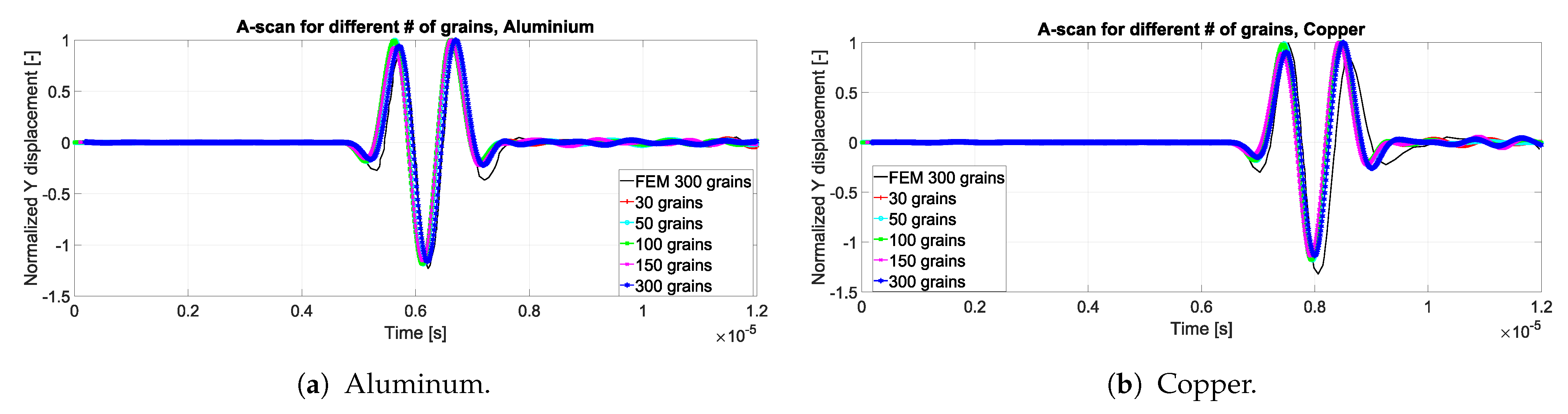
Figure 14 presents the comparison between the BEM and FEM solutions, in which both utilized 300 grains, for the Al and Cu materials. Since the wave velocity is influenced by the material properties, it was observed that the BEM model accurately captured this variation. Specifically, the Time of Arrival (ToA) for Al was 25% smaller compared to Cu, thus reflecting the fact that the wave velocity in Al is 25% greater than in Cu. Furthermore, a parametric study was conducted in the BEM simulation, whereby different numbers of grains were considered as ranging from 30 to 300. Figure 15 showcases the A-scan (back wall) signal received by the receiver probe for Al (Figure 15a) and Cu (Figure 15b). The symbol # in the figures refers to the number of grains. The figures demonstrate a remarkable agreement and alignment in terms of signal amplitude and phase between the BEM and FEM models, thus confirming BEM’s consistency for both materials.

3.5. Missing Grains: Porosity

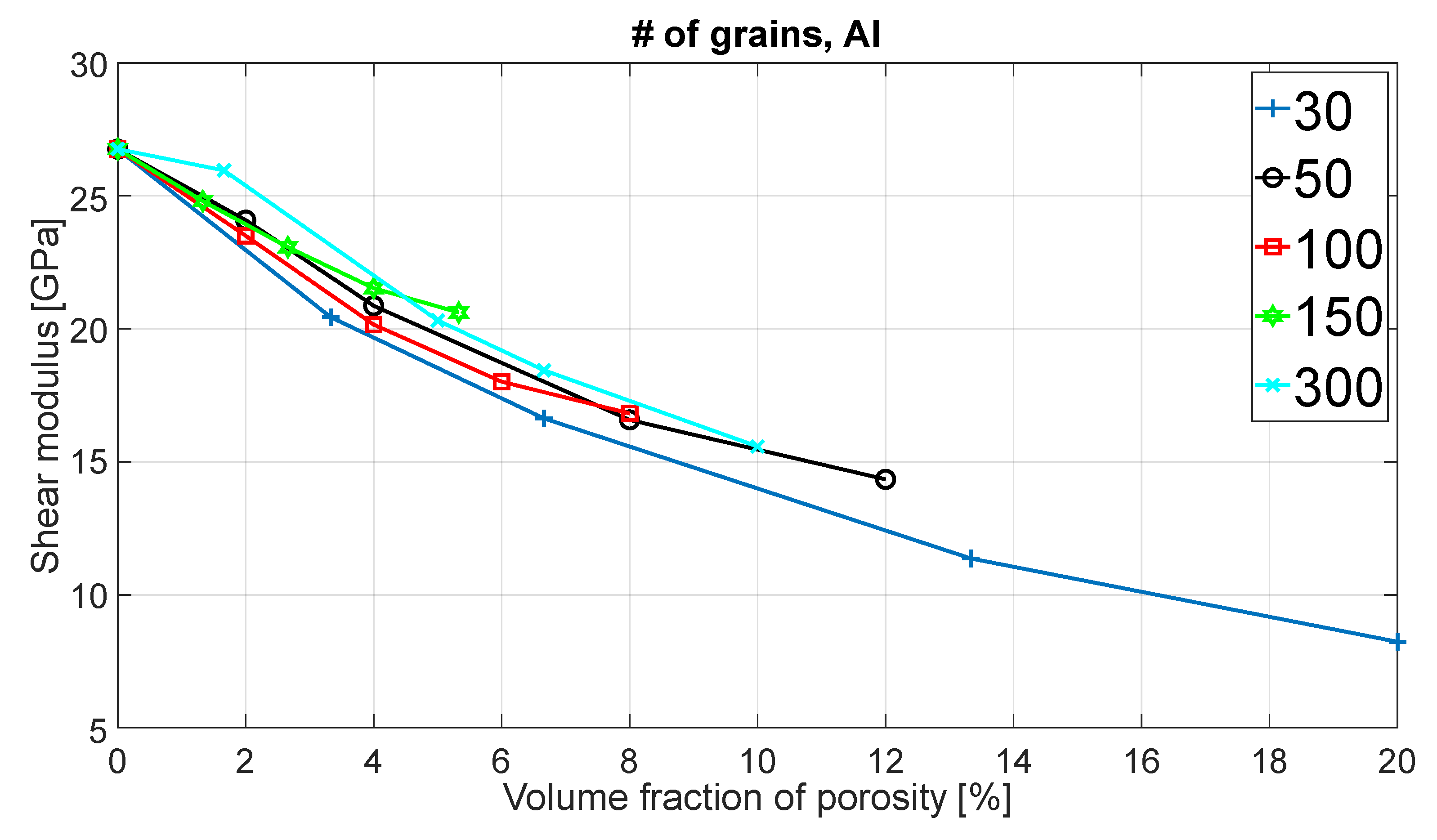
To investigate the impact of porosity on the macroscopic material properties, a parametric analysis was conducted by varying the number (#) of grains and the volume fraction of porosity [47,48,49]. The analysis was performed under the assumption of a plain strain condition, and the material considered was aluminum. The dimensions of the micro-structure were 100 × 100 [mm${}^2$]. The specific details of the porosity model employed in this study can be found in the corresponding section of this paper. To assess the macroscopic properties, such as the elastic modulus (E) and shear modulus (G), the homogenization approach based on the RVE was utilized. The procedure for evaluating these properties is explained in detail in the dedicated section of this paper.

The volume fraction of porosity was calculated with Equation (19). Figure 16 and Figure 17 show the Young and Shear moduli, respectively, against the volume fraction of porosity, thus sweeping the number of grains from 30 up to 300. As expected, the higher the volume fraction of porosity, the lower the Young and Shear moduli.

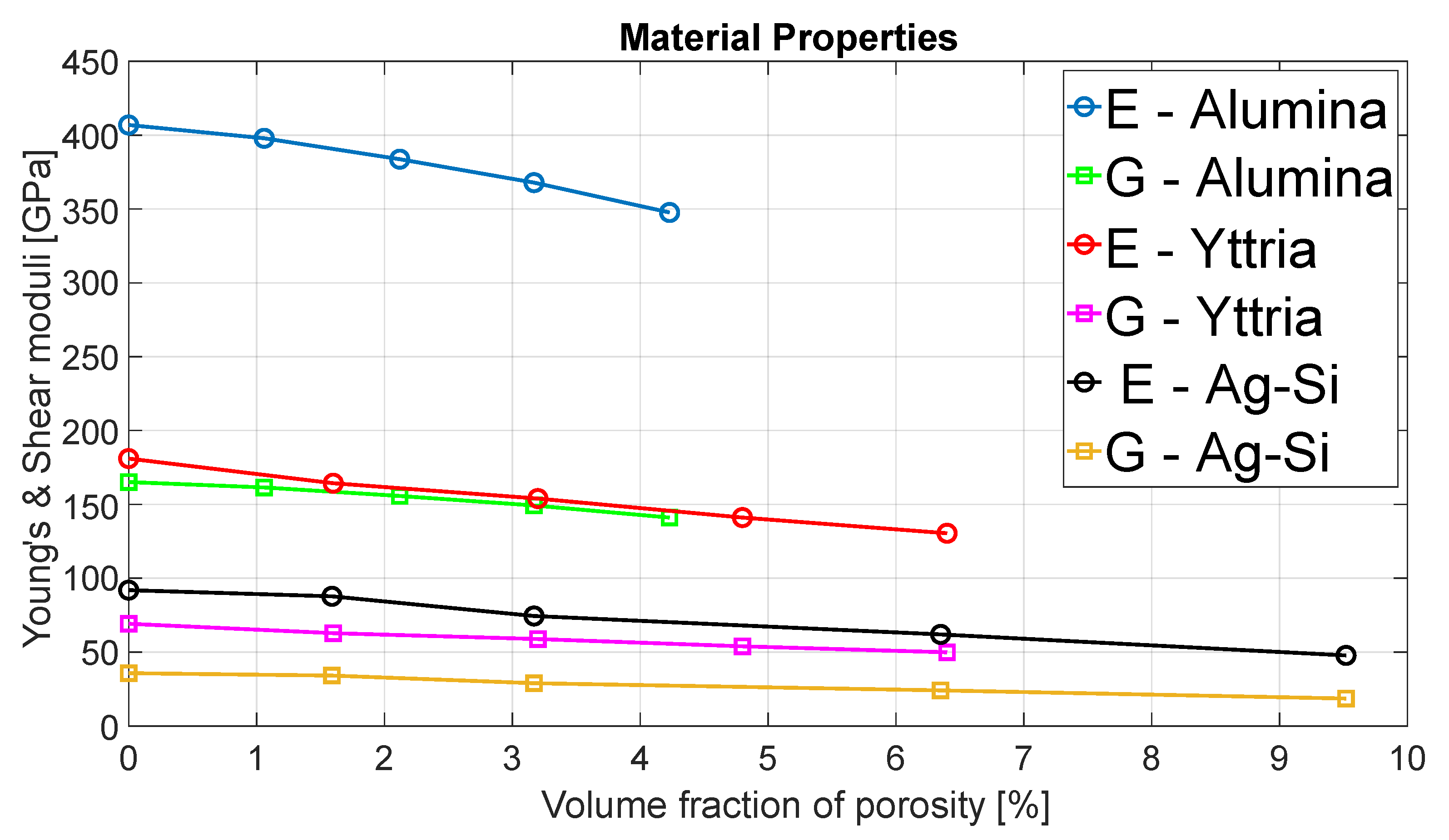
To investigate the impact of porosity on grain morphology, three different materials with distinct grain shapes were tested: gold-silver (Ag-Si) with a rhombic crystal morphology, yttria (Y₂O₃) with a cubic crystal morphology, and alumina (Al₂O₃) with a truncated octahedral crystal morphology. The material properties for each of these materials are provided in

Table 1. Material properties.

Material	Density $\left[\frac{\mathbf{kg}}{{\mathbf{m}}^3}\right]$	Young’s Modulus [GPa]	Poisson’s Ration
Gold−Silver (Ag-Si)	12,000–15,000	90	0.286
Yttria (Y2O3)	5010	174	0.308
Alumina (Al2O3)	3600	403	0.232

. Figure 18 illustrates the variation of both the Young and Shear moduli against the volume fraction of porosity for alumina (189 grains), yttria (125 grains), and Ag-Si (63 grains). As expected, an increase in the volume fraction of porosity lead to a decrease in both the Young and Shear moduli for all three materials.

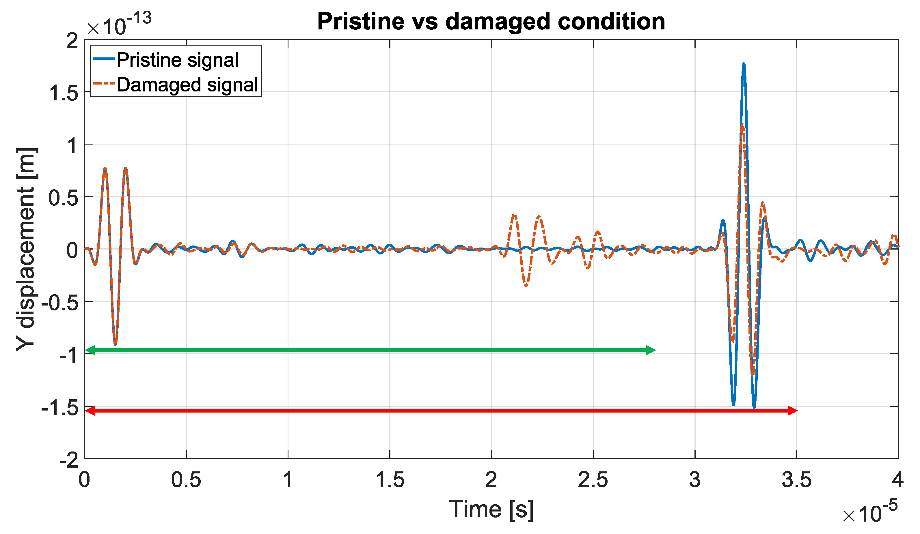
Furthermore, by analyzing the BEM results, it was possible to quantitatively evaluate the influence of the volume fraction of porosity on the macroscopic material properties.

Table 2. Material properties: Ag-Si.

${\mathit{V}}_{\mathit{f}}$ [%]	E [GPa]	G [GPa]	Diff E [%]	Diff G [%]
0	90	35	-	-
1.59	87.77	34.13	2.48	0.97
3.17	74.45	28.95	17.28	6.73
6.35	61.98	24.1	31.14	12.12
9.52	47.77	18.57	46.92	18.25

,

Table 3. Material properties: yttria.

${\mathit{V}}_{\mathit{f}}$ [%]	E [GPa]	G [GPa]	Diff E [%]	Diff G [%]
0	174	66.5	-	-
1.6	164.34	62.82	5.55	2.11
3.2	153.96	58.85	11.52	4.4
4.8	141.1	53.93	18.91	7.22
6.4	130.46	49.87	25.02	9.56

and

Table 4. Material properties: alumina.

${\mathit{V}}_{\mathit{f}}$ [%]	E [GPa]	G [GPa]	Diff E [%]	Diff G [%]
0	403	163.5	-	-
1.06	397.85	161.47	1.28	0.51
2.12	383.7	155.72	4.79	1.93
3.17	367.83	149.28	8.73	3.53
4.23	347.63	141.09	13.74	5.56

present the volume fraction of porosity, Young’s modulus, Shear modulus, and the percentage difference of E and G compared to the pristine condition for all three materials. The analysis revealed that the volume fraction of porosity had a greater effect on E compared to G, particularly for the rhombic crystal morphology (Ag-Si), while the effect was less pronounced for both the cubic crystal morphology (yttria) and the truncated octahedral crystal morphology (alumina). To conclude the porosity analysis, simulations were performed to detect the presence of voids. The detection of voids was analyzed based on the changes in the amplitude and ToA of the backscattered signal. The simulations were performed with voids in different positions for an aluminum micro-structure. The input signal was defined at the upper edge of the micro-structure, where a prescribed traction 3-cycle tone burst with a Hanning window and center frequency of 1 [MHz] was enforced. The time interval of the simulation was 40 [$\mathsf{\mu }$s] with a time step of 10 [ns] and a time interval of the excitation of 3 [$\mathsf{\mu }$s]. The ToA was calculated from 0 to the starting point of the wave packet backscattered by the void itself. The starting point of the wave packet backscattered by the void itself was evaluated as the value of the wave above a threshold.

Figure 19 illustrates the comparison between the averaged Y displacement at the upper edge for the pristine and the damaged conditions for a 50-grain micro-structure. The damaged signal (depicted by the orange line in the figure) clearly exhibited the presence of a void, as indicated by the amplitude of a signal that was backscattered by the void itself (the dashed green circle indicates the part of the wave that was located in the wave that was backscattered by the void itself). Thus, the BEM model successfully detected the presence of the void.

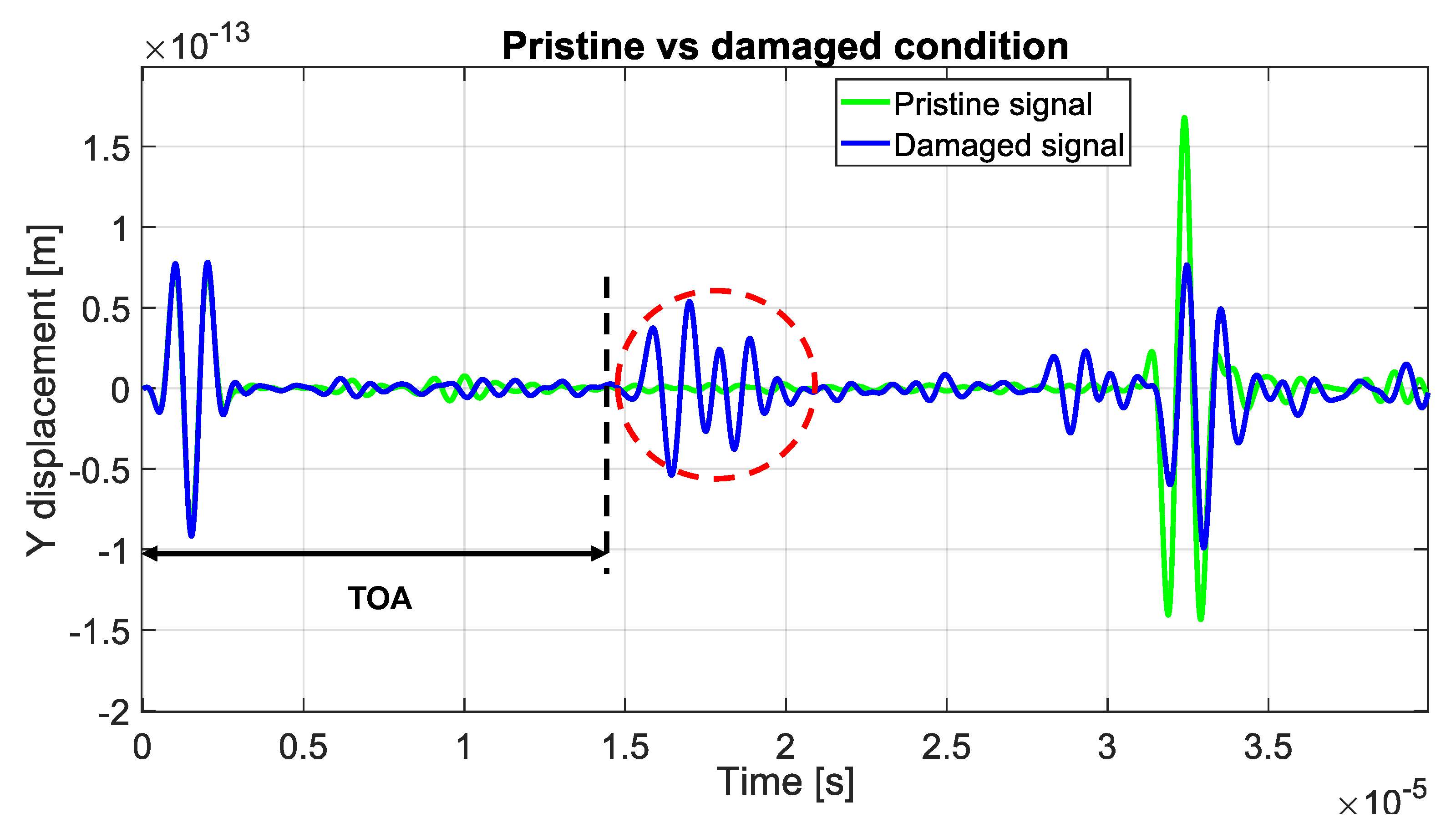
Similarly, Figure 20 presents the comparison between the averaged Y displacement at the upper edge for both the pristine and damaged conditions in 100-grain micro-structures. The damaged signal (represented by the blue line in the figure) revealed the presence of the void, which was confirmed by the amplitude of the signal that was backscattered by the void itself (the dashed red circle indicates the part of the wave that was located in the wave that was backscattered by the void itself). This demonstrated that the BEM model was capable of detecting the presence of voids that were located at different positions within the micro-structure.

3.6. Parametric Analysis with Inter-Granular Cracks (Debonding)

The presence of inter-granular cracks is a prevalent phenomenon in poly-crystalline materials because they can lead to debonding and subsequent material embrittlement, thus increasing the chance of significant risks such as structural failure [50,51,52,53,54]. Therefore, it is crucial to develop models that can accurately capture these failure mechanisms and the interaction with UGWs. To address this, a parametric analysis involving inter-granular cracks was conducted. In this analysis, aluminum micro-structures with dimensions of $100\times 100$ [mm${}^2$] were employed. Simulations were carried out by introducing cracks into the micro-structure while considering the following effects:

• Position/orientation: the cracks were located at the same distance from the upper edge with equal length but were positioned at different locations (left, center, and right);
• Crack length: the cracks were situated at the same distance from the upper edge, but varied in length;
• Distance: the cracks had the same length but were positioned at different distances from the upper edge.

Figure 21, Figure 22 and Figure 23 present illustrative examples for each effect, thus visually demonstrating the configurations of the cracks within the micro-structure.

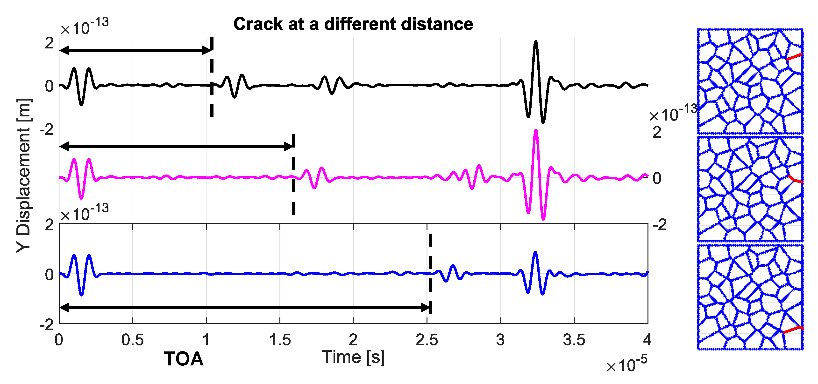
The excitation signal was applied at the upper edge of the structure, in which a prescribed traction with a 3-cycle tone burst with a Hanning window and center frequency of 1 [MHz] was utilized. The simulation duration was 40 [$\mathsf{\mu }$s], with a time step of 10 [ns] and an excitation time interval of 3 [$\mathsf{\mu }$s]. The ToA was calculated from the beginning of the simulation until the starting point of the wave packet, which was scattered by the crack itself for all three analyzed effects. The starting point of the wave packet that was scattered by the crack itself was evaluated as the value of the wave amplitude above a threshold. The simulated response corresponded to the averaged displacement over the entire upper edge against time. Figure 21 investigates the effect of the crack position and orientation. The cracks were randomly distributed in the simulated domain, and it could be observed that the numerical model successfully detected the presence of cracks based on the amplitude and ToA of the signal scattered by the cracks. Figure 22 evaluates the influence of the crack distance from the upper edge. As expected, it was observed that the ToA of the backscattered signal from the crack increased as the crack became more distant from the upper edge.

In Figure 23, the impact of crack length is examined. The signal amplitude that originated from the shortest crack (represented by the black signal) was comparable to the previously analyzed cases. However, as the crack length increased, the signal amplitude from the crack also increased. Consequently, the amplitude of the back-wall signal from the upper edge decreased for the green and purple signals, while the crack signal amplitude became more prominent. This illustrated that longer cracks have a greater influence on the overall signal amplitude. A summary of these findings can be found in

Table 5. Crack and back-wall signal amplitudes.

Signal	Crack Signal Amplitude [m]	Back-Wall Signal Amplitude [m]
Black color	$4.723\times$ 10${}^{-14}$	$1.201\times$ 10${}^{-13}$
Green color	$7.587\times$ 10${}^{-14}$	$1.073\times$ 10${}^{-14}$
Purple color	$1.377\times$ 10${}^{-13}$	$3.882\times$ 10${}^{-15}$

.

3.7. Probability of Detection (PoD) with Inter-Granular Cracks

The Probability of Detection (PoD) curve method was extensively employed for evaluating the reliability of NDT techniques. The PoD represents the capability of an NDT method to detect a flaw of specific characteristics, such as type and size. PoD curves are constructed based on the characteristic dimensions of a certain defect, such as depth, length, orientation. These curves are influenced by various factors, including material properties, geometric features, defect types, operator skills, and environmental conditions [55,56]. Generating PoD curves typically requires a significant amount of experimental data, which can be expensive and time-consuming [57,58]. Consequently, there has been growing interest in utilizing simulation methods to reduce the reliance on extensive experimental testing. The concept of Model-Assisted and/or Simulation-Supported PoD has emerged in the past two decades, in which the aim is to leverage analytical or numerical models to enhance the efficiency and accuracy of PoD curve determination [59,60,61]. Building upon the framework of Model-Assisted Probability of Detection (MAPoD), which has been utilized in numerous studies exploring simulation-based approaches to replace or supplement model-based approaches [60,61,62], this research endeavors to investigate the feasibility of employing BEM simulations for generating PoD curves in the ultrasonic inspection of poly-crystalline micro-structures. To incorporate the influence of variability factors into the simulation, as well as to subsequently calculate the MAPoD, it is necessary to consider the potential sources of variability. For simplicity in this study, the sources of variability considered were the number of grains and grain morphologies, the material property variations, as well as crack length, crack orientation, and crack position. Specifically, the number of grains considered were 30, 50, and 100. For each number of grains, five different grains morphologies were considered, where the Young’s modulus varied within a range of 5% around the mean value for the corresponding material. The material under investigation was aluminum. The crack length was varied from $0.5$ to 7 [mm], in increments of $0.5$ [mm]. Both the location and orientation of the cracks were randomly distributed. Thus, 10 cracks located and orientated randomly for each crack length and for each grain morphology were considered, thereby resulting in a total of 50 combinations of variability sources per crack length. Consequently, a total of 700 simulations were conducted. Upon completion of all the simulations, the resulting scatter plot of the flaw responses was utilized to construct the PoD curve. The averaged vertical displacement at the upper edge was selected as the output signal. Snapshots from the BEM simulations that considered different scenarios are presented in Figure 24, Figure 25, Figure 26, Figure 27 and Figure 28.

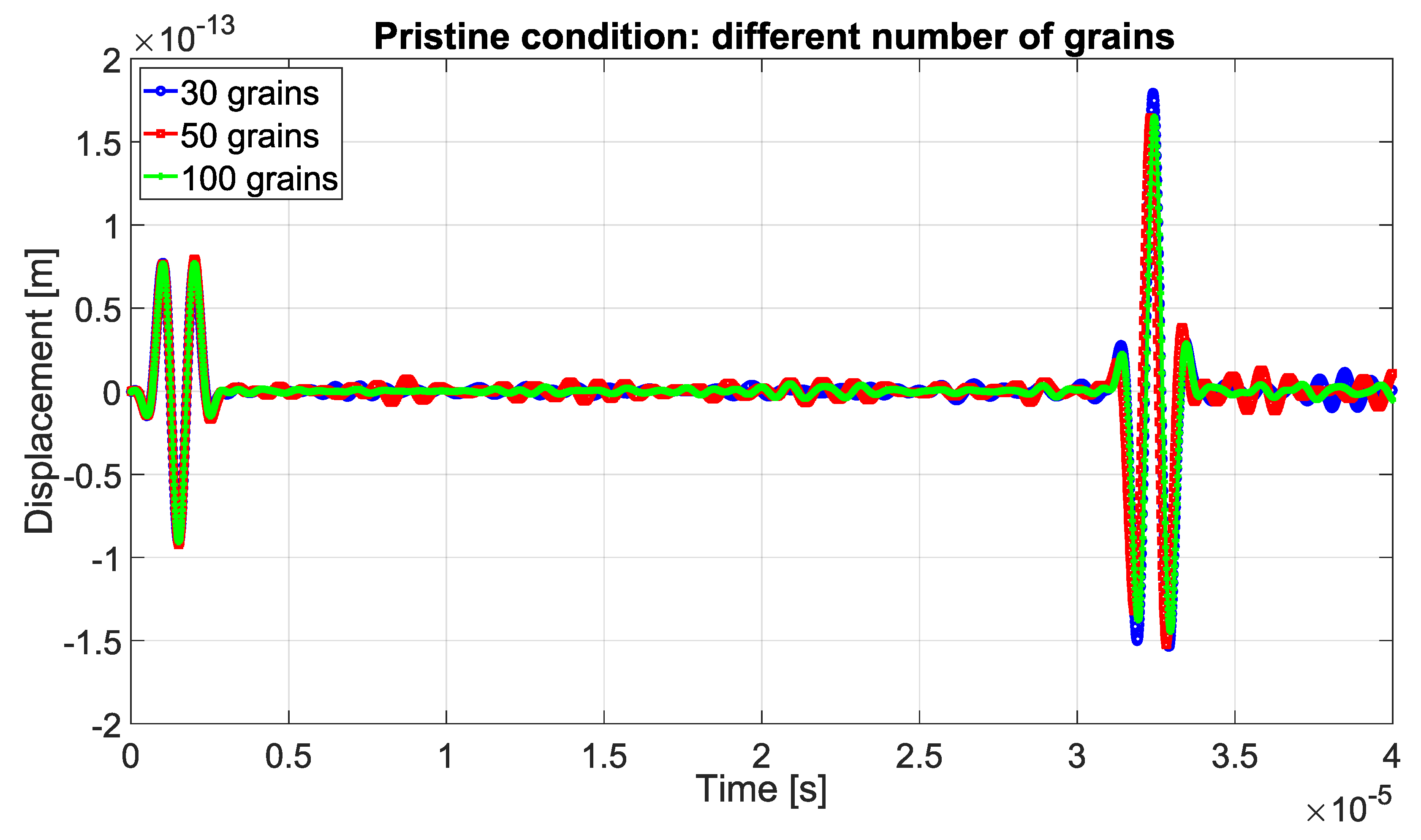
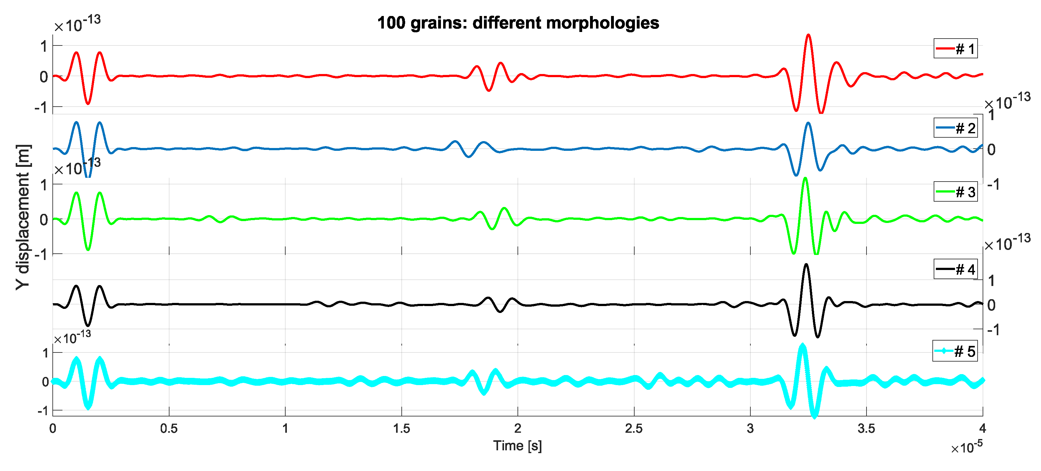
Figure 24 illustrates the averaged pristine signal obtained at the upper edge of the structure for varying numbers of grains, specifically 30, 50, and 100. As depicted in the figure, the signals exhibited excellent agreement in terms of both amplitude and the ToA. Figure 25 showcases a comparison of the signals generated from different grain morphologies while maintaining a fixed number of grains (i.e., 100 grains in this particular case). Notably, these five signals exhibited slight variations, particularly in terms of the ToA, because of the presence of distinct grain morphologies and their associated material properties.

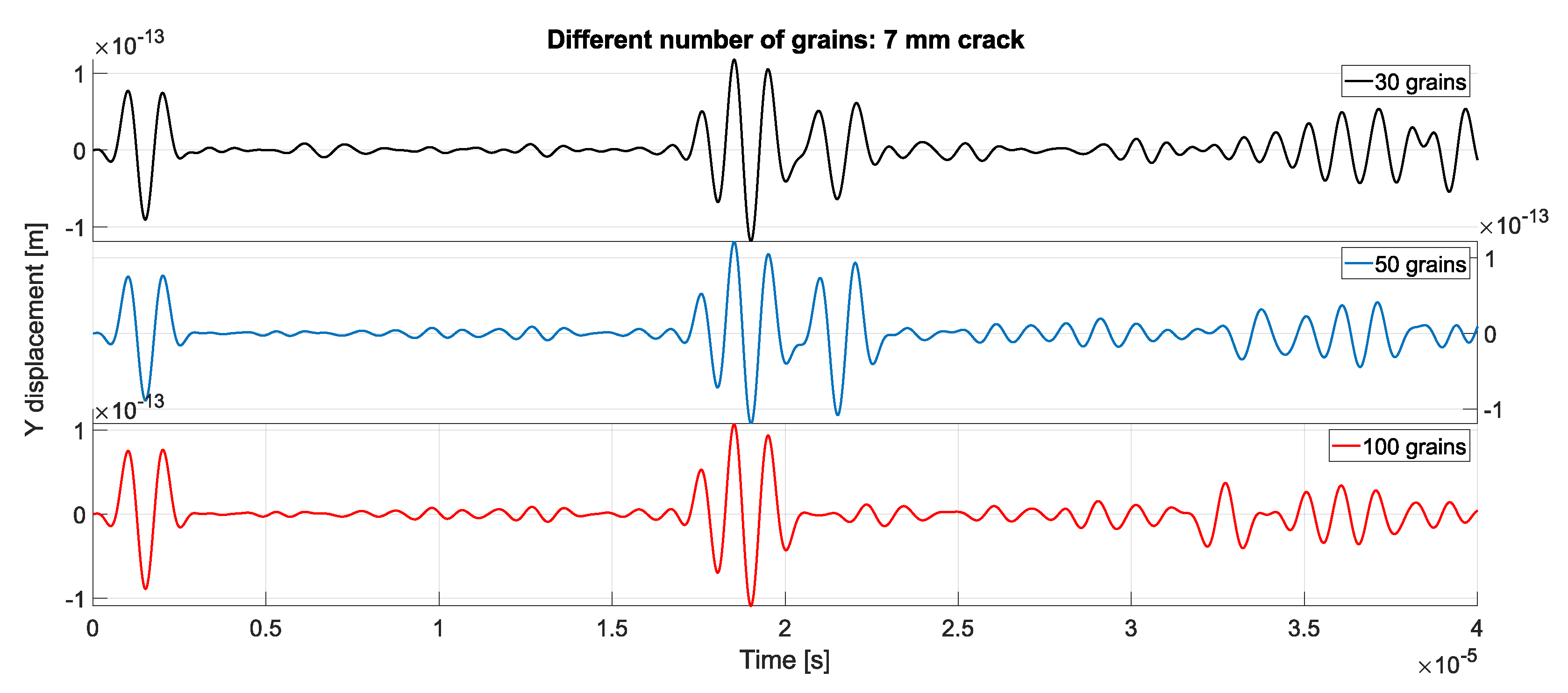
Figure 26 presents the signals obtained under the damaged condition, specifically with a 7 [mm] crack, for varying numbers of grains. As observed in the figure, there was a noticeable increase in the signal amplitude that originated from the crack as the crack length increased. Consequently, the amplitude of the backscattered signal from the upper edge decreased, thereby indicating that long cracks significantly impact the overall signal amplitude.

Figure 27 presents the signals obtained under the damaged condition with varying crack orientations, namely $0^{\circ }$, ${30}^{\circ }$, and ${45}^{\circ }$. Notably, the backscattered signal from the crack with a $0^{\circ }$ orientation exhibited the highest amplitude, while the amplitude decreased as the crack angle increased. This behavior can be attributed to the fact that the wave is perpendicular to the $0^{\circ }$ crack, thus resulting in maximum signal strength. Furthermore, the duration of the backscattered signal increased with an increasing crack angle. This is because of the decrease in signal amplitude, which requires more time for the same energy to be dissipated.

Figure 28 displays the signals obtained for a 2 [mm] crack length, in which different numbers of grains were considered. As depicted in the figure, the signals exhibited excellent agreement in both amplitude and the ToA.

To eliminate the effect of multiple boundaries reflecting the signal, there were two choices to select with respect to the inspection interval (time window):

• Up to the first back-wall reflection signal (time interval in red arrows in Figure 29);
• Up to the damaged backscattered signal (time interval in green arrows in Figure 29).

In this study, the selected time interval of inspection was the first one and, in the case that the first wave packet was ambiguous and could not be clearly identified, the time window for the first wave packet was manually determined based on the signal characteristics.

Let $D_i$ denote the damaged signal and let $P_i$ denote the corresponding pristine state signal. The residual signal $r_i$, was obtained by subtracting the pristine signal from its damaged signal: $r_i=D_i-P_i$. Many existing approaches for damage detection involve extracting damage-sensitive features from UGW signals and establishing an index that indicates the presence of damage (commonly referred to as the Damage Index (DI)). The damage index was then compared to a threshold value, above which the presence of damage was signified. The damage detection strategy involved comparing the current signal with its baseline signal and quantifying the changes. In this case, the current signals were recorded under the same environmental and loading conditions, and any deviation from the baseline signal was attributed to the presence of damage. The magnitude of the deviation was quantified by the DI. The damage index used in this analysis was the reduction in correlation coefficient between the signal and its baseline, noted as ${DI}_{SDC}$:

$${DI}_{SDC}=SDC=1-\left|\frac{Cov\left(P_i,D_i\right)}{{\sigma }_{P_i},{\sigma }_{D_i}}\right|=1-\frac{{\sum }_{t=0}^T\left(D_i-{\sigma }_{D_i}\right)\left(P_i-{\sigma }_{P_i}\right)}{{\sigma }_{P_i},{\sigma }_{D_i}},$$

(20)

where $Cov\left(P_i,D_i\right)$ is the covariance of the signals and ${\sigma }_{I_j}$ is the standard deviation of the signals, respectively. This damage index takes into consideration both the difference in amplitude and in the ToA.

There are many ways to evaluate the threshold value. In this study, the threshold value was evaluated as follows:

• Fixing the morphology;
• Changing the frequency with a mean of 1 [MHz] and standard deviation of $5\%$ (uncertainty on frequency);
• Changing the location of the actuation signal (uncertainty on location).

The DI in the pristine state was evaluated with the following:

$${DI}_{pristine}=1-\left|\frac{Cov\left(P_i,P_j\right)}{{\sigma }_{P_i},{\sigma }_{P_j}}\right|=1-\frac{{\sum }_{t=0}^T\left(P_j-{\sigma }_{P_j}\right)\left(P_i-{\sigma }_{P_i}\right)}{{\sigma }_{P_i},{\sigma }_{P_j}}$$

(21)

where $P_i$ is the signal in a pristine state with a fixed actuation signal location and 1 [MHz] frequency, while $P_j$ is the signal in a pristine state with uncertainties in both the actuation location and the frequency. As this procedure was followed for each morphology, five different DIs in pristine condition were obtained. Figure 30 shows the DI in a pristine condition for the 100-grain case with a fixed morphology (i.e., $\#1$). The DI exhibited a normal distribution, as illustrated by the black line on the right side of the plot. The dashed red lines refer to one standard deviation or $1\sigma$. The DI values ranged from 0.24 to 0.34, with a mean value of 0.29.

Figure 31 presents the DI in a damaged condition for the 100-grain case (morphology $\#1$), which was plotted against the crack length. As expected, the results clearly demonstrated that the DI increased with an increase in crack length. The dashed red line corresponds to the threshold value, while the dashed black line represents the mean value of the DI for each crack length.

There were two main approaches commonly employed to generate PoD curves, namely, hit/miss data and signal response analysis (“$\widehat{a}$” vs. “a”) [60,61]. The hit/miss approach provided binary results, indicating whether a flaw of a known size was detected or not. In this analysis, the number of detected cracks, “n”, was divided by the total number of simulated cracks, “N”, thereby yielding a reasonable assessment of the inspection system’s capability, $PoD=\frac{n}{N}$. This approach provided a single value representing the entire range of crack sizes. However, since larger cracks are typically easier to detect than smaller ones, cracks are often grouped based on their sizes, and $\frac{n}{N}$ was calculated for each size range. Figure 32 illustrates the PoD obtained using the hit/miss approach, which was plotted against the crack length. As depicted in the figure, the PoD increased as the crack length increased, reaching its maximum at a crack length of 5 [mm].

The second approach for determining the PoD was of much interest for several practical applications since it gave more information through the recorded defect response “$\widehat{a}$”, which was correlated with the defect characteristic dimension “a” [60,61,63,64]. This method utilizes regression analysis with Maximum Likelihood Estimation (MLE) to calculate the regression coefficients and their covariance matrix. From the variance of the expected regression response, confidence bounds at a $95\%$ level can be constructed for “a”. To compute the PoD parameters, the threshold value was determined based on the consideration stated before. The variance ($var\left(PoD\right)$) was utilized to estimate confidence intervals and the covariance matrix for PoD. The PoD could be generated for each crack by calculating the probability of the signal response when it exceeds the decision threshold value. In this analysis, the target variable was the crack length. Figure 33 depicts the regression analysis for the 100-grain case, where the crack length is represented on the “x” axis and the DI is displayed on the “y” axis.

Figure 34 illustrates the PoD curve for the 100-grain case as a function of crack length. The important features of the model were recorded on the curve, including the $95\%$ confidence interval (CI) area, as well as both the lower and upper bound of the PoD curve and the mean value. Furthermore, the $a_{\frac{90}{95}}$ value, which is the $95\%$ confidence bound on the $a_{90}$ estimate, is displayed in the plot.

As depicted in Figure 34, the PoD exhibits the expected behavior, where an increase in crack length corresponds to an increase in PoD. The PoD curves obtained from the BE simulations aligned with this expectation, thus demonstrating the potential of simulations for PoD characterization (particularly for crack lengths exceeding 3 [mm]). However, within the defect length range of 0–3 [mm], the PoD values were notably low. This discrepancy may be attributed to the limitations of the assumed parameters in the BEM simulations, which failed to accurately capture the intricacies associated with the smaller cracks in reality. Additionally, factors such as the noise sources that diminished the measured reflection amplitude, as well as the actual conditions of the wave generation and reception, needed to be incorporated into the simulations for a more comprehensive representation. Ongoing research aims to refine the representation and establish bounds for parameter uncertainties, which will contribute to enhanced predictions of PoD based on the BEM approach.

However, for defect lengths ranging from 0 to 3 [mm], a low PoD value was observed, possibly due to uncertainties in the assumed parameters not capturing the reality for smaller cracks. Incorporating finer details such as noise sources, which reduce the amplitude of measured reflection, and realistic wave generation and reception conditions into simulations is an ongoing effort to improve the accuracy of PoD predictions based on the BEM.

4. Conclusions

In this paper, a numerical method based on the BEM was developed for the SHM of poly-crystalline micro-structures at micro-scale. The proposed method wasused to investigate how the micro-structural features affect the macro-structural properties of poly-crystalline materials, as well as to understand the resulting changes in both wave propagation and wave-material interaction. In investigating the influence of micro-structural features on both macro-structural properties and wave–material interactions, the novel contribution of this work lies in the integration of BEM and UGWs as numerical tools for the SHM characterization of poly-crystalline materials. The method was validated through experimental tests, thereby demonstrating an agreement between numerical and experimental results. The validation confirmed the reliability of the physical measurements and the effectiveness of the numerical simulation in capturing the behavior and characteristics of the investigated system. Through exploring pristine and damaged conditions, the study analyzed the impact of porosity and inter-granular cracks on the overall structural response. The phenomenon called porosity was quantitatively and qualitatively investigated. The influence of the volume fraction of porosity on material macro-properties was analyzed. An increase in the volume fraction of porosity lead to a decrease in the material macro-properties. Furthermore, the detection of voids was considered based on the amplitude and the ToA of the signal that was backscattered by the void itself. This study also investigated inter-granular cracks, which can lead to embrittlement and laceration. Parametric analyses were conducted to examine the effects of crack position/orientation, crack length, and crack distance from a specific reference. The presence of cracks was detected by the BEM model, and longer cracks resulted in a larger amplitude of the backscattered signal. Additionally, the ToA increased with the distance of the crack from the reference point. As a result of these analyses, the BEM method provided insights into wave propagation and wave–material interactions at the micro-scale, for both voids and inter-granular cracks. A framework is proposed for generating Probability of Detection (PoD) curves based on two models using numerical simulations. The PoD curves demonstrated an increase in the Probability of Detection with increasing crack length, thus showing promise for cracks longer than 3 [mm]. Ongoing research aims to refine representation and address the parameter uncertainties for improved PoD predictions within the 0 to 3 [mm] defect length range, where a low PoD value was observed. This study concluded that the BEM and UGW numerical simulations offer efficient and reliable approaches for understanding micro-structural features and the wave–material interactions within poly-crystals at micro-scale. Even though each grain has its own material properties, orientation, and crystal orientation, the model assumes isotropic behavior. Hence, future research will implement anisotropic or orthotropic material models for more accurate micro-structure representations.

References

- Shivaprasad, S.; Pandala, A.; Krishnamurthy, C.; Balasubramaniam, K. Wave localized finite-difference-time-domain modelling of scattering of elastic waves within a polycrystalline material. J. Acoust. Soc. Am. 2018, 144, 3313–3326. [Google Scholar] [CrossRef] [PubMed]
- Geraci, G. Boundary Element Methods for Cohesive Thermo-Mechanical Damage and Micro-Cracking Evolution. Ph.D. Thesis, Imperial College London, London, UK, 2018. [Google Scholar]
- Raghavan, A. Guided-Wave Structural Health Monitoring. Ph.D. Thesis, University of Michigan, Ann Arbor, MI, USA, 2007. [Google Scholar]
- Sause, M.G.R.; Jasiuniene, E. Structural Health Monitoring Damage Detection Systems for Aerospace, 1st ed.; Springer Open: Berlin/Heidelberg, Germany, 2021; pp. 1–284. [Google Scholar]
- Ding, Y.; Ye, X.W.; Guo, Y. Data set from wind, temperature, humidity and cable acceleration monitoring of the Jiashao bridge. J. Civ. Struct. Health Monit. 2023, 13, 579–589. [Google Scholar] [CrossRef]
- Yuan, F.-G. Structural Health Monitoring (SHM) in Aerospace Structures, 1st ed.; Elsevier: Amsterdam, The Netherlands, 2016; pp. 1–514. [Google Scholar]
- Ding, Y.; Ye, X.-W.; Guo, Y. A Multistep Direct and Indirect Strategy for Predicting Wind Direction Based on the EMD-LSTM Model. Struct. Control Health Monit. 2023, 1, 1–13. [Google Scholar] [CrossRef]
- Rose, J.L. Ultrasonic Guided Waves in Solid Media, 1st ed.; Cambridge University Press: Cambridge, UK, 2014; pp. 1–507. [Google Scholar]
- Zou, F. A Boundary Element Method for Modelling Piezoelectric Transducer Based Structural Health Monitoring. Ph.D. Thesis, Imperial College London, London, UK, 2015. [Google Scholar]
- Aghaie-Khafri, M.; Honarvar, F.; Zanganeh, S. Characterization of grain size and yield strength in aisi 301 stainless steel using ultrasonic attenuation measurements. J. Nondestruct. Eval. 2012, 31, 191–196. [Google Scholar] [CrossRef]
- Grabec, M.; Sedlák, T.P.; Veres, I.A. Influence of grain morphology on ultrasonic wave attenuation in polycrystalline media with statistically equiaxed grains. J. Acoust. Soc. Am. 2018, 143, 219–229. [Google Scholar]
- Arguelles, A.P.; Turner, J.A. Ultrasonic attenuation of polycrystalline materials with a distribution of grain sizes. J. Acoust. Soc. Am. 2017, 141, 4347–4353. [Google Scholar] [CrossRef]
- Geraci, G.; Aliabadi, M. Micromechanical boundary element modelling of transgranular and intergranular cohesive cracking in polycrystalline materials. Eng. Fract. Mech. 2017, 176, 351–374. [Google Scholar] [CrossRef]
- Sfantos, G.; Aliabadi, M. A boundary cohesive grain element formulation for modelling intergranular microfracture in polycrystalline brittle materials. Int. J. Numer. Methods Eng. 2007, 69, 1590–1626. [Google Scholar] [CrossRef]
- Benedetti, I.; Barbe, F. Modelling Polycrystalline Materials: An Overview of Three-Dimensional Grain-Scale Mechanical Models. J. Multiscale Model. 2013, 5, 1–51. [Google Scholar] [CrossRef]
- Van Pamel, A.; Sha, G.; Rokhlin, S.I.; Lowe, M.J. Finite-element modelling of elastic wave propagation and scattering within heterogeneous media. Proc. R. Soc. A Math. Phys. Eng. Sci. 2017, 473, 20160738. [Google Scholar] [CrossRef]
- Van Pamel, A.; Brett, C.R.; Huthwaite, P.; Lowe, M.J. Finite element modelling of elastic wave scattering within a polycrystalline material in two and three dimensions. J. Acoust. Soc. Am. 2015, 138, 2326–2336. [Google Scholar] [CrossRef]
- Levander, A.R. Fourth-order finite-difference P-SV seismograms. Geophysics 1988, 53, 1425–1436. [Google Scholar] [CrossRef]
- Souza, L.A.; Carrer, J.A.M.; Martins, C.J. A fourth order finite difference method applied to elastodynamics: Finite element and boundary element formulations. Struct. Eng. Mech. 2004, 17, 735–749. [Google Scholar] [CrossRef]
- Shivaprasad, S.; Krishnamurthy, C.; Pandala, A.; Saini, A.; Ramachandran, A.; Balasubramaniam, K. Numerical Modelling Methods for Ultrasonic Wave Propagation Through Polycrystalline Materials. Trans. Indian Inst. Met. 2019, 72, 2923–2932. [Google Scholar] [CrossRef]
- Fellinger, P.; Marklein, R.; Langenberg, K.J.; Klaholz, S. Numerical modeling of elastic wave propagation and scattering with EFIT—Elastodynamic finite integration technique. Wave Motion 1995, 21, 47–66. [Google Scholar] [CrossRef]
- Song, C.; Wolf, J.P. The scaled boundary finite-element method—Alias consistent infinitesimal finite-element cell method—For elastodynamics. Comput. Methods Appl. Mech. Eng. 1997, 147, 329–355. [Google Scholar] [CrossRef]
- Gravenkamp, H. Numerical Methods for the Simulation of Ultrasonic Guided Waves. Ph.D. Thesis, TU Braunschweig, Braunschweig, Germany, 2014. [Google Scholar]
- Sha, G. Analytical attenuation and scattering models for polycrystals with uniform equiaxed grains. J. Acoust. Soc. Am. 2018, 143, EL347–EL353. [Google Scholar] [CrossRef]
- Ghoshal, G.; Turner, J.A. Numerical model of longitudinal wave scattering in polycrystals. IEEE Trans. Ultrason. Ferroelectr. Freq. Control 2009, 56, 1419–1428. [Google Scholar] [CrossRef]
- Dupond, O.; Feuilly, N.; Chassignole, B.; Fouquet, T.; Moysan, J.; Corneloup, G. Relation between ultrasonic backscattering and microstructure for polycrystalline materials. J. Phys. Conf. Ser. 2011, 269, 1–8. [Google Scholar] [CrossRef]
- Liu, Y.; Van Pamel, A.; Nagy, P.B.; Cawley, P. Investigation of ultrasonic backscatter using three-dimensional finite element simulations. J. Acoust. Soc. Am. 2019, 145, 1584–1595. [Google Scholar] [CrossRef]
- Pandala, A.; Shivaprasad, S.; Krishnamurthy, C.; Balasubramaniam, K. Modelling of Elastic Wave Scattering in Polycrystalline Materials. In Proceedings of the 8th International Symposium on NDT in Aerospace, Bangalore, India, 3–5 November 2016; Volume 22, pp. 1–9. [Google Scholar]
- Li, J. Boundary Element Plate Formulations for Dynamic Fracture and Ultrasonic Guided-Wave Structural Health Monitoring. Ph.D. Thesis, Imperial College London, London, UK, 2020. [Google Scholar]
- Aliabadi, M.H.F. The Boundary Element Method, Volume 2: Applications in Solids and Structures, 1st ed.; John Wiley & Sons: Chichester, UK, 2002; pp. 1–593. [Google Scholar]
- Liu, E.; Zhang, Z. Numerical Study pf Elastic Wave Scattering by Cracks or Inclusions Using the Boundary Integral Equation Method. J. Comput. Acoust. 2001, 9, 1039–1054. [Google Scholar] [CrossRef]
- Schafbuch, P.J.; Thompson, R.B.; Rizzo, F.J. Application of the boundary element method to elastic wave scattering by irregular defects. J. Nondestruct. Eval. 1990, 9, 113–127. [Google Scholar] [CrossRef]
- Fedelinski, P.; Aliabadi, M.; Rooke, D. The laplace transform DBEM for mixed-mode dynamic crack analysis. Comput. Struct. 1996, 59, 1021–1031. [Google Scholar] [CrossRef]
- Fedelinski, P.; Aliabadi, M.; Rooke, D. A single-region time domain BEM for dynamic crack problems. Int. J. Solids Struct. 1995, 32, 3555–3571. [Google Scholar] [CrossRef]
- Cruse, T.A.; Rizzo, F.J. A direct formulation and numerical solution of the general transient elastodynamic problem. I. J. Math. Anal. Appl. 1968, 22, 244–259. [Google Scholar] [CrossRef]
- Cruse, T.A. A direct formulation and numerical solution of the general transient elastodynamic problem. II. J. Math. Anal. Appl. 1968, 22, 341–355. [Google Scholar] [CrossRef]
- Vetterling, W.T.; Press, W.H.; Teukolsky, S.A.; Flannery, B.P. Numerical Recipes in Fortran, the Art of Scientific Computing, 1st ed.; Cambridge University Press: Cambridge, UK, 1994; pp. 1–973. [Google Scholar]
- Hearmon, R.F.S. Numerical Data and Functional Relationships in Science and Technology: Group III, Crystal and Solid State Physics, Vol. 1, Elastic, Piezoelectric Piezooptic and Electrooptic Constants of Crystals, 1st ed.; Hellwege, K.H., Ed.; Springer: Berlin/Heidelberg, Germany, 1966. [Google Scholar]
- American Society for Testing and Materials (ASTM). Standard test methods for determining average grain size, e112-13. ASTM Int. 2013, 1, 1–28. [Google Scholar]
- Schneider, C.A.; Rasband, W.S.; Eliceiri, K.W. Nih image to imagej: 25 years of image analysis. Nat. Methods 2012, 9, 671–675. [Google Scholar] [CrossRef]
- Van Pamel, A.; Nagy, P.B.; Lowe, M.J. On the dimensionality of elastic wave scattering within heterogeneous media. J. Acoust. Soc. Am. 2016, 140, 4360–4366. [Google Scholar] [CrossRef]
- Van Pamel, A.; Huthwaite, P.; Brett, C.R.; Lowe, M.J. Numerical simulations of ultrasonic array imaging of highly scattering materials. NDT E Int. 2016, 81, 9–19. [Google Scholar] [CrossRef]
- Van Pamel, A.; Huthwaite, P.; Brett, C.; Lowe, M. A finite element model investigation of ultrasonic array performance for inspecting polycrystalline materials. AIP Conf. Proc. Am. Inst. Phys. 2015, 1650, 1007–1014. [Google Scholar]
- Boström, A.; Ruda, A. Ultrasonic Attenuation in Polycrystalline Materials in 2D. J. Nondestruct. Eval. 2019, 38, 47. [Google Scholar] [CrossRef]
- Van Pamel, A.; Huthwaite, P.; Brett, C.R.; Lowe, M.J.S. Finite element modelling of wave propagation in highly scattering materials. AIP Conf. Proc. 2016, 1706, 070001. [Google Scholar]
- Shivaprasad, S.; Balasubramaniam, K.; Krishnamurthy, C.V. Voronoi based microstructure modelling for elastic wave propagation. AIP Conf. Proc. 2016, 1706, 070013. [Google Scholar]
- Asmani, M.; Kermel, C.; Leriche, A.; Ourak, M. Influence of porosity on young’s modulus and poisson’s ratio in alumina ceramics. J. Eur. Ceram. Soc. 2001, 21, 1081–1086. [Google Scholar] [CrossRef]
- Phani, K.K. Estimation of elastic properties of porous ceramic using ultrasonic longitudinal wave velocity only. J. Am. Ceram. Soc. 2007, 90, 2165–2171. [Google Scholar] [CrossRef]
- Chang, L.S.; Chuang, T.H. Characterization of alumina ceramics by ultrasonic testing. Mater. Charact. 2000, 45, 221–226. [Google Scholar] [CrossRef]
- Chen, H.L.R.; Zhang, B.; Alvin, M.A.; Lin, Y. Ultrasonic detection of delamination and material characterization of thermal barrier coatings. J. Therm. Spray Technol. 2012, 21, 1184–1194. [Google Scholar] [CrossRef]
- Eren, E.; Kurama, S.; Solodov, I. Characterization of porosity and defect imaging in ceramic tile using ultrasonic inspections. Ceram. Int. 2012, 38, 2145–2151. [Google Scholar] [CrossRef]
- Chen, B.; Li, W.; Qing, X. Damage detection of thermal barrier coating by ultrasonic guided wave. IOP Conf. Ser. Mater. Sci. Eng. 2019, 493, 1–9. [Google Scholar] [CrossRef]
- Chen, R.H.; Zhang, B.; Alvin, M.A. Ultrasonic detection of delamination and material characterization of thermal barrier coatings. Turbo Expo Power Land Sea Air 2009, 48852, 925–932. [Google Scholar] [CrossRef]
- Lin, L.; Zhao, Y.; Chen, J.; Li, X.; Lei, M. Ultrasonic characterization of eb-pvd thermal barrier coatings irradiated by hipib. Key Eng. Mater. 2008, 373, 358–362. [Google Scholar] [CrossRef]
- Ding, Y.; Ye, X.-W.; Guo, Y.; Zhang, R.; Ma, Z. Probabilistic method for wind speed prediction and statistics distribution inference based on SHM data-driven. Probab. Eng. Mech. 2023, 73, 1–9. [Google Scholar] [CrossRef]
- Ding, Y.; Ye, X.-W.; Guo, Y. Copula-based JPDF of wind speed, wind direction, wind angle, and temperature with SHM data. Probab. Eng. Mech. 2023, 73, 1–10. [Google Scholar] [CrossRef]
- Ding, Y.; Ye, X.-W.; Su, Y.-H.; Zheng, X.-L. A framework of cable wire failure mode deduction based on Bayesian network. Structures 2023, 57, 1–11. [Google Scholar] [CrossRef]
- Ding, Y.; Ye, X.-W.; Guo, Y. Wind load assessment with the JPDF of wind speed and direction based on SHM data. Structures 2023, 47, 2074–2080. [Google Scholar] [CrossRef]
- MAPOD. Available online: http://www.cnde.iastate.edu/mapod/ (accessed on 7 July 2022).
- Annis, C. MIL-HDBK-1823A, Nondestructive Evaluation System Reliability Assessment; Department of Defense Handbook, Wright-Patterson AFB: Greene County, OH, USA, 2009; Volume 1, pp. 1–171. [Google Scholar]
- Gandossi, L.; Annis, C. Probability of Detection Curves: Statistical Best-Practices; ENIQ Report No 41; EUR 24429 EN; European Commission Joint Research Centre Institute for Energy: Petten, The Netherlands, 2010; Volume 1, pp. 1–72. [Google Scholar]
- Subair, S.M.; Balasubramaniam, K.; Rajagopal, P.; Kumar, A.; Rao, B.P.; Jayakumar, T. Finite element simulations to predict probability of detection (pod) curves for ultrasonic inspection of nuclear components. Procedia Eng. 2014, 86, 461–468. [Google Scholar] [CrossRef]
- Ali, M.S.S.A.; Kumar, A.; Rao, P.B.; Tammana, J.; Balasubramaniam, K.; Rajagopal, P. Bayesian synthesis for simulation-based generation of probability of detection (pod) curves. Ultrasonics 2018, 84, 210–222. [Google Scholar]
- Subair, S.M.; Agrawal, S.; Balasubramaniam, K.; Rajagopal, P.; Kumar, A.; Rao, P.B.; Tamanna, J. On a framework for generating pod curves assisted by numerical simulations. AIP Conf. Proc. 2015, 1650, 1907–1914. [Google Scholar]
Figure 1.
Numerical approach/model.
Figure 2.
Multi-region approach.
Figure 3.
VT scheme and a micro-structure example.
Figure 4.
Simulation flowchart.
Figure 5.
Experimental setup.
Figure 6.
Pitch–catch configuration.
Figure 7.
The [mm] 2D numerical model.
Figure 8.
Signal comparison between the experiment and numerical simulation.
Figure 9.
Voronoi tessellation (VT) generators. (a) Pseudo random generators. (b) Quasi random generators (Sobol).
Figure 10.
A graph of 500 grains: quasi random, pseudo random, and the mean grain area vs. the # of grains.
Figure 11.
A graph of 500 grains: the # of grains and the cumulative # of grains vs. the mean grain area.
Figure 12.
Pristine condition. (a) Boundary conditions. (b) Averaged Y traction at the bottom edge in pristine condition.
Figure 13.
Input model. (a) Input model and boundary conditions. (b) Prescribed tone burst.
Figure 14.
Back wall comparison of the BEM vs. the FEM.
Figure 15.
Aluminum and Copper.
Figure 16.
Young’s modulus at different numbers of grains and porosity.
Figure 17.
Shear modulus at different numbers of grains and porosity.
Figure 18.
Young and Shear moduli vs. porosity for alumina, yttria, and Ag-Si materials.
Figure 19.
AveragedY displacement at the upper edge for a 50-grain micro-structure for pristine vs. damaged conditions.
Figure 20.
Averaged Y displacement at the upper edge for a 100-grain micro-structure for pristine vs. damaged conditions.
Figure 21.
Effect of the position/orientation.
Figure 22.
Effect of the distance.
Figure 23.
Effect of the crack length.
Figure 24.
Signals in pristine condition: different number of grains for aluminum.
Figure 25.
Signals in damaged condition with a 2 [mm] crack: 100 grains and 5 different morphologies for aluminum.
Figure 26.
Signals in damaged condition with a 7 [mm] crack: different number of grains for aluminum.
Figure 27.
Signals in damaged condition with different orientation: , , and crack for aluminum.
Figure 28.
Signals in damaged condition with a 2 [mm] crack: different number of grains for aluminum.
Figure 29.
Time interval of inspection.
Figure 30.
Thresholdfor 100 grains and morphology in the pristine case.
Figure 31.
Damage index for 100 grains and morphology .
Figure 32.
Hit/miss analysis for the 100-grain case.
Figure 33.
Regression: 100 grains.
Figure 34.
PoD curve: 100 grains for aluminum.