

Applied Techniques for Twitter Data Retrieval in an Urban Area: Insight for Trip Production Modeling
Faculty of Architecture, Planning, and Policy Development, Bandung Institute of Technology, Bandung 40116, Indonesia
*
Author to whom correspondence should be addressed.
Appl. Sci. 2023, 13(14), 8539; https://doi.org/10.3390/app13148539
Submission received: 29 May 2023
/
Revised: 8 July 2023
/
Accepted: 11 July 2023
/
Published: 24 July 2023
(This article belongs to the Special Issue Advances and Challenges in Big Data Analytics and Applications)
Abstract
:This paper presents methods of retrieving Twitter data, both streaming and archive data, using Application Programming Interfaces. Twitter data are a kind of Location Based Social Network Data that, nowadays, is emerging in transportation demand modeling. Data regarding the locations of trip makers represent the most crucial step in the modeling. No research article has specifically addressed this topic with an up-to-date method; hence, this paper aims to refresh methods for retrieving Twitter data that can capture relevant data. The method is unique as the data are gathered for trip production modeling in zonal urban areas. Python script programs were built for both data retrieving methods. The programs were run for streaming data from May 2020 to April 2021 and archive data from 2018. The data were collected within Serang City, which is the nearest provincial city to Jakarta, the capital of Indonesia. In order to gather streaming data with no loss, the program has been run with referencing on sub-district office coordinate locations. Retrieving the intended data produces 1,090,623 documents, of which 54,103 are geotagged data from 2495 users. The study concluded that streaming data produce more geolocation data, while historical data capture more Twitter user data with relatively very little geotagged data and greater textual data than the period covered in this research. Thus, both techniques of retrieving Twitter data for urban personal trip modeling are necessary. Obtaining sufficient data collection using data streaming retrieval resulted in the most effective data preprocessing. This research contributes to Location Based Social Network data mining knowledge, both geolocation and text mining, and is useful for insight into developing trip production modeling in passenger transportation demand modeling using Machine Learning. This study also aims to provide useful methods for transportation system researchers and data scientists in utilizing Location Based Social Network data.
1. Introduction
The difficulty of home interviews, road side interviews, and other survey techniques for obtaining data as a basis for urban transportation planning has often been raised [1]. In addition, respondent behavior is among the other factors that potentially result in biased collected data [2]. The conditions push emerging research in mining data from Location Based Social Network (LBSN) data.
This study specifically focuses on mining data from Twitter, a popular LBSN platform, to address the limitations of traditional data collection methods. Our goal was to explore the potential of mining data from LBSN data, specifically Twitter, for trip production. We aimed to obtain appropriate and sufficient data using advanced data retrieval techniques and to develop predictive models for trip production based on the collected data. As far as the researchers know, no research on transportation demand has been published that includes data acquisition updated methods from Twitter. It is necessary to obtain appropriate and sufficient data using the modeling context (goals and approaches). In the context of home-based trip production modeling, spatio-temporal and the social-economy label of trip makers from a particular zone is essential for developing accurate and robust transportation demand models. This research contributes to knowledge regarding the data mining of LBSN data, both geolocation and text mining, for trip production modeling development.
This research aims to guide transportation system researchers and data scientists in making further studies regarding utilizing LBSN data. This study aims to validate the effectiveness of Twitter data retrieving techniques in capturing Twitter users’ data within the research area. This also ensures that the collected data meet the requirements for spatio-temporal and text data analysis in trip production modeling.
In Section 2, we present literature review concerning data mining from Twitter platform. In Section 3, we present the results and compilation of our study, demonstrating the achievement of our goals. Section 4 specifically focuses on the predicted trip lines, which provide a tangible representation of our successful application of the Scikit-mobility framework developed by Pappalardo et al. [3]. These predicted trip lines offer a comprehensive view of the transportation patterns within the study area, showcasing the inter-zonal travel routes and connections. It is important to acknowledge the limitations of this study. One particular limitation lies in the label prediction of travelers based on text data. Due to the inherent complexities and ambiguities in interpreting textual information, accurately assigning labels to travelers based solely on their text data presents a challenge. However, despite this constraint, the insights gained from this research will serve as a valuable foundation for future studies exploring utilizing LBSN data in transportation planning.
To conduct this research, Python script programs were developed to implement data retrieving methods. The scripts were executed to capture streaming data from May 2020 to April 2021 and archive data from 2018 within Serang City. Serang City was selected as it is the nearest provincial city to Jakarta, Indonesia, making it a relevant and representative research area for studying urban transportation dynamics and patterns.
2. Literature Review
In reviewing the literature on the use of LBSN data in transportation studies, Milne and Watling, 2017 [4] noted the recent emergence of Big Data usage in transportation systems. Along with other scholars [5], Milne and Watling identified the reasons for this trend; i.e., that data from household surveys and roadside interviews with travelers have their disadvantages. One disadvantage is costliness which results in this type of data collection only being carried out every five—or even every ten--years. Another reason for using Big Data is the enormous increase in the amount of passively collected location data that are available. Research on the use of LBSN data for supply-demand transportation is advancing and ongoing [6], including trip generation and [7] trip distribution modeling [8], as well as trip destination selection [9]. It is clear, though, that research on the use of LBSN data for transportation system modeling is not yet comprehensive and in-depth. From the perspective of transportation planning, Big Data has the potential to describe the phenomena of interest in transport planning. As part of Big Data, LBSN data are defined as data from shared social network sites containing user locations [2]. Thus, it is necessary to study the collection method used in LBSN data gathering to obtain LBSN data from these sources.
Transportation demand modeling continues to develop so that more precise and reliable estimation results are being obtained [10]. The trip production model is one of two parts of the trip generation model framework; the other part is the trip attraction model. Trip generation modeling has become a point of attention for scientists; both as a “state of the art” practice in relation to the meaning of the existence of the accessibility variable studied by Cordera et al., 2017 [11], and as state-of-practice, such as the significance of categorization of different types of land-use. The application of land-use as a variable in the Malaysian Trip Generation manual has been reviewed by binti Mohd Shafie et al., 2015 [12]. Similarly, the Trip Generation manual published by the Institute of Transportation Engineers (ITE) has also undergone review by Shi and Zhu, 2019 [13]. Trip production modeling is always performed based on data from the study area. Since the goal of this study is trip production modeling, it is necessary to know what kind of data are needed. It is important to know the variables derived from the parameters to understand appropriate labels of the data and the adequacy of the data for trip modeling production for specific travel purposes with a particular modeling approach.
A zonal trip production model incorporates various factors, such as socio-demographic (population, household) and socio-economic (employment, income, vehicle ownership) variables, along with land use data from the trip-producing zone [14,15]. Parameters in personal trip production modeling with an activity-based approach are based on various household-level factors. These factors include daily activity, household economic conditions (such as income and vehicle ownership), social characteristics of trip makers (such as age, gender, and family size), and land use of the trip production zone (including the value of land, residential density, and accessibility) [16]. With a tour-based approach, the parameters for trip production modeling can be based on household economic conditions (income, car ownership), household size and structure, travel time, and land-use in the zone [17].
Hasnat et al., 2019 [4] state that the availability of machine learning is another reason for using LBSN data and Big Data in broad research terms, as well as data analytics [4]. Machine learning techniques aid scientists in extracting specific elements or labels from LBSN data, such as trip mode and trip purpose [18]. This enables researchers to meet the requirements of their studies more effectively. With the availability of LBSN data and machine learning, LBSN data have the potential to be a new data source in estimating travel demand, in addition to conventional data sources. Machine learning has been used in this study to automatically retrieve data from the Twitter database.
Data extracted from LBSN data have the potential to supplement data from household survey results [6]. Compared to data resulting from household surveys, which are structured and designed for a particular research purpose, data from LBSN are unstructured. Utilization of LBSN data for modeling transportation is still at the research level and has not yet arrived at the application stage. Therefore, further research on the use of LBSN data for transportation demand modeling is recommended by Pourebrahim et al., 2019 [8]. Data for trip production modeling should include essential criteria such as the individual’s name (user account name), location and time during activity, and relevant text statements related to themselves, trip departure locations, and trip-related situations.
Among the currently available LBSN platforms that record user activity locations, Twitter is an excellent source for this type of data due to the characteristics of Twitter data; hence, this study has focused on using Twitter. Twitter data have geotagging and time-stamping besides the text messages; thus, they has the potential to identify individual movement and other related information [19]. For trip production modeling purposes, this study required geotagged tweet data, timestamping, and text messages. The availability of geotagged tweet information is determined by Twitter users who share, or do not share, their locations when activating their accounts before sending or receiving messages. Users can change location-sharing settings at any time [2]. Thus, Twitter data collection has the potential to provide spatio-temporal information in the study area, as well as information on trip-maker attributes.
In the process of developing a trip-production model based on Twitter data, several questions arose. Firstly, how to retrieve data from the Twitter database so that, as much as possible, Twitter user locations and time of tweeting geotagged timestamp data, besides text data, could be obtained and could represent all zones within the study area. Previous researchers used Twitter data that was not directly pulled from the Twitter database, but from a data provider instead [20]. As previously indicated, it is not easy to pull data from the Twitter database and prepare them for analysis suitable for research purposes. For the purposes of trip production modeling, the location label is important to identify the requirements according to the purpose of the model, such as home or workplace. Besides the location label, the label of the trip maker and the zone related to the trip are also important. This differs from modeling based on conventional data where labels are received directly from respondents. In contrast, modeling based on Twitter data require that labeling needs are predicted using geotagged data, the timestamp of tweet, and the tweet content [21]
Previous Twitter data retrieving applications have been discontinued by the providers, and Twitter company gives opportunity to researcher to utilize Twitter data as long as researcher’s proposal comply with the company policy. Software packages such as SensePlace2, which can also handle analytic support for situational awareness [22], are available for Twitter data retrieving. Other software packages are also available, such as Kwitty and Twitter2PDF; however, these are no longer being maintained, as noted by Burkhalter and Wood, 2015 [23]. For the purposes of this study, it was found that the most reliable and most suitable Twitter data retrieval procedures used Application Programming Interfaces (API) to retrieve data [24]. To obtain data from the Twitter database, the platform system provides three types of API accounts: Enterprise, Premium, and Standard, each with its own limitations and advantages. This study used the Standard account. There are also two methods of data acquisition: Streaming data and Archive, which contains either past or historical data [25]. Both Twitter data acquisition methods require the use of a different Twitter API, which is provided by the platform after meeting certain requirements. For Twitter streaming data acquisition, Twitter Standard API v2 is required. By requesting access through the developer portal, it is possible to get a quota of 50 tweets/15 min. With streaming data acquisition using Twitter API v2, the maximum number of data retrievals served by the Twitter database is based on a 15-min timeframe, and the request limit interval is fifteen minutes. For standard APIs, the database allows a maximum of 450 streaming data requests in 15-min intervals [1]. The procedure for collecting Twitter streaming data involves determining a specific reference point and radius [2]. The point radius number is expressed in latitude, longitude, and radius and is entered in the data collection program script. Twitter limits the data capture radius to less than 25 miles (40.2 km) [7]. Since there are two techniques for retrieving data, another question arises: whether streaming data or historical data alone are sufficient, or do both methods need to be used to provide enough data for the modeling?
For the purposes of this study, archival data will be used for data modeling purposes and will be compared with the trip production model based on conventional data (household surveys and roadside interviews) collected in 2018. To acquire historical data, the Twitter platform provides four types of APIs: 1. Standard API v1.1 (a free version, for the past seven days; data accuracy is not complete), 2. Premium API v1.1 (a paid version, which provides either the last 30 days of Tweets or access to Tweets from as early as 2006), 3. Enterprise (a paid version; either the last 30 days of Tweets or access to Tweets from as early as 2006 along with technical support from Twitter). 4. Academic Research for API v2 (a free version published in January 2021 for research only; access to Tweets from as early as 2006 with complete data accuracy). The acquisition of archival data for academic research at no charge is a new Twitter access facility for research only. To access data, researchers must first make an application (https://developer.twitter.com/en/portal/products (accessed on 22 September 2020)). Archived data include data since 2006. Maximum data collection is 10,000,000 per month/project. (https://developer.twitter.com/en/portal/projects (accessed on 22 September 2020)). Archive data facilities were previously provided for enterprise API owners and paid for [26].
Data acquisition includes the process of gathering, filtering and cleaning the unstructured data [27]. This study has limited the process of pulling, or retrieving, data from the Twitter platform and shows the methods and results of retrieved streaming data from the Twitter database, using API Standard V2; and archive data, using API research. For streaming data retrieval, API Standard v2 was applied, which includes a filter for the location of a reference point within a certain radius, as described in the Twitter tutorial [2]. API Research was applied for archive data retrieving.
This paper also discusses the performance of Twitter data streaming collection methods, such as when using single point or multi-points of reference. These two items need to be disclosed because, on one hand, appropriate and sufficient Twitter data are needed for this research. On the other hand, Twitter has also made changes in its policies and technical procedures for accessing its database [14], especially for academic projects [6]. Previously published Twitter extraction research, such as Cuesta et al., 2014 [28] and Al Bashaireh et al., 2020 [29], fail to describe archived past or historical data.
3. Materials and Methods
3.1. Materials
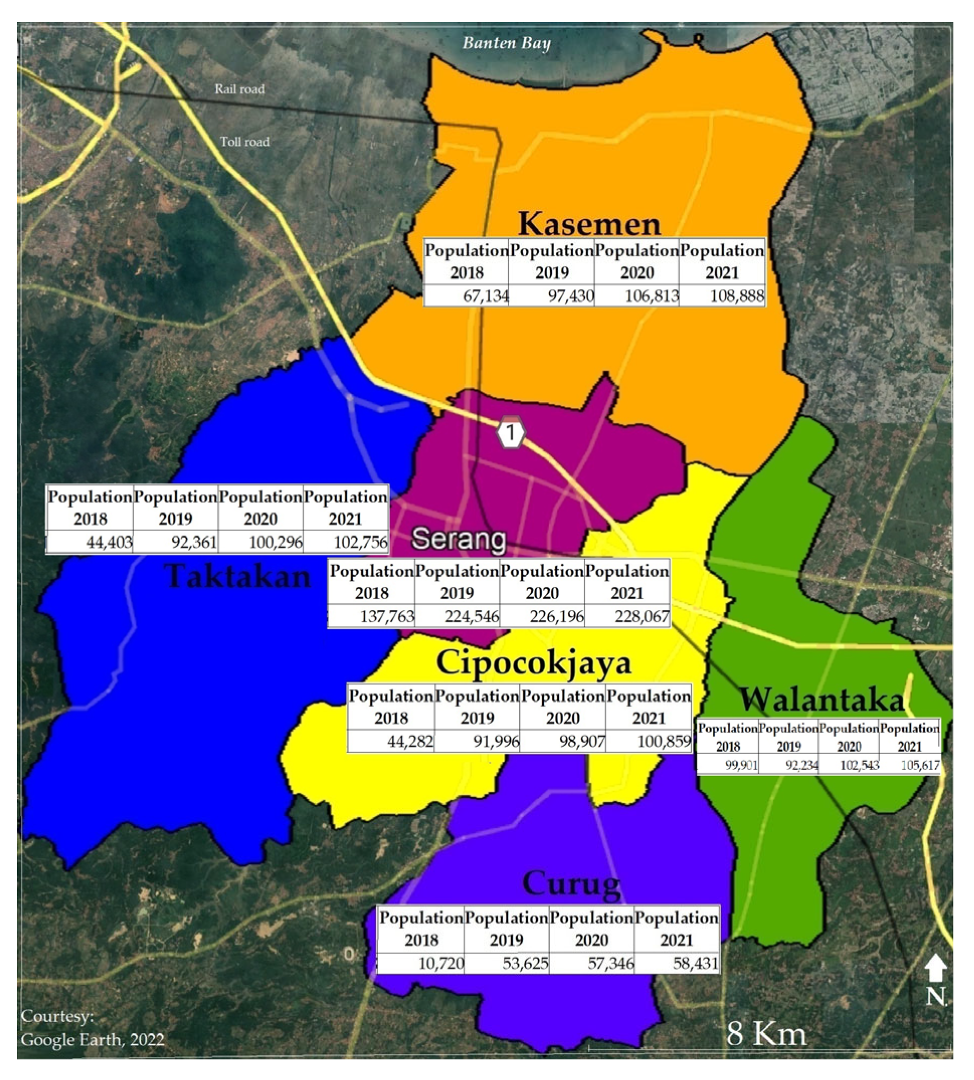
This study used data from Twitter users in the city of Serang in Banten Province, with a population of 687,881 (2021). The city is connected to Jakarta, Indonesia’s capital and the nearest city, by a 71 km toll road to the east. Geographically, the upper limits of the city are at coordinates (−6.014731°, 106.066197°) and (−6.014731°, 106.271097°), while the city’s lower limits are at coordinates (−6.218933°, 106.066197°) and (−6.218525°, 106.271097°). Based on Universal Transfer Mercator (UTM) Zone 48M coordinates, the city area stretches from coordinates 618,000 m in the east to 638,600 m and 9,335,052 m to 9,312,475 m in the south. Thus, the approach size of the city is 20,600 m × 25,250 m.
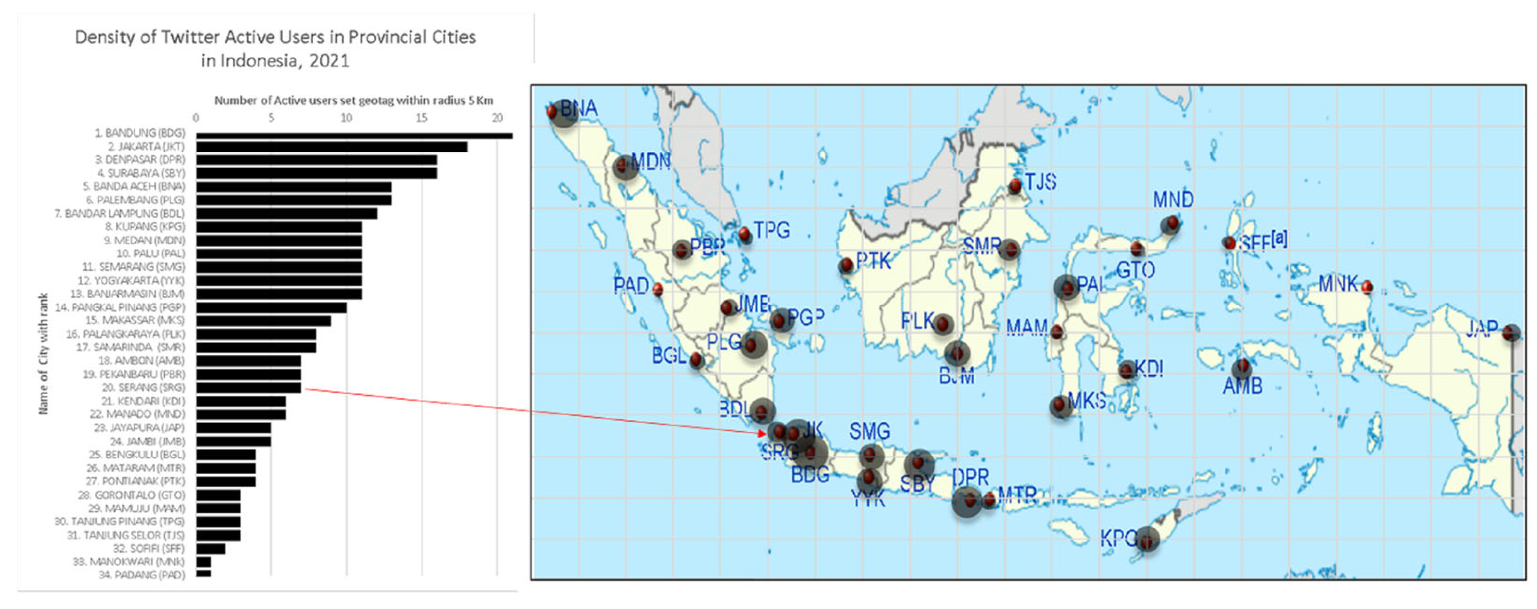
Indonesia has a population of 272.23 million (2020) with 15.7 million Twitter users, as of July 2021 [8]. According to the portrait of data taken and using the program developed for this research, in the first week of July 2021, Serang was among the top 10 cities in Twitter density (with seven users), which is the same amount as in the cities of Pekanbaru and Ambon. Among 34 provincial cities in Indonesia, the highest density of Twitter users was in Bandung (with 21 users) and the least was in Padang (with 1 user). These cities were in the top 16, as shown in Figure 1. Twitter density is defined as the number of active users using geotagged setting within a 5 km area. Thus, Serang is in the medium rank of Twitter user density ranking of Indonesia’s provincial cities.
Twitter data retrieval began on 28 May 2020. The target goal was to determine the total number of Twitter users in Serang and their data, which needed to be representative of all analysis zones within the city. The analysis zones followed the administrative areas, or subdistricts, as shown in Figure 2. Twitter data retrieval stopped on 30 April 2021 after sufficient data were collected that was representative of all six analysis zones.
Python script 3.7.4 [30] was used for Twitter data retrieval and was run with Spyder version 5.4.1 under Anaconda3, which is specifically built for this type of research. Anaconda3-navigator version 2.4.0 is a free, open source software distributed by Python and R programming languages [4]. Spyder is also free, open source software and is effective as a cross-platform integrated environment (IDE) for scientific programming using Python [5]. The program can be run on a laptop with the following specifications: Intel®Core™ i3 330M Central Processing Unit (CPU) @ 2.13 Gigahertz (GHz), 3 gigabyte (GB) Random Access Memory (RAM), 32-bit operating system, or Intel®Core™ i7-3520M CPU @ 2.90 GHz, 8 GB RAM, 64-bit operating system, or higher. Retrieved data were stored on MongoDb, an open source database platform; this method for treating Big Data has been recommended by Martin, et al., 2019 [31] and Antonokaki et al., 2021 [32].
3.2. Method
3.2.1. Data Retrieval Techniques
Due to the advantages of open-source nature of Python-based programs, many scholars choose to utilize them for data mining practices, topic modeling, and data analysis [33]. A Spyder Python program has been constructed with consideration of aimed type data, geographical area, time interval, and potential number of retrieved data.
Potential Twitter data content was first determined; this included username, coordinates of the tweet location within the study area and its surroundings, time of tweet, and text of tweet. Secondly, data streaming retrieval was performed using standard API v2. It was necessary to first register for a developer account and create a project on the developer portal. Having once opened a developer account, it was possible to obtain active keys and tokens, and after having registered a new project, it was possible to obtain bearer tokens [3]. The project registered was: “Home-based Trip Production Modeling using LBSN Data”, with an application entitled “Serang Trip Production”. The consumer keys, consumer secret, access key, access secret, and bearer tokens were received.
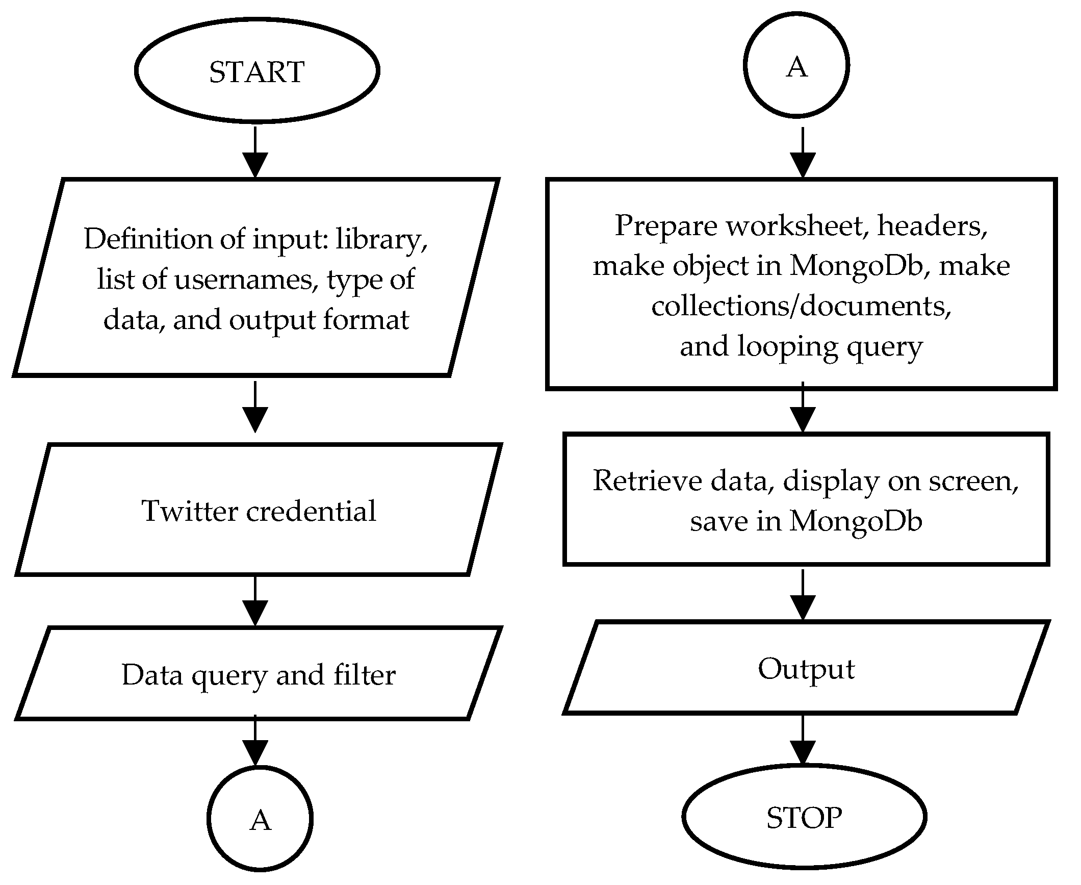
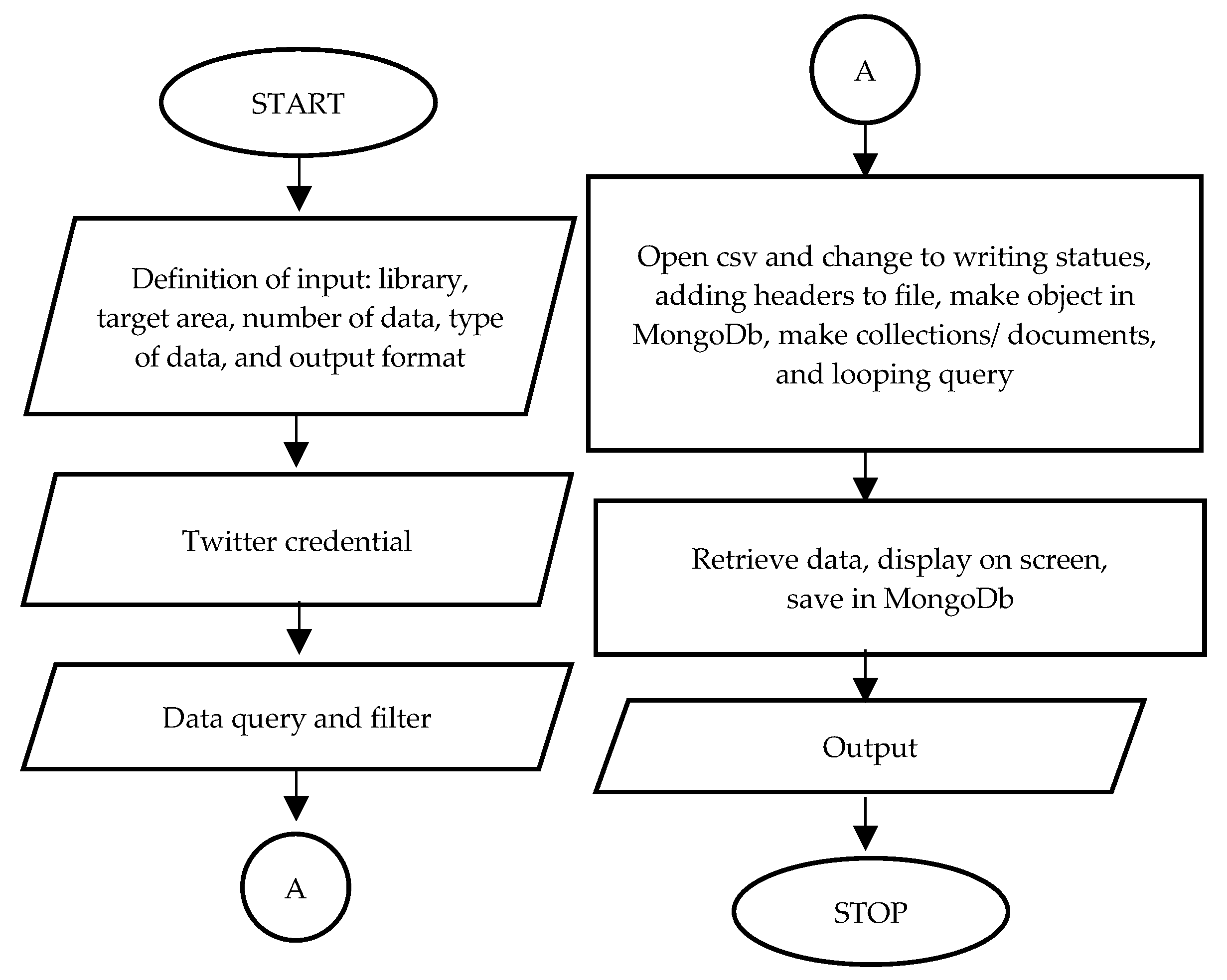
Thirdly, an algorithm was developed for the data retrieval program. The problem formulation of the algorithm for the data streaming retrieval program was to obtain data from within the study area: who, when, where, and whether the tweet was about something related to his/her statues and trip. To retrieve the streaming data, it was necessary to define the input as the coordinate of the target location and the captured area as its radial. The algorithm for the streaming data retrieval program is shown in Figure 3. The program formulation for the algorithm of the archive data retrieval program was to obtain historical data of the users: when, where, and whether the tweet was about something related to his/her statues and trip. For archive data retrieving, it was necessary to define the input as a list of usernames, but there was no need to mention the location coordinates of the target area or apply bearer tokens as part of the access keys. The algorithm for the archive data retrieval program is shown in Figure 4.
Fourthly, a script program for retrieving streaming data was constructed using Python coding, as shown in Attachment S1 (Supplementary Materials). The program was designed to filter geotagged data in decimal degree format. The following information was retrieved: username, Uniform Resource Locator (URL), timestamp, location stamp (latitude, longitude), coordinates in Google Maps, and tweets. The amount of data that needed to be acquired included coordinates of the reference point and the radius of the captured data from the reference point. The extended tweet mode was used in order to get the full text of tweets that contained more than 140 characters. The program was set to save retrieved data in MongoDb.
Fifth, a script program for retrieving historical data was constructed, using Python coding, as shown in Attachment S2 (Supplementary Materials). Similar to retrieving streaming data, the following information was retrieved: username, URL, timestamp, location stamp (latitude, longitude), coordinates in Google Maps, and the tweets. The difference between the two streaming data techniques were the references, i.e., the username of the retrieved data (not the location); and the criteria, i.e., allow both geotagged and non-geotagged data. Twitter usernames to be retrieved were listed as the results of streaming data. A subprogram, Splitter.py, was constructed for the purpose of reading the list (Attachment S3 in Supplementary Materials), and the timeframe of the data was also defined. To identify the results of the streaming data, the URL of the username was set as https://Twitter.com/(username) (access on 30 May 2020 until 30 April 2021), while Twitter.com/(username) was used for archive data (access on 1 May 2021 until 30 September 2021). The program was set to save the retrieved data in MongoDb. A subprogram, Sheet.py, was constructed for saving in MongoDb. (Attachment S4 in Supplementary Materials).
Sixth, the program was run regularly, particularly for data streaming acquisition. Twitter has a data acquisition quota limit of a maximum of 50 data every 15 min; therefore, data collection was repeated accordingly. Data acquisition stops when the Twitter platform has detected that data retrieval has exceeded the limit set. Archive data acquisition was performed using a list of 2492 Twitter usernames that resulted from the acquisition of streaming data. Data acquisition at the initial stage was repeated several times; however, this was not performed for usernames in the archive data acquisition after the same data were obtained.
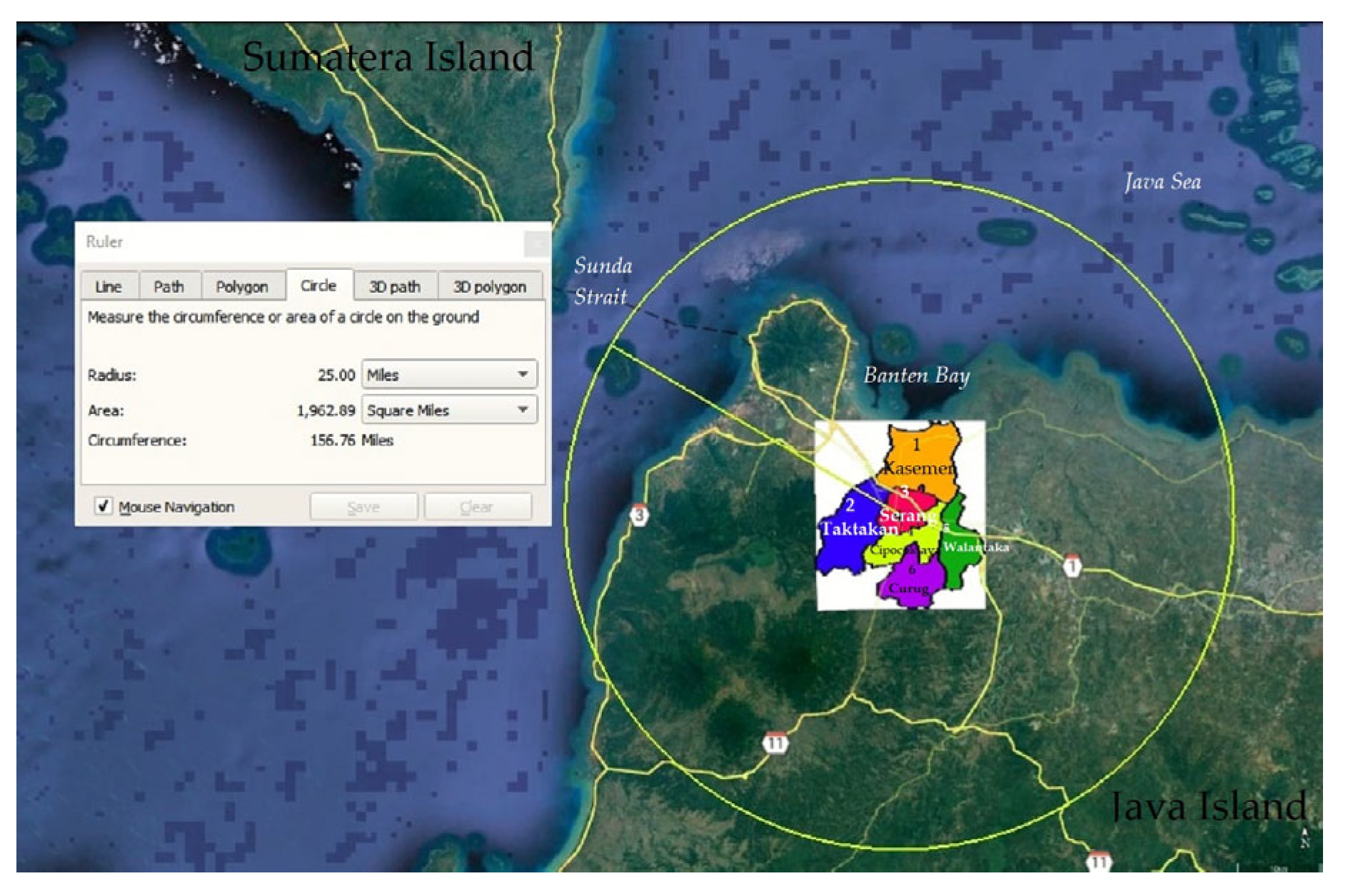
In accordance with the rules for the maximum radius of data coverage, which is 40.2 km, it was assumed that the entire city of Serang, measuring 20.6 km × 25.25 km, could be covered, as shown in Figure 3. At the initial stage, an attempt was made to collect Twitter streaming data using 1 as the reference point for capturing the entire research area at once. The time interval for data acquisition was performed at the same relative time. An attempt was then made to collect data from numerous reference points to capture the entire research area, section by section. Since this revealed more results, using multiple reference points to acquire data was continued. In referring to many reference points, the researchers used the coordinate points of the location of the ward office in each zone, according to subdistrict areas, as shown in Figure 5. The ward offices were: 1. Kasemen, 2. Taktakan, 3. Serang, 4. Cipocokjaya, 5. Walantaka, and 6. Curug.
3.2.2. Utilization of the Scikit-Mobility Python Library for Zonal Trip Production Line
This subsection demonstrates the process of ensuring that all captured data accurately reflects the zonal data in the study area. To predict home locations based on Twitter data, we employed the scikit-mobility (Skmob) library version 0.4.0, a proven python library for mobility data analysis [34]. Skmob offers a range of feature for mobility analysis, such as statistical laws of mobility, generative models, standard pre-processing functions, and methods to assess privacy risk in mobility data [3].
For estimating an individual’s home location based on longitudinal data, Skmob utilizes the Trajectory Data Frame (TrajDataFrame) data structure, which we applied in our analysis. Additionally, we implemented a rule to determine at-home time for night rest between 21:01 and 06.00, with the following script:
- home_location_df=home_location(tdf, start_night=‘21:01’, end_night=‘06:00’, show_progress=True)
4. Results and Compilation
4.1. Results from Data Streaming Retrieving Technique
Data from a total of 2491 Twitter users were captured in the research area of Serang City during the data collection period from 30 May 2019 to 30 April 2021.
4.1.1. Data Acquisition Using a Single Reference Point
By setting the Twitter data collection point at the midpoint of Serang, based on a four-square approach: P (−6.116897°, 106.15948°). Note: hereafter, the notations will be in decimal degrees. An experiment was conducted to adjust the range to obtain as many data as possible for each acquisitioning cycle. The results for each Twitter data acquisition, using a single reference point with different capturing distances, are shown in Table 1.
A setting of 100 or 50 data was used in the single reference point method each time; the maximum amount of data obtained was 15 unique data. A setting of 50 was used for data collection for each complete iteration in the program. As a result, there was a large amount of data duplication that needed to be discarded. When the distance was set with an integer of 1, or another integer, to a limit of 5 km, the same number of unique data was obtained, which was 15. However, setting distances of 1 and 2 km produced only 1 location, representing all user locations; this was termed a cluster. Setting distances of 3, 4, and 5 km produced as much as three clusters. The term “cluster” in this paper indicates a point representing the location of many users, or a single user at different times but at the same location. Thus, to obtain the maximum number of clusters, the capturing distance would need to be set at 3, 4, or 5 km; however, the amount of target data does not need to be as high as 50. It was found that the data obtained was at a distance that exceeded the capturing distance setting number.
4.1.2. Data Retrieving Using Multi-Reference Points
For the entire study area, 65 reference points (RPs) were obtained based on the location of the ward office in each subdistrict: Cipocokjaya—8 points; Curug—10 points, Kasemen—10 points, Serang—11 points, Taktakan—12 points; and Walantaka—14 points. The results of streaming data retrieving using multi-references with a capturing distance 3 km, for example, that of Cipocokjaya, is shown in Table 2.
Data retrieving using both techniques was carried out on the same day. Comparing the results of using single reference points with the results of multi-reference points, it was found that more unique data were obtained, as well as more locations and a greater number of users.
The location points of cluster data always exceed the capturing distance set in the script program. The use of multiple reference points, as in the example above where there are eight points, makes it possible to obtain data for 7 (seven) unique cluster data location points. These include:
−6.172153, 106.127458; −6.148666,106.127825;
−6.176018, 106.196267; −6.20948,106.129581;
−6.173101, 106.071077; −6.134538,106.167998;
−6.137688, 106.13405.
In capturing data streaming, it can be seen that the use of multiple reference points produces more spatial data as opposed to the use of one reference point. A list of the usernames within the study area was also obtained, along with a number of his/her geotagged data during the data collection time. For trip production modeling purposes, a basic rule can be made regarding the number of geotagged data figuring his/her origin and the trip to work for at least two different locations, where two geotagged data in the same zone of the study area and two other data from elsewhere. Each datum must have a different date.
By using data streaming retrieval with multi-reference points, we retrieved data from 2491 users. The data show that 416 (54%) had only one location, 249 (32%) had two locations, 70 (9%) had three locations, and 47 (5%) had four or more locations.
4.2. Results from Archive Data Retrieving Technique
Data from a total of 506 Twitter users in 2018, 742 Twitter users in 2019, 1632 Twitter users, and 1032 Twitter users in 2021 were obtained through the Archive Data Retrieving Technique. Archive data acquisition was performed using a list of 2491 usernames from the acquisition of streaming geotagged data to obtain additional data. The program was set for a yearly acquisition time, from 1 January 2018 to 30 April 2021. After all cycles of running the program, 2827 geotagged data and 520,272 nongeotagged data were obtained (Table 3). According to archive data captured, not all users’ geotagged data available.
The archival data were intended for data modeling purposes, and were collected to compare and contrast with the trip production model based on conventional data (household surveys and roadside interviews) that were gathered in 2018.
4.3. Data Compilation
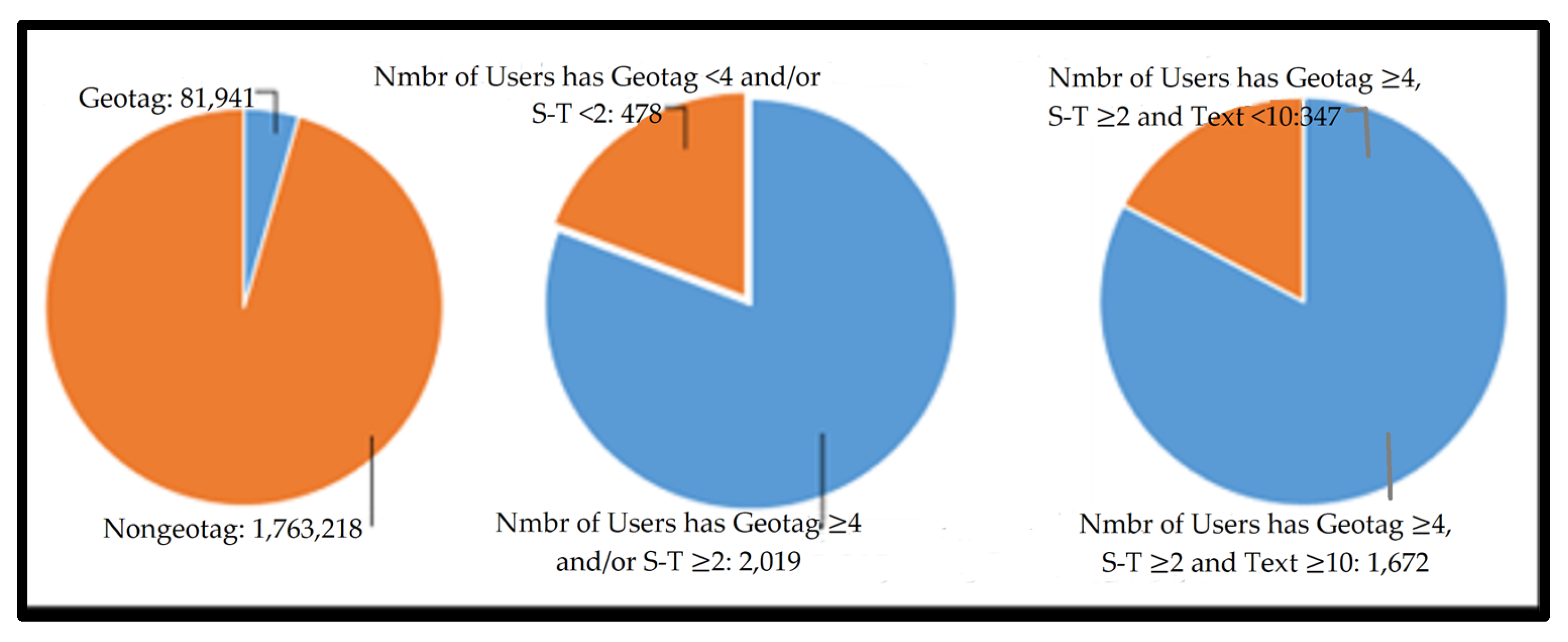
Data compilation results from data acquisition using both methods are as follows. So far, 1,763,218 nongeotagged data have been obtained, compared to 81,941 geotagged data obtained from 2491 users (Figure 6). The database consisted of 2491 collections; these needed to have duplications of document in each collection filtered out, as well as out-of-range data in terms of area and time. PyCharm software Community Edition version 2019.1.2 was used to edit every document in each collection in order for these to be readable by the Python-based program in the filtering process. Among the geotagged data, with respect to the source of data, there were 21,996 (40.6%) data from streaming and 32,152 (59.4%) from archiving.
Among a collection of 1769 users that met the statistical requirements (geotagged data ≥ 4), only 29% of the data collection from streaming data and 41% of data collection met the statistical rules; this was due to additional data coming from archive data. Thus, archive data can make a significant contribution to readiness data for trip production modeling.
A large amount of data has been archived as these showed tweets with multipoints and not just one point as in streaming data. (See example below). Documents #1 (Table 4) and #2 (Table 5) provide the coordinates of two locations of the same tweet from archive data within a distance of about 4.7 km; neither of these have the same location coordinates from streaming data, as seen in Document #3 (Table 6). These data show inconsistency in the location where the tweets took place.
A large amount of archive data were also obtained that showed tweets with a different date and month timestamp compared to the same tweet from streaming data. However, it was intuitively determined to be the same timestamp, as can be seen in the example below. Document #1 has archive data stamped 12 June, and document #2 has streaming data stamped 6 December having the same year, clock hour, and minute. Since the Twitter platform only gives access to streaming data from the previous seven days, it was impossible to pull data from as far back as 12 June 2020.
For trip production modeling, textual data were collected from both streaming and archive data; some of these tweets were not from the user him/herself, but from others, as seen in the example below. As actual expressions/opinions/judgments from the account users were needed, it became necessary to omit text tweets from others and maximize the number of tweets with text that were directly from the account user.
Document #1 contains tweet texts without the name of the account username. The user mentions his opinion about his transportation difficulties in the city. Document #2 includes the same name as the account username (@Rizkasyarahr), indicating that he had received information that was not from the user himself.
4.4. Zonal Data
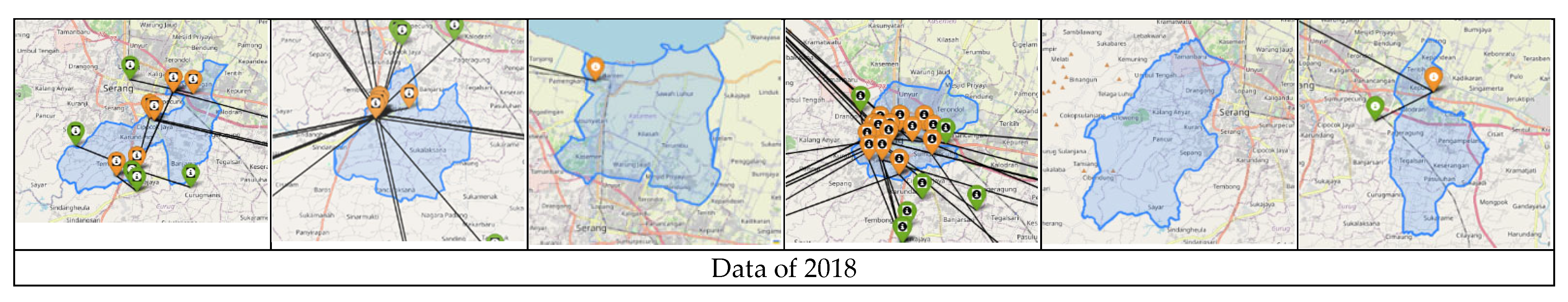
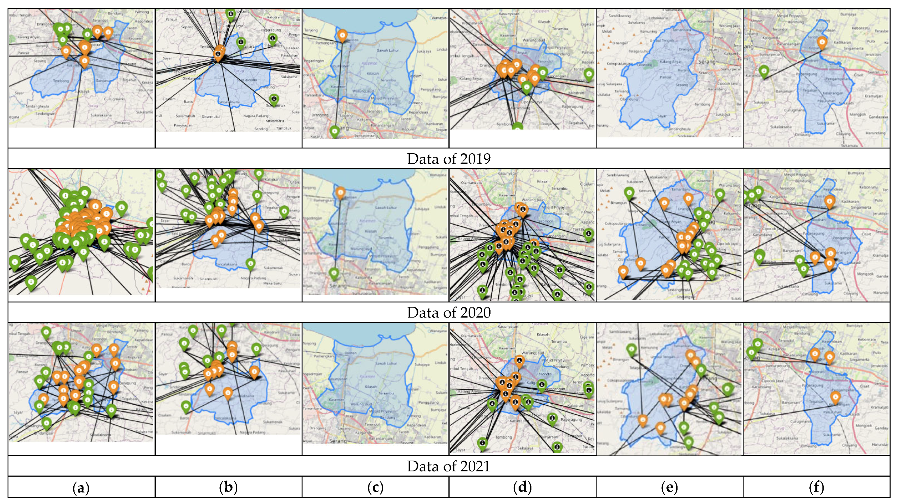
Figure 7 demonstrates that the techniques employed in this study are able to capture data representing all six zones in the study area. We split the data on a yearly basis to illustrate the availability of data concerning the zonal trip production pattern. Each figure represents the vector of a zone to produce home-based trip for work purpose.
By presenting the predicted trip lines for each production zone in the years 2018, 2019, 2020, and 2021, we highlight the evolution of travel patterns and the effectiveness of our modeling approach. The yellow bullets on the maps represent home locations, while the green bullets indicate work locations in proximity to the respective zones. Among all six zones, Zone 1 emerges as the most productive zone in 2021, whereas Zone 3 exhibits the least productivity. Notably, Zone 3 shows minimal development from 2018 to 2021, whereas Zone 5 demonstrates significant development during this period.
These maps serve as visual evidence that our study has successfully achieved its aim of developing trip production models using LBSN data.
5. Discussion
For the purpose of researching urban passenger trip production modeling, a retrieving program for data streaming was set up with specific coordinates of target location and distance limitations. When using archive data retrieving, the reference is username, not the coordinates of the target location, which would make it possible to get multiple geotags of the same tweet. This study was concerned with obtaining fixed geotags in order to obtain accurate single locations. The text content of the tweet can serve as potential raw data for inferring user labels such as: social status, gender, age group, and marital status, as well as economic status, occupation, vehicle usage, and travel purposes. Area conditions that relate to travel can also be inferred, such as traffic conditions, road conditions, and conditions of access to public transportation.
Having multipoints of a tweet location from archive data helps create awareness about location bias and further calculations based regarding this. Thus, it is important to refer to related research by Yang and Eickhoff (2018) [35] and Ozdikis, et al. (2019) [36]. Yang and Eickhoff were concerned about multipoints of check-in locations and made a representative coordinate centroid. Ozdikis, et al. used the coordinate location of users, based on centroid coordinates of predicted, non-geotagged tweet locations. This study proposes the use of centroid coordinates based on the average latitude/longitude location stamps of a tweet as proxy for the user coordinate location at the time.
By having multidates of tweet time from archive data and streaming data, this study proposes the use of a date according to the timestamp of the streaming data. Valid timestamp data are crucial for predicting user label activity and location based on the text of the tweet and the timestamp, as mentioned.
For the purpose of labeling the user account, the tweet message containing @(user account name) does not reflect the user’s own description; thus, it was not necessary to keep the data which could be removed from the dataset to make the database smaller. For other research purposes, text messages from user networking could be of value, such as has been elaborated by Chen, et al. (2016) [37] and Fang, et al. (2017) [38], who used the perspective of transportation.
6. Conclusions
Twitter data, from streaming and archive, can be retrieved using a Spyder Python-based program. Twitter archive data were obtained by using API Research, which was rich in textual data, but lacking in geotagged data, compared to the Twitter streaming data obtained when using API Standard v2. Using Twitter data extraction made it possible to obtain location and text data from Twitter users continuously, although this was limited in accordance with regulations set by Twitter.
Twitter data retrieval for home-based work (HBW) trip production modeling needs unique algorithms that are based on the data needed. For HBW trip production modeling, Twitter geotagged data are important, not only for estimating location and time of trip departure and/or destination, but also for estimating labels of the trip maker’s attributes and location, such as home or elsewhere. Since calculating an individual trip requires two coordinate locations, a minimal number of individual geotagged data from within the study area are needed. Twitter data retrieving using API Research does not capture enough geotagged data; thus, it is necessary to use both API Research and API Standard v2. This can be performed by first completing streaming data retrieval using API Standard v2 and obtaining a list of Twitter users within a particular study area. Archive data retrieval can then be applied, using API Research.
Retrieving streaming data using multi-reference locations representing residential area within a particular zone gives more captured data than using one reference location. Intermittently running the program for an interval time, based on data occurrence, such as 20–30 min, is recommended.
Instead of using data from both categories of data collection, data streaming data, and data archive, data streaming must be made with a time reference for any data identified as having same tweet content. For any tweet data identified as having the same tweet content and timestamp, but different location coordinates, thus showing inconsistent coordinates, the central location needs to be determined. For the most efficient data preprocessing, it is better to ensure there is enough data collection by using streaming data retrieving. For updating a data collection, it is recommended to retrieve data using streaming data.
The Twitter data retrieving technique presented in this paper can be applied to Twitter data retrieval not only in the city of Serang, but also in other regions of Indonesia and any place in the World, according to Twitter’s current data access policy and procedures, particularly for academic research. The explanation of Twitter data retrieving techniques in this paper has the potential to be widely recognized among scholars and provide researchers with more opportunities for using Twitter data in transportation demand modeling. As long as Twitter maintains an open data policy regarding its database, and Twitter data collection for research purposes is not considered a violation of personal data protection laws or the like, further research on data mining for transportation demand modeling remains widely accessible.
Through the results presented in Section 3, we have demonstrated the potential and applicability of mining LBSN data for trip production modeling and its relevance to broader fields such as passenger transportation demand modeling. Our findings provide guidance for transportation system researchers and data scientists in further studies utilizing LBSN data.
This study contributes to the literature of advanced research on transportation demand modeling in terms of LBSN data. The Twitter data retrieval technique used in this research is the initial part involved in modeling the production of user journeys using machine learning. Data retrieval results still need to be processed to be readable by the program developed for modeling. In order for the program to run, the following components are needed: a modeling program based on machine learning, a computer environment, and collaboration with programmers. Thus, it can be seen that the development of transportation science is leading to the adoption of machine learning and a greater understanding of the policies of location-based social network platform providers. On the other hand, with the potential for obtaining and processing large amounts of data sources in a relatively short time at low costs, travel production calculations in a specific area can be carried out more frequently in order to improve transportation services and urban activities.
Supplementary Materials
The following supporting information can be downloaded at: https://www.mdpi.com/article/10.3390/app13148539/s1.
Author Contributions
Conceptualization, R.S.R. and H.P.H.P.; Data curation, R.S.R.; Formal analysis, R.S.R. and P.D.; Investigation, R.S.R. and H.P.H.P.; Methodology, R.S.R., A.D., H.P.H.P. and P.D.; Project administration, R.S.R.; Resources, R.S.R.; Supervision, A.D., H.P.H.P. and P.D.; Validation, H.P.H.P.; Visualization, R.S.R.; Writing—original draft, R.S.R.; Writing—review and editing, R.S.R. All authors have read and agreed to the published version of the manuscript.
Funding
Research was supported by Ganesha Talent Assistantship, Bandung Institute of Technology (Decree Number: 263B/IT1.A/SK/DA/2020).
Institutional Review Board Statement
All data were available publicly under an open license and therefore exempt from institutional review board review.
Informed Consent Statement
All data were available publicly under an open license and therefore exempt from informed consent statement.
Data Availability Statement
The identified data is available upon request.
Acknowledgments
The writing of this manuscript was assisted by the Writing Scientific Articles Coaching Team, School of Architecture, Planning and Policy Development, Institute of Technology Bandung. All Python script programs used in this research study were developed by Richard Shiawase.
Conflicts of Interests
The authors hereby declare that there were no competing financial, professional, or personal interests that might have influenced the development or presentation of this research work.
Internet List:
- 1.
- https://developer.twitter.com/en/docs/twitter-api/rate-limits (accessed on 22 September 2020)
- 2.
- https://developer.twitter.com/en/docs/tutorials/filtering-tweets-by-location (accessed on 22 September 2020)
- 3.
- https://developer.twitter.com/en/docs/tutorials/stream-tweets-in-real-time (accessed on 22 September 2020)
- 4.
- https://anaconda.org/ (accessed on 17 December 2018)
- 5.
- https://docs.spyder-ide.org/current/index.html (accessed on 17 December 2018)
- 6.
- https://developer.twitter.com/en/products/twitter-api/academic-research/application-info (accessed on 22 September 2020)
- 7.
- https://developer.twitter.com/en/docs/twitter-api/search-overview (accessed on 22 September 2020)
- 8.
- https://databoks.katadata.co.id/datapublish/2021/11/04/ (accessed on 22 September 2020)
References
- Zhang, X.; Xu, Y.; Tu, W.; Ratti, C. Do different datasets tell the same story about urban mobility—A comparative study of public transit and taxi usage. J. Transp. Geogr. 2018, 70, 78–90. [Google Scholar] [CrossRef]
- Golder, S.A.; Macy, M.W. Digital Footprints: Opportunities and Challenges for Online Social Research. Annu. Rev. Sociol. 2014, 40, 129–152. [Google Scholar] [CrossRef] [Green Version]
- Pappalardo, L.; Simini, F.; Barlacchi, G.; Pellungrini, R. Scikit-mobility: A Python Library for the Analysis, Generation, and Risk Assessment of Mobility Data. J. Stat. Softw. 2022, 103, 4. [Google Scholar] [CrossRef]
- Milne, D.; Watling, D.P. Big data and understanding change in the context of planning transport systems. J. Transp. Geogr. 2017, 76, 235–244. [Google Scholar] [CrossRef]
- Hasnat, M.M.; Hasan, S. Identifying tourists and analyzing spatial patterns of their destinations from location-based social media data. Transp. Res. Part C 2018, 96, 38–54. [Google Scholar] [CrossRef]
- Llorca, C.; Ji, J.; Molloy, J.; Moeckel, R. The usage of location based big data and trip planning services for the estimation of a long-distance travel demand model. Predicting the impacts of a new high speed rail corridor. Res. Transp. Econ. 2018, 72, 27–36. [Google Scholar] [CrossRef]
- Yang, F.; Li, L.; Ding, F.; Tan, H.; Ran, B. A data-driven approach to trip generation modeling for urban residents and non-local travelers. Sustainability 2020, 12, 7688. [Google Scholar] [CrossRef]
- Hu, W. Dynamic Origin Destination Estimation with Location-Based Social Networking Data: Exploring Urban Travel Demand Sensor; The State University of New Jersey: New Brunswick, NJ, USA, 2019. [Google Scholar]
- Hasnat, M.M.; Faghih-Imani, A.; Eluru, N.; Hasan, S. Destination choice modeling using location-based social media data. J. Choice Model. 2019, 31, 22–34. [Google Scholar] [CrossRef]
- De Ortúzar, J.D.; Willumsen, L.G. Modelling Transport, 4th ed.; John Wiley & Sons: Chichester, UK, 2011. [Google Scholar]
- Cordera, R.; Coppola, P.; Dell’Olio, L.; Ibeas, Á. Is accessibility relevant in trip generation? Modelling the interaction between trip generation and accessibility taking into account spatial effects. Transportation 2017, 44, 1577–1603. [Google Scholar] [CrossRef]
- Shafie, S.A.B.M.; Sadullah, A.F.M.; Hamzah, M.O.; Leong, L.V. The Alternative Trip Generation Model for Flat/Apartment/Condominium and Low Cost Housing Subcategories. Appl. Mech. Mater. 2015, 802, 369–374. [Google Scholar] [CrossRef]
- Shi, F.; Zhu, L. Analysis of trip generation rates in residential commuting based on mobile phone signaling data. J. Transp. Land Use 2019, 12, 201–220. [Google Scholar] [CrossRef]
- Kröger, L.; Heinitz, F.; Winkler, C. Operationalizing a spatial differentiation of trip generation rates using proxy indicators of accessibility. Travel Behav. Soc. 2018, 11, 156–173. [Google Scholar] [CrossRef]
- Chang, J.S.; Jung, D.; Kim, J.; Kang, T. Comparative analysis of trip generation models: Results using home-based work trips in the Seoul metropolitan area. Transp. Lett. 2014, 6, 78–88. [Google Scholar] [CrossRef] [Green Version]
- Hedau, A.L.; Sanghai, S.S. Development of Trip Generation Model Using Activity Based Approach. Int. J. Civil Struct. Environ. Infrastruct. Eng. 2014, 4, 61–78. [Google Scholar]
- Guzman, L.A.; Gomez, A.M.; Rivera, C. A Strategic Tour Generation Modeling within a Dynamic Land-Use and Transport Framework: A Case Study of Bogota, Colombia. Procedia Transp. Res. 2017, 25, 2536–2551. [Google Scholar] [CrossRef]
- Cui, Y.; Meng, C.; He, Q.; Gao, J. Forecasting current and next trip purpose with social media data and Google Places. Transp. Res. Part C Emerg. Technol. 2018, 97, 159–174. [Google Scholar] [CrossRef]
- Qian, C.; Kats, P.; Malinchik, S.; Hoffman, M.; Kettler, B.; Kontokosta, C.; Sobolevsky, S. Geo-tagged social media data as a proxy for urban mobility. Adv. Intell. Syst. Comput. 2018, 610, 29–40. [Google Scholar]
- Pourebrahim, N.; Sultana, S.; Niakanlahiji, A.; Thill, J.-C. Trip distribution modeling with Twitter data. Comput. Environ. Urban Syst. 2019, 77, 101354. [Google Scholar] [CrossRef]
- Bakerman, J.; Pazdernik, K.; Wilson, A.; Fairchild, G.; Bahran, R. Twitter Geolocation: A Hybrid Approach. ACM Trans. Knowl. Discov. Data 2018, 12, 34:1–34:17. [Google Scholar] [CrossRef]
- MacEachren, A.M.; Jaiswal, A.; Robinson, A.C.; Pezanowski, S.; Savelyev, A.; Mitra, P.; Zhang, X.; Blanford, J. SensePlace2: GeoTwitter Analytics Support for Situational Awareness. In Proceedings of the 2011 IEEE Conference on Visual Analytics Science and Technology (VAST), Providence, RI, USA, 23–28 October 2011; pp. 181–190. [Google Scholar]
- Burkhalter, J.N.; Wood, N.T. Twitter data acquisition and analysis: Methodology and best practice. In Maximizing Commerce and Marketing Strategies through Micro-Blogging; ANU College of Business and Economics: Canberra, Australia, 2015; pp. 280–296. [Google Scholar]
- McCormick, T.H.; Lee, H.; Cesare, N.; Shojaie, A.; Spiro, E.S. Using Twitter for Demographic and Social Science Research: Tools for Data Collection and Processing. Sociol. Methods Res. 2015, 1, 390–421. [Google Scholar] [CrossRef]
- De, S.; Zhou, Y.; Abad, I.L.; Moessner, K. Cyber–Physical–Social Frameworks for Urban Big Data Systems: A Survey. Appl. Sci. 2017, 7, 1017. [Google Scholar] [CrossRef] [Green Version]
- Russell, M.A. Mining the Social Web, 2nd ed.; O’Reilly: Newton, MA, USA, 2017; pp. 351–397. [Google Scholar]
- Serna, A.; Gerrikagoitia, J.K.; Bernabé, U.; Ruiz, T. Sustainability analysis on Urban Mobility based on Social Media content. Transp. Res. Procedia 2017, 24, 1–8. [Google Scholar] [CrossRef]
- lvaro Cuesta, Ã.; Barrero, D.F.; R-Moreno, M.D. A framework for massive twitter data extraction and analysis. Malays. J. Comput. Sci. 2014, 27, 50–67. [Google Scholar]
- Al Bashaireh, R.; Zohdy, M.; Sabeeh, V. Twitter Data Collection and Extraction: A Method and a New Dataset, the UTD-MI. In Proceedings of the 2020 the 4th International Conference on Information System and Data Mining, Hawaii, HI, USA, 15–17 May 2020; pp. 71–76. [Google Scholar]
- Haupt, M.R.; Jinich-Diamant, A.; Li, J.; Nali, M.; Mackey, T.K. Characterizing twitter user topics and communication network dynamics of the ‘Liberate’ movement during COVID-19 using unsupervised machine learning and social network analysis. Online Soc. Netw. Media 2021, 21, 100114. [Google Scholar] [CrossRef]
- Martín, A.; Belén, A.; Julián, A.; Cos-gayón, F. Analysis of Twitter messages using big data tools to evaluate and locate the activity in the city of Valencia (Spain). Cities 2019, 86, 37–50. [Google Scholar] [CrossRef]
- Antonakaki, D.; Fragopoulou, P.; Ioannidis, S. A survey of Twitter research: Data model, graph structure, sentiment analysis and attacks. Expert Syst. Appl. 2021, 164, 114006. [Google Scholar] [CrossRef]
- Abdul-Rahman, M.; Chan, E.H.W.; Wong, M.S.; Irekponor, V.E.; Abdul-Rahman, M.O. A framework to simplify pre-processing location-based social media big data for sustainable urban planning and management. Cities 2021, 109, 102986. [Google Scholar] [CrossRef]
- Yu, Q.; Yuan, J. TransBigData: A Python package for transportation spatio-temporal big data processing, analysis and visualization. J. Open Source Softw. 2022, 7, 4021. [Google Scholar] [CrossRef]
- Yang, J.; Eickhoff, C. Unsupervised Learning of Parsimonious General-Purpose Embeddings for User and Location Modeling. ACM Trans. Inf. Syst. 2018, 36, 1–33. [Google Scholar] [CrossRef]
- Ozdikis, O.; Ramampiaro, H.; Nørvåg, K. Locality-adapted kernel densities of term co-occurrences for location prediction of tweets. Inf. Process. Manag. 2019, 56, 1280–1299. [Google Scholar] [CrossRef]
- Chen, C.; Ma, J.; Susilo, Y.; Liu, Y.; Wang, M. The promises of big data and small data for travel behavior (aka human mobility) analysis. Transp. Res. Part C 2016, 68, 285–299. [Google Scholar] [CrossRef] [PubMed] [Green Version]
- Fang, Z.; Yang, X.; Xu, Y.; Shaw, S.; Yin, L. Spatiotemporal model for assessing the stability of urban human convergence and divergence patterns. Int. J. Geogr. Inf. Sci. 2017, 31, 2119–2141. [Google Scholar] [CrossRef]
Figure 1.
Density of Twitter Users in Provincial Cities in Indonesia, 2021. Source: Data retrieving, 1 and 2 July 2021.
Figure 1.
Density of Twitter Users in Provincial Cities in Indonesia, 2021. Source: Data retrieving, 1 and 2 July 2021.

Figure 2.
Study Area: City of Serang and its six subdistricts.

Figure 3.
Algorithm for Twitter streaming data retrieval.

Figure 4.
Algorithm for Twitter archive data retrieval.

Figure 5.
Positioning of research area within 25 miles (40.2 km) and the locations of ward offices. Source: plotting points and boundaries on Google Earth.
Figure 5.
Positioning of research area within 25 miles (40.2 km) and the locations of ward offices. Source: plotting points and boundaries on Google Earth.

Figure 6.
Availability of Twitter Data for Trip Production Modeling of Serang City.

Figure 7.
Predicted Trip Lines for Each Production Zone of Serang City, 2018–2021. (a) Z-1:Cipocokjaya. (b) Z-2:Curug. (c) Z-3:Kasemen. (d) Z-4:Serang. (e) Z-5:Taktakan. (f) Z-6:Walantaka.
Figure 7.
Predicted Trip Lines for Each Production Zone of Serang City, 2018–2021. (a) Z-1:Cipocokjaya. (b) Z-2:Curug. (c) Z-3:Kasemen. (d) Z-4:Serang. (e) Z-5:Taktakan. (f) Z-6:Walantaka.


Table 1.
Results of Twitter data retrieving using single reference point.
| # | (1) | (2) | (3) | (4) | (5) | (6) |
|---|---|---|---|---|---|---|
| 1 | 1 | kota_2036170820.csv | 15 | 11 | 1 | −6.148666°, 106.127825° (6.00) |
| 2 | 2 | kota_2041170820.csv | 15 | 11 | 1 | −6.148666°, 106.127825° (6.00) |
| 3 | 3 | kota_2031170820.csv | 15 | 12 | 3 | −6.173101°, 106.071077° (11.59) |
| 4 | 4 | kota_2044170820.csv | 15 | 12 | 3 | −6.173101°, 106.071077° (11.59) |
| 5 | 5 | kota_2045170820.csv | 15 | 12 | 3 | −6.173101°, 106.071077° (11.59) |
Notes: (1) Capturing distance (km); (2) Source of file name; (3) Number of unique data; (4) Number of user(s); (5) Number of location(s); (6) Farthest point and distance (km).
Table 2.
Twitter data retrieving results using multi-reference points (Example: Cipocokjaya zone).
| # | (1) | (2) | (3) | (4) | (5) | (6) |
|---|---|---|---|---|---|---|
| 1 | −6.154017,106.138792 (3) | Cip1_2204170820.csv | 10 | 5 | 3 | −6.134539, 106.167998 (3.88) |
| 2 | −6.140438,106.147322 (3) | Cip2_2205170820.csv | 13 | 10 | 3 | −6.173101, 106.071077 (9.18) |
| 3 | −6.144682,106.158796 (3) | Cip3_2206170820.csv | 13 | 10 | 3 | −6.173101, 106.071077 (10.20) |
| 4 | −6.144942,106.161058 (3) | Cip4_2207170820.csv | 15 | 8 | 2 | −6.173101, 106.071077 (10.43) |
| 5 | −6.133726,106.173318 (3) | Cip5_2208170820.csv | 15 | 7 | 4 | −6.173101,106.071077 (12.13) |
| 6 | −6.162454,106.181465 (3) | Cip6_2209170820.csv | 15 | 8 | 3 | −6.209480, 106.129581 (7.75) |
| 7 | −6.137307,106.198948 (3) | Cip7_2209170820.csv | 15 | 7 | 4 | −6.173101,106.071077 (14.70) |
| 8 | −6.118432,106.198660 (3) | Cip8_2210170820.csv | 15 | 7 | 3 | −6.173101,106.071077 (15.36) |
| Aggregation: | 47 | 27 | 7 | |||
Notes: (1) Reference Point and Capturing distance (km); (2) Source of file name; (3) Number of unique data; (4) Number of user(s); (5) Number of location(s); (6) Farthest point and distance (km).
Table 3.
Number of Retrieved Archive Data.
| Archive Data | ||||
|---|---|---|---|---|
| 2018 | 2019 | 2020 | 2021 * | |
| Number of Users | 506 | 742 | 1632 | 1032 |
| Number of Geotagged Data | 232 | 476 | 1286 | 833 |
| Number of Nongeotagged Data | 61,825 | 129,300 | 259,253 | 69,894 |
* until 30 April 2021.
Table 4.
Document #1.
| # | (1) | (2) | (3) | (4) | (5) | (6) |
|---|---|---|---|---|---|---|
| 1 | papatonghiber | twitter.com/papatonghiber (accessed on: 8 June 2021) | 8 September 2020 03:46 | −6.17602 | 106.196 | Main dulu ke rumah… (let’s play at my home first…) |
| 2 | papatonghiber | twitter.com/papatonghiber (accessed on: 29 July 2021) | 8 September 2020 03:46 | −6.13197 | 106.196 | Main dulu ke rumah… (let’s play at my home first…) |
| 3 | papatonghiber | https://twitter.com/papatonghiber (accessed on: 8 September 2020 ) | 8 September 2020 03:46 | −6.17222 | 106.162 | Main dulu ke rumah… (let’s play at my home first…) |
Note: (1) Name; (2) Profile URL; (3) Time stamp; (4) Latitude; (5) Longitude; (6) Tweet text.
Table 5.
Document #2.
| # | (1) | (2) | (3) | (4) | (5) | (6) |
|---|---|---|---|---|---|---|
| 1 | onotwitercom | twitter.com/onotwitercom (accessed on: 14 July 2021) | 12 June 2020 09:45 | −6.14867 | 106.1278 | @trans7club Sama disini hujan (@trans7 Here is raining, too) |
| 2 | onotwitercom | https://twitter.com/onotwitercom (accessed on: 12 June 2020) | 12 June 2020 09:45 | −6.09702 | 106.0768 | @trans7 Sama disini juga hujan (@trans7 Here is raining, too) |
Note: (1) Name; (2) Profile URL; (3) Time stamp; (4) Latitude; (5) Longitude; (6) Tweet text.
Table 6.
Document #3.
| # | (1) | (2) | (3) | (4) | (5) | (6) |
|---|---|---|---|---|---|---|
| 1 | Rizkasyarahr | twitter.com/rizkasyarahr (accessed on: 11 August 2021) | 24 April 2021 11:03 | −6.17215 | 106.1275 | b’Asli serang jadi macet bgt. Apa guenya yg jarang keluar rumah ?’ (Obviously Serang is so stuck. Am I the one who rarely leaves home?’) |
| 2 | Rizkasyarahr | twitter.com/rizkasyarahr (accessed on: 9 July 2021) | 16 June 2019 04:32 | - | - | @Rizkasyarahr jadi mau ke Guardian :( (@Rizkasyarahr so you want to go to Guardian :() |
Note: (1) Name; (2) Profile URL; (3) Time stamp; (4) a Latitude; (5) a Longitude; (6) Tweet text.
Disclaimer/Publisher’s Note: The statements, opinions and data contained in all publications are solely those of the individual author(s) and contributor(s) and not of MDPI and/or the editor(s). MDPI and/or the editor(s) disclaim responsibility for any injury to people or property resulting from any ideas, methods, instructions or products referred to in the content. |
© 2023 by the authors. Licensee MDPI, Basel, Switzerland. This article is an open access article distributed under the terms and conditions of the Creative Commons Attribution (CC BY) license (https://creativecommons.org/licenses/by/4.0/).
Share and Cite
MDPI and ACS Style
Rayat, R.S.; Dwicaksono, A.; Putro, H.P.H.; Dirgahayani, P. Applied Techniques for Twitter Data Retrieval in an Urban Area: Insight for Trip Production Modeling. Appl. Sci. 2023, 13, 8539. https://doi.org/10.3390/app13148539
AMA Style
Rayat RS, Dwicaksono A, Putro HPH, Dirgahayani P. Applied Techniques for Twitter Data Retrieval in an Urban Area: Insight for Trip Production Modeling. Applied Sciences. 2023; 13(14):8539. https://doi.org/10.3390/app13148539
Chicago/Turabian StyleRayat, Rempu Sora, Adenantera Dwicaksono, Heru P. H. Putro, and Puspita Dirgahayani. 2023. "Applied Techniques for Twitter Data Retrieval in an Urban Area: Insight for Trip Production Modeling" Applied Sciences 13, no. 14: 8539. https://doi.org/10.3390/app13148539
Note that from the first issue of 2016, this journal uses article numbers instead of page numbers. See further details here.