Article

Experimental Analysis and Simulation of a Porous Absorbing Layer for Noise Barriers

by
Laura Sousa
1,
Luís Pereira
1,
David Montes-González
2,
Denilson Ramos
1,
Paulo Amado-Mendes
1,
Juan Miguel Barrigón-Morillas
2 and
Luís Godinho
1,*
1
Universidade de Coimbra, ISISE, ARISE, Departamento de Engenharia Civil, Rua Luis Reis dos Santos, 3030-788 Coimbra, Portugal
2
Universidad de Extremadura, INTERRA, Departamento de Física Aplicada, Laboratorio de Acústica (Lambda), Avda. de la Universidad, s/n, 10003 Cáceres, Spain
*
Author to whom correspondence should be addressed.
Appl. Sci. 2023, 13(4), 2638; https://doi.org/10.3390/app13042638
Submission received: 31 January 2023 / Revised: 16 February 2023 / Accepted: 16 February 2023 / Published: 18 February 2023
(This article belongs to the Special Issue Recent Advances in Noise Barriers)

Abstract

:
Noise barriers are common noise mitigation measures usually implemented near roads or railways, with proven efficiency. This work presents a study of a porous concrete material incorporating expanded clay as aggregate, to be used on the sound-absorption layer of noise barriers. A theoretical material model is calibrated using experimental data and then used to estimate the diffuse field sound absorption from the normal incidence sound absorption estimation/measurement. Validation of such estimation is performed by comparing to reverberant room measurements. Numerical simulations are carried out using the boundary element method (BEM) and the CNOSSOS-EU calculation method to assess the performance of different types of barriers incorporating this material. L-shaped and vertical barriers are tested, as well as low-height and conventional (taller) barriers, employed in the context of a railway noise scenario. Different results are obtained by the two methods, mainly due to the different underlying physical principles. Good insertion loss values may be obtained using both conventional and low-height noise barriers together with the porous concrete material if a careful choice of its location within the barrier is made.

1. Introduction

Excessive noise levels related to railway infrastructure, both in its construction and use, are of great importance and cause concern throughout its life cycle. Especially when close to inhabited areas and environmental protection areas, these concerns are of the utmost importance since, according to the World Health Organization (WHO), noise exposure seriously harms human health and interferes with people’s daily activities [1]. Mitigation measures to reduce the effect of these sources can be implemented: at the sound source, through the development and enhancement of strategies minimizing the noise generated by these sources, whether in terms of airborne noise or propagation in solid media; in the transmission path, mainly with insulating, absorbing, and attenuating systems; or protecting the receiver [2], usually sensitive buildings, thus involving interventions to improve, for example, façade insulation. Among the main mitigation strategies, the implementation of acoustic barriers arises as an interesting solution [3], since they can provide more global protection than measures taken at specific receivers [4,5].
In the case of railways, several noise and vibration sources can be identified, such as squealing, traction noise, impact noise, rolling noise, and aerodynamic noise; however, at intermediate and even high velocities (up to 200 km/h), the literature characterizes the prominent noise as originating from the rolling noise, caused by the wheels/rail contact [5]. The roughness of both contact surfaces generates vibrations in the wheel/rail system, which are transmitted to the wheel and track structures, leading to sound radiation. This rolling noise is velocity dependent (V) at a rate of 30 log10 V (typically for speeds between 60–280 km/h), which means that the sound level increases with increasing velocity [6]. Mitigation of this noise source is an important concern to reduce environmental noise levels and indeed to allow the railway infrastructure to operate to its full potential, and thus one of the most relevant mitigation measures consists of the application of noise barriers next to the railway track.
Noise barriers can be made of different types of materials, and can have different geometries or heights, among other variable parameters [7,8,9,10,11,12]. Absorbing barriers, as well as diffuser systems, can have an active contribution to solving two particular problems of noise barriers, double reflections from high-sided vehicles and barriers’ reflections on one side of the way [13]. The addition of absorbing systems in a noise barrier has been proven to be very effective. Hothersall et al. [14] studied noise barriers for the railway to mitigate sounds whose sources are in the lower part of the locomotive. According to this work, the insertion loss values for noise barriers with an absorbing surface were about 6 to 10 dB higher than similar barriers without an absorbing surface. The application of absorbing areas in rigid barriers increases the insertion loss within a range between 3 and 6 dB. Consequently, the least efficient barrier was a corrugated barrier with a rigid surface. In contrast, the best-performing barriers were the flat and curved barriers with absorbing surfaces and a multi-edge barrier containing a partly surface absorbing.
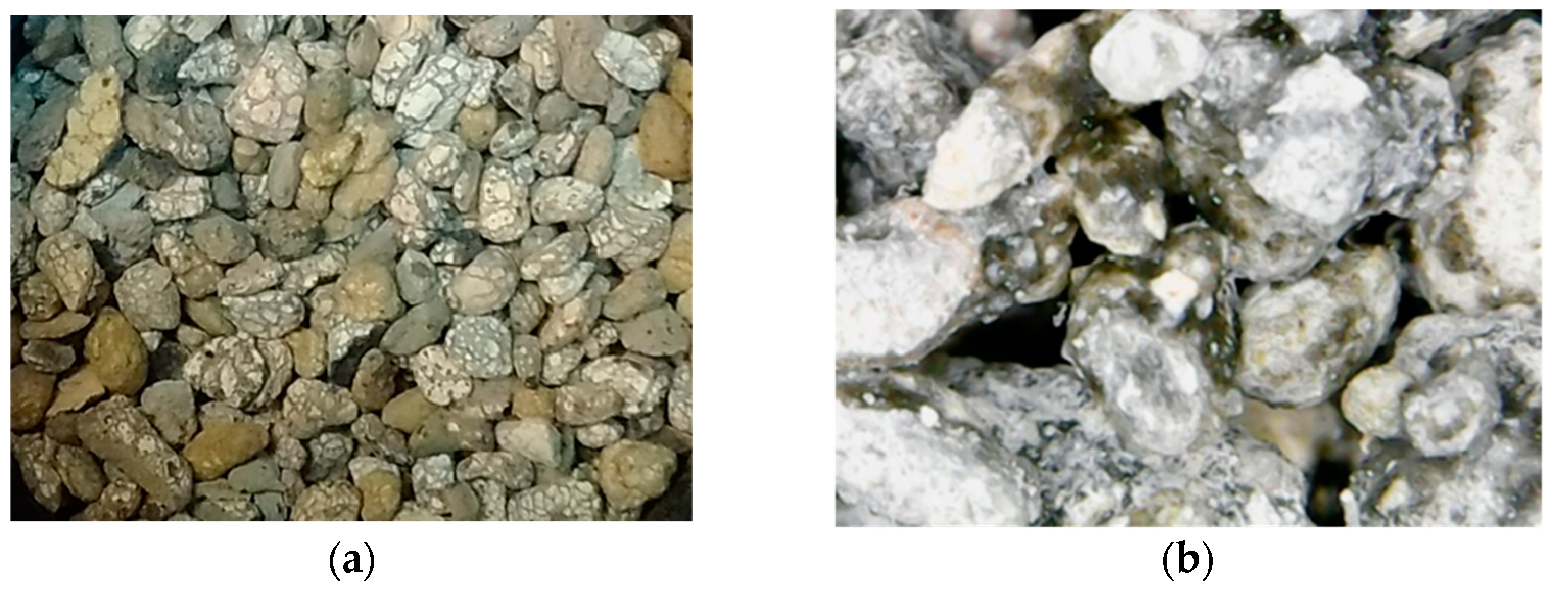
Due to the relevance of using an absorbing layer, in this work, porous materials were studied to be incorporated on the face of the acoustic barrier exposed to railway noise. Excellent qualities, such as high workability, low density, and sufficient mechanical resistance, may be found in porous concrete with light aggregates and an adequate amount of air. It can also be used to make architectural elements with appropriate acoustic and thermal behavior [15]. A porous material is made up of a solid structure containing cavities, tunnels or pores filled with air, and the interaction of sound waves with these two phases causes sound energy dissipation [13,16]. Consequently, a possible approach to study sound propagation in a rigid-frame porous material is to model the fluid-filled medium as a homogeneous fluid with complex, frequency-dependent characteristic impedance and propagation constant.
Several experimental and theoretical approaches may be used to study porous materials. As suggested in ISO 10534-2 [17], using an impedance tube to evaluate the sound absorption coefficient with normal incidence is a low-cost and simple approach that yields relevant information. However, it has certain drawbacks because different sound incidence angles are typically present in real-world situations. The values for the material’s surface impedance are also provided by this approach, though. The method suggested by ISO 354 [18] may be used to experimentally estimate the sample’s sound absorption coefficient under diffuse field conditions. This experimental methodology is more onerous than the previous one, but presents the benefit of considering different sound incidence angles and uses a larger sample, which is a scenario closer to real application.
Theoretical methods have been proposed by some authors in order to derive values of sound absorption in diffuse field conditions based on values determined with normal incidence approaches [19]. The transition from the sound absorption coefficient with normal incidence, obtained using an impedance tube, to the diffuse field coefficient can be made with London’s equations [6,19]. In these conditions, the medium has to be considered infinite and the propagation inside the medium is locally reactive. To describe the absorbing behavior of the porous materials under study, fluid-equivalent models, taking into account the complex bulk modulus and fluid-equivalent density, have been proposed [14,20,21,22,23,24].
Works related to the sound-absorption properties of granular materials have been developed by Asdrubali and Horoshenkov [25], showing some expected values of the macroscopic parameters for materials incorporating expanded clay. Vasina et al. [26] and Carbajo et al. [27] also presented works with granular materials for sound absorption purposes. These are of particular interest, revealing some estimated values of the relevant properties for expanded clay-based materials. Porous concrete, like most porous materials, is composed of pores of varying shapes and sizes. Although variation in the shape of the pores is less important, the statistical parameters of the pore size distribution can have a considerable effect on the acoustic properties of the porous media [28]. Based on these previous studies, it becomes possible to predict the behavior of porous materials through theoretical and numerical models [22,28,29].
In this study, the Horoshenkov–Swift [20] model has been used, since it is quite adequate to model granular materials. In that model, the porous materials are represented as equivalent fluids [23]. Four parameters—air-flow resistivity, tortuosity, open porosity, and the standard deviation of the pore size—are used in this model to describe how the porous material behaves in terms of sound absorption.
Aside from modeling the acoustic behavior of the surface material of the barriers, it is of utmost importance to assess the global behavior of the acoustic barrier, in particular in what concerns the reduction in the environmental noise it provides for protected receivers. This topic has been addressed by numerous authors, using different methods. Indeed, engineering calculation methods, such as those proposed in the CNOSSOS-EU methodology or in the ISO 9613-2 [30] can be used to estimate the insertion loss provided by specific noise barrier solutions, also taking into account the environmental setting in which it is implemented. More advanced methods, based on the use of numerical methods that solve the wave equation in the time or frequency domains, can also be used to have a more detailed and theoretically accurate view of the effect of these devices. Several works make use of advanced numerical methods, such as the Boundary Element Method (BEM), including some reference works, such as [31], and many publications by the co-authors of the present paper [32,33,34]. Indeed, the BEM has proven to be an excellent tool to simulate the scattering of waves around a noise barrier, as it accurately accounts for geometrical details of the structure and allows including different effects, such as the sound absorption of its surface. For example, in [34], noise barriers with complex surface geometries are analyzed, including strong diffusion effects generated by a so-called “s-QRD” barrier profile. In a more recent paper, meshless methods, such as the Method of Fundamental Solutions [35], are also used with success.
The present paper intends to contribute to the body of knowledge on this topic by analyzing noise barriers with absorbing materials, both from a point of view of the material itself and from the point of view of their simulation, not only as an obstacle, but also including the effect of the material. The specific case of barriers with an absorbing layer of porous concrete including expanded clay is addressed. A methodology is here first developed to derive adequate parameters to model this material using the equivalent fluid Horoshenkhov–Swift model. This strategy is based on the measurement of the relevant macroscopic parameters in the laboratory, together with the sound absorption curve (using an impedance tube), and then, using an optimization algorithm to adjust the macroscopic parameter values in order to minimize the difference between the result obtained using the theoretical model and the experimental measurement. Although the strategy is inspired by other works, such as [36], here, the initial approximation is derived from the material characterization and not completely obtained by inversion; the optimization process only allows relatively small variations of those parameters (up to 10%) to allow a better match between the measured and estimated sound absorptions. Normal incidence sound absorption results are then used to predict the diffuse field behavior of the material using different approaches, and results are compared with measurements performed following ISO 354 [18]. An important question that arises is related to the sensitivity of the numerical and engineering models used in environmental noise simulation with respect to the sound absorption values ascribed to the noise barrier surface. Indeed, results obtained in a reverberant chamber can exhibit significant differences from those derived from normal incidence conditions by applying simple expressions such as the classical ones proposed by London [19], but the relevance of these differences in simulation models is not really known. Here, a study considering both the CNOSSOS-EU calculation method and BEM model are used to address this topic. Since this study has been developed within the scope of the development of railway noise barrier solutions, two types of barriers are analyzed, a classical noise barrier, positioned at a significant distance from the railway track, and a low-height barrier, positioned very close to the track and subsequently to the noise source. Two different shapes are analyzed for each case, corresponding to a vertical barrier and to an L-shaped barrier. For all situations, both purely reflective and absorbing barriers are simulated.
The paper is organized as follows: first, the materials and methods are presented, including a description of the used materials and of the test methods adopted for its characterization; results of this characterization are then presented and discussed, considering normal incidence conditions; this is followed by an estimation of the absorption of the tested materials considering diffuse field conditions, using different models and comparing with values measured in a reverberant chamber; finally, numerical simulations considering the application of the porous concrete in low-height and traditional noise barriers are performed.

2. Materials and Methods

Following the scope described in the introduction, it is important to clearly define the materials used in the context of this study and the experimental, theoretical and numerical methods used in their characterization, modeling and simulation. First, the porous concrete used in all the analyses is described, followed by a brief description of the experimental methods used in its characterization, both from a physical and acoustic point of view. The theoretical models used in the detailed material analysis are then presented, together with the methods adopted to predict the diffuse-field acoustic behavior under normal incidence results. Then, an overview of the methods used to simulate the noise barriers is also given.

2.1. Porous Concrete Specimens

Expanded clay with a size range of 0–4 mm was used as aggregate material (Figure 1) for the production of the specimens analyzed in this work. Granulometric analysis was performed to characterize this granular material in terms of the distribution of its particles as a function of its size. The grain size distribution, in accordance with EN 933-1 [37], is presented in Figure 2.
Having in mind the purpose of performing acoustic measurements in an impedance tube, several concrete-based mixtures were prepared by incorporating expanded clay (Figure 3). The cylindrical test specimens had an approximate diameter of 10 cm, and two sets with thicknesses of 4 and 8 cm were manufactured.
The test specimens with expanded clay were prepared for 3 Aggregate/Cement ratios (A/C), with a total of 6 samples per porous concrete mixture. Of those, three samples were made with a thickness of 4 cm, and the remaining three were prepared with a thickness of 8 cm (see Table 1).
For the tests performed in the reverberant room in diffuse field conditions, following ISO 354 [18], an additional porous concrete specimen was produced, with an approximate total area of 10 m2 (Figure 4). In this case, the porous layer observable in Figure 4 had a thickness of eight centimeters, was placed over a concrete structural layer and mounted directly against the floor of the reverberation room with the perimeter edges covered by a reflective rigid frame (type A mounting, described in Annex B of ISO 354 [18]).

2.2. Experimental Methods

The adopted experimental and theoretical methodologies are presented below. Firstly, the macroscopic parameters of the material were experimentally determined, making the application of a fluid-equivalent material model possible to estimate sound absorption under normal incidence conditions. Then, the sound absorption coefficient was also determined under normal incidence conditions using an impedance tube, and for diffuse field conditions in a reverberant room.

2.2.1. Macroscopic Parameters

To make use of theoretical material models that allow simulating the acoustic behavior of granular porous materials, it becomes necessary to experimentally obtain a number of macroscopic parameters that characterize the porous material itself. For the purpose of this work, the required parameters were the porosity, the tortuosity, the airflow resistivity, and the standard deviation of the average pore size of the porous concrete samples.
The porosity of the test specimens was determined, after drying the samples to constant mass (at 70 ± 5 °C), by weighing the test specimens on a hydrostatic balance and immediately after removing the excess water with a damp cloth. Porosity was determined experimentally using the water-saturation method (based on [38]) and this parameter is given by:
ϕ = V f / V t
in which: V f = ( M sat M d r y ) / ρ water is the void volume of the porous concrete sample, and V t is the sample total volume.
For the determination of the samples’ tortuosity, a laboratory experiment, based on the electrical conductivity of the sample and described in the work developed by Gerges and Balvedi [39] (see Figure 5a), was implemented and used. In this technique, the test specimen is mounted in a PVC tube that is closed by two electrodes. Next, the tube is filled with a conductive liquid (in this study, salty water) and a power supply generates an electric field between the two electrodes at the ends. Electrical potential differences in the water and sample make it possible to determine the tortuosity of the porous concrete sample.
Following this methodology, tortuosity is then given by the following expression:
α = ϕ σ a σ f
where: ϕ is the sample porosity; σ a is the electrical resistivity of the sample saturated with the fluid, and σ f is the electrical resistivity of the fluid.
Using the method described in ISO 9053-2 [40], the airflow resistance and airflow resistivity of the porous concrete samples were determined. This procedure is based on the alternating airflow method, a condition of paramount relevance to ascertain the alternating component of the pressure in the test volume. The following equation defines the airflow resistivity:
σ = R s d
with Rs being the specific airflow resistance, of the test specimen, in Pa·s/m, and d being the thickness of the test specimen in the direction of flow (in m). Figure 5b shows the experimental apparatus used.
The only parameter that has not been obtained by means of laboratory measurements was the standard deviation of the average pore size, σp. Indeed, this is not a simple parameter to estimate in the laboratory, and the authors opted to adopt average values based on the work of Pereira et al. [36].

2.2.2. Measurement of the Sound Absorption Coefficient

To obtain the sound absorption coefficient under normal incidence conditions, laboratory tests were performed on a circular impedance tube with 100 mm internal diameter (Figure 6). The test methodology is described in ISO 10534-2 [17], which is based on the transfer function between two microphones.
The impedance tube used has a cut-off frequency of about 1600 Hz. The sound pressure was measured using two G.R.A.S. Sound and Vibration (Denmark) 46 AE 1/2″ CCP Free Field microphones, a NI USB-4431 dynamic signal acquisition (DSA) device, from National Instruments (USA), connected to a PC laptop and the registered pressure data has been recorded and processed in MATLAB 2016 implemented codes. A random excitation, provided by a loudspeaker in one end of the impedance tube, was generated from the NI USB-4431 DSA.
The ratio between the reflected pressure (pr) and the incident pressure (pi) is the reflection factor that is given by:
r = p r p i .
On the other hand, the sound absorption coefficient can be achieved with the following expression:
α = 1 | r | 2 .
where r is the reflection coefficient. This experimental test also provides an important parameter that characterizes the acoustic absorbing material, the surface impedance, given by:
Z s f = ρ 0 c 0 ( 1 + r ) ( 1 r ) .
where Z 0 = ρ 0 c 0 is the characteristic air impedance.
To evaluate the sound absorption in diffuse field conditions, experimental tests were performed on a reverberant room. This test methodology is proposed in ISO 354 [18]. The diffuse incidence absorption coefficient measurement procedure consists of making reverberation time (RT) measurements of the reverberant room under two distinct conditions: firstly, with the reverberant room empty and, afterwards, with the sample to be characterized placed directly over the floor of the reverberation room, with the perimeter edges of the test specimen sealed with a reflective frame of gypsum boards and reflective adhesive tape sealing the joints along the perimeter (see Figure 7). In accordance with the above-mentioned standard, based on Sabine’s formula, the equivalent absorption area of the porous concrete sample can be achieved with:
A T = A 2 A 1 = 55.3 V ( 1 c 2 R T 2 1 c 1 R T 1 ) 4 V ( m 2 m 1 ) ,
in which V corresponds to the volume of the empty reverberant room, c 1 corresponds to the propagation speed of sound in air at temperature t 1 with the empty room, m 1 corresponds to the attenuation coefficient due to the presence of air with the empty room, R T 1 corresponds to the reverberation time of the empty room, and c 2 corresponds to the sound propagation velocity in the air at temperature t 2 with the sample placed in the room, m 2 corresponds to the attenuation coefficient due to the presence of air with the sample in the room, and R T 2 corresponds to the reverberation time with the sample in the reverberant room. The sound pressure was measured using two G.R.A.S. Sound and Vibration 46 AE 1/2″ CCP Free Field microphones, a Symphonie acquisition system, from 01 dB, with dBBati32 controlling software.

2.3. Material Modeling

2.3.1. Horoshenkhov–Swift Model

For porous concrete, the Horoshenkov and Swift [20] model for granular porous materials was applied by taking into account porosity, ϕ, airflow resistivity, σ, tortuosity, α , and the standard deviation of the pore size, and σp, as material parameters. The first three have been calculated empirically [34,35,36,37] and by using an inverse technique approach (see below, in Table 2, experimental and adjusted values). The last parameter, σp, however, was only determined theoretically. These authors suggest to calculate the volumetric density and compressibility module of the porous material using the following equations:
ρ = α ϕ ( ρ 0 j ϕ σ ω α F ˜ ( ω ) ) ,
C = ϕ γ P 0   ( γ ρ 0 ( γ 1 ) ρ 0 j σ ϕ ω α N p r F ˜ ( N p r ω ) ) ,
in which ω corresponds to the angular frequency, γ to the ratio of specific heats, P0 to the atmospheric pressure and Npr is the Prandtl number, and F ˜ ( ω ) is the viscosity correction function, that can be presented in the form of a Padé approximation as:
F ˜ ( ω ) = 1 + a 1 ϵ + a 2 ϵ 2 1 + b 1 ϵ ,
where a 1   = θ 1 / θ 2 , a 2 = θ 1 and b 1 = a 1 . Assuming that the geometry of the pores is circular, in a simplified way, comes the following form factors: θ 1 = 4 3 e 4 ξ 1 , θ 2 = e 3 ξ / 2 2 , where ξ = ( σ p   ln ( 2 ) ) 2 and ϵ = j ω ρ 0 α / ( σ ϕ ) .
In order to theoretically estimate the macroscopic parameters and evaluate a new sound absorption curve of the porous material, an inverse technique based on a genetic algorithm was also applied. This methodology is based on the difference between the theoretical sound absorption coefficient results, obtained with the Horoshenkov– Swift model, and the experimental sound absorption coefficient data. Each macroscopic parameter was given an initial estimation (based on the experimental findings) as well as lower and upper boundary limits in order to be used with this inversion procedure. A variation limit of 10% was imposed. This procedure makes sure the values remain within acceptable bounds. The objective function (11) that follows is then minimized:
F u = i = 1 n f | α s a α s e | 2 ,
In this equation, nf is the number of discrete frequencies analyzed, α s a is the absorption coefficient results determined by the Horoshenkov– Swift model and α s e corresponds to the experimental absorption coefficient data.
Figure 8 shows a flowchart of the inversion methodology used to determine the macroscopic parameters.

2.3.2. Prediction of Diffuse Field Sound Absorption

The so-called first and second London equations [19] are theoretical models that employ some simplifications to transform the results obtained in terms of the sound absorption coefficient for normal incidence to diffuse field coefficients. They are presented in the following equations:
α b = 8 [ 1 1 α n 1 + 1 α n ] 2 [ ( 2 1 1 α n ) 1 1 α n 2 + 2 l n ( 1 1 α n 2 ) ] ,
α s = 4 [ 1 1 α n 1 + 1 α n ] [ l n ( 2 1 1 α n ) 1 + 1 α n 2 ] ,
where α n is the experimental sound absorption coefficient under normal incidence conditions.

2.4. Noise Barier Modelling

In this work, an attempt was made to understand whether the calculation and simulation models allow taking into account, adequately, the presence of different types of noise barriers, including reflective and absorbing barriers, as well as traditional (tall) and low-height barriers (with about 1.5 m). For barriers with an absorbing surface, the properties of the porous concrete material with expanded clay analyzed before, and with a thickness of 0.08 m [41,42], were considered. Different scenarios were simulated, considering a simple reference configuration without any acoustic barriers, and then the same scenario with the presence of acoustic barriers with heights of 1.5 m and 4 m. The distance between the barriers and the noise source varies according to their height, with the low-height barriers being positioned 2.83 m from the source, and the traditional tall barriers 7.5 m from it. These distances were defined assuming a possible railway track as the emitting source, and so these distances, for the first case, were based on a minimum allowable distance between the track and the barrier (maintaining the safety conditions), and for the second case, they were defined based on common distances adopted in the railway infrastructures in Portugal [43]. Two different barrier shapes were considered, one of them vertical and the other a L-shaped barriers, and cases with and without an absorbing layer were tested. Figure 9 presents a schematic representation of these configurations.
Numerical simulations were performed using two methodologies, the first one based on a commonly used environmental noise simulation software (CadnaA), implementing the CNOSSOS-EU methodology [5], and the second adopted a Boundary Element Method (BEM) in the frequency domain [32,33,34], developed and implemented in MATLAB.
For the first methodology, the emitting sound source was assumed to be a train, and the sound powers were corresponding to a BR 1016 train, with a constant speed of about 80.47 km/h (50 mph) being used for the simulation. Horizontal meshes were made of receivers placed at heights of 1.5 m and 4 m, spaced 1 m apart, and a vertical mesh, transverse to the track, with receivers equally spaced 1 m apart was considered. The source is located at 0.5 m height and the absorption coefficient of the soil was assumed to be 0.3 [5].
For the BEM, the calculation is based on solving the boundary integral equation:
C ( ξ ) p ( ξ ) = i ρ ω Γ G ( ξ , X ) v n ( X ) d Γ Γ G ( ξ , X ) n p ( X ) d Γ + k = 1 N S Q k G ( ξ k f , ξ )
where Γ represents the boundary surface, ρ the propagation medium density (1.22 kg/m3 in the case of air), G ( ξ k f , ξ ) the incident field generated by a source located at ξ k f , and p ( X ) and v n ( X ) represent the unknown pressure and velocity of the particle, respectively. C ( ξ ) depends on the boundary geometry and takes the value ½ for a smooth boundary.
The sound absorption of the different surfaces is imposed through a Robin-type boundary condition, in which the surface acoustic impedance is prescribed as Z = ρ c ( 1 + 1 α ) / ( 1 1 α ) , α being the sound absorption coefficient derived from diffuse field conditions. To allow assigning the necessary impedance conditions to the soil, it is also discretized using boundary elements along a 25 m extension (from x = −5 m to x = 20 m). In the simulated cases, it was decided to locate the sound source at the height of 0.5 m, following the same strategy indicated in the previously described CNOSSOS-EU model.
The insertion loss (IL) parameter has been used to characterize the acoustic performance of the barrier, obtained through the equation:
I L = S P L s b S P L c b = 20   l o g   ( | P s b | | P c b | )
where SPLsb is the sound pressure level without a sound barrier, SPLcb is the sound pressure level with a sound barrier, Pcb is the sound pressure with a sound barrier and Psb is the sound pressure without the sound barrier.

3. Results and Discussion

In this section, a summary of the results obtained in the development of the work and their respective analysis and discussion are addressed. First, results are presented and analyzed regarding the acoustic and non-acoustic characterization of the absorbing porous material, including the macroscopic parameters, sound-absorption coefficient under normal incidence, and diffuse field conditions, calculated through different methodologies. Next, the results and respective discussion are presented relative to the effect of incorporating the studied porous concrete material in different noise barriers.

3.1. Material Parameters and Acoustic Behavior

Table 2 shows the results obtained for the experimental and corrected macroscopic parameters for each Aggregate/Cement sample shown in Table 1, with a thickness of 8 cm. These parameters were determined as the average of the experimental test values of three samples for each Aggregate/Cement ratio.
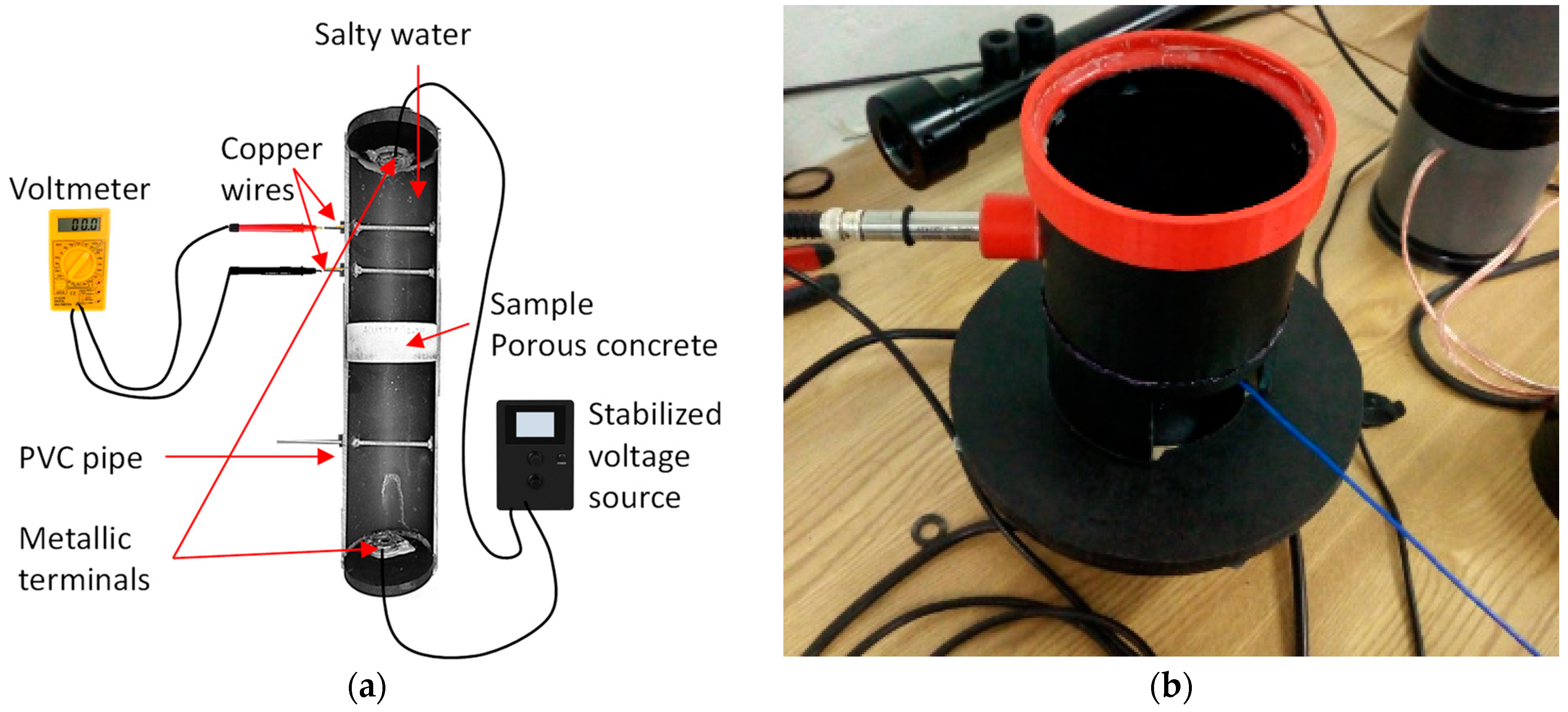
Observing, first, the experimental values measured in the laboratory, it can be seen that the measured values of the tortuosity, porosity, and airflow resistivity are relatively similar for the three sets of samples analyzed, with no significant variations when the Aggregate/Cement ratio is changed. This result indicates that there is no advantage, concerning acoustical absorption, in using higher cement quantities in the production of this type of material, and using the minimum that ensures sufficient mechanical stability and durability is an adequate choice. Although this was expected, it is also interesting to note that, if improved mechanical properties are required, for a specific application, the moderate increase in the cement quantity does not degrade the acoustical absorption properties.
The adjustment procedure proposed above has then been used to fine-tune the macroscopic parameters, in order to obtain a better match of the sound absorption estimated using the Horoshenkhov–Swift model with the one measured using the impedance tube. One should note that only small variations were allowed, with a maximum of 10%. Observing the adjusted values of the macroscopic parameters, it is possible to note that the larger changes occur in the tortuosity values, which reached almost 10% in two of the sets. It should be mentioned that the test method used, based on the electrical conductivity of the sample, can pose some challenges in laboratory implementation and can present variations from specimen to specimen. As for the porosity and airflow resistivity, only the sample type AE 5.18 required more significant adjustments, while the remaining only required minor adjustments. The same occurred for the average pore size standard deviation, although in this case, the initial value was just fixed based on the literature.
The theoretical and experimental curves for the sound absorption coefficient with incident plane waves are displayed in Figure 10. The experimental outcomes were attained in compliance with the ISO 10534-2 [17]. The theoretical curves were achieved with the model proposed by Horoshenkov and Swift, where experimental macroscopic parameters (PMe) and corrected macroscopic parameters (PMc) were used. The curves exhibit the typical behavior of a porous concrete material, with a peak–valley structure, in which a significant peak occurs around 650 Hz. This position of the sound absorption peak is mainly related to the thickness of the sample, as other tests with different thicknesses have revealed (presented later in this section).
It can be seen that the experimental results were well-fitted by both theoretical curves, even before the adjustments were performed. However, it can also be seen that the adjustment procedure allowed for a better final agreement between the experimental and theoretically derived curves, as expected. This is particularly evident in the case of the AE 5.18 sample, which, even after the adjustment, still revealed some discrepancies.
Despite having distinct Aggregate/Cement ratios, the samples exhibit relatively similar behaviors, since the differences between them are negligible. Between 400 and 1000 Hz, significant sound absorption can be observed for all cases. It can also be seen that the sound absorption curve shifts very slightly to lower frequencies when higher cement contents are considered. As the cement composition increases, the sample’s density rises as well, resulting in narrower pores and channels, hence altering several macroscopic factors that affect the samples’ acoustic behavior.
An additional cross-validation test was performed, which consisted in calculating the sound absorption curve under normal incidence considering 4 cm thick specimens, and comparing it with the same parameter measured in an impedance tube. This comparison provides interesting information, since it is performed with specimens that have not yet been used in the previous calculations, and thus it is truly independent of the remaining procedure. Figure 11 presents the corresponding results. It is clear, as expected and mentioned before, that the sound absorption peak is shifted to higher frequencies, although still maintaining a very high value (almost 1.0). The theoretical curves from the Horoshenkov–Swift model seem to predict the occurrence of the peak at slightly higher frequency values, which may be due to different factors, such as the variability of the porous concrete material itself between samples of 8 cm and 4 cm thickness during the production stage of the different specimens.

3.2. Sound Absorption Coefficient under Diffuse Incidence—Experimental vs. London’s Equations

In Figure 12 and Figure 13, the experimental and theoretical sound-absorption coefficient curves in diffuse field conditions are presented for the mixture AE 5.18. The theoretical simulation and the experimental results were obtained for all scenarios using a thickness of 8 cm.
Results for normal incident waves and for a diffuse field show considerably distinct behaviors when comparing the sound absorption curves obtained for both scenarios. As anticipated, the diffuse field curves exhibit a broader frequency range where significant sound absorption is obtained, clearly demonstrating the action of refracted sound waves inside the porous concrete material volume.
When comparing the various methods for estimating diffuse field sound absorption, London’s Equation 1 (London 1 exp.data 008 and London 1 HS PMc 008) appears to fit the experimental curve more closely, particularly the one produced using the Horoshenkov–Swift model and the adjusted macroscopic properties of the examined material. Although it predicts greater values at lower frequencies and smaller absorption values in the mid-frequency region, the second London equation also yields findings that are comparable. It should be emphasized that the predicted diffuse field absorption using London’s equations is merely a rough estimate and should not be used for anything other than the analysis of locally reacting materials. Since the tested solution, in this scope, is obviously bulk-reacting, considerable variations take place. Additionally, the diffuse field laboratory test was performed on a finite 3 × 3 m2 panel, although all equations apply to infinite panels, thus resulting in different behavior of the whole solution (see [36]).
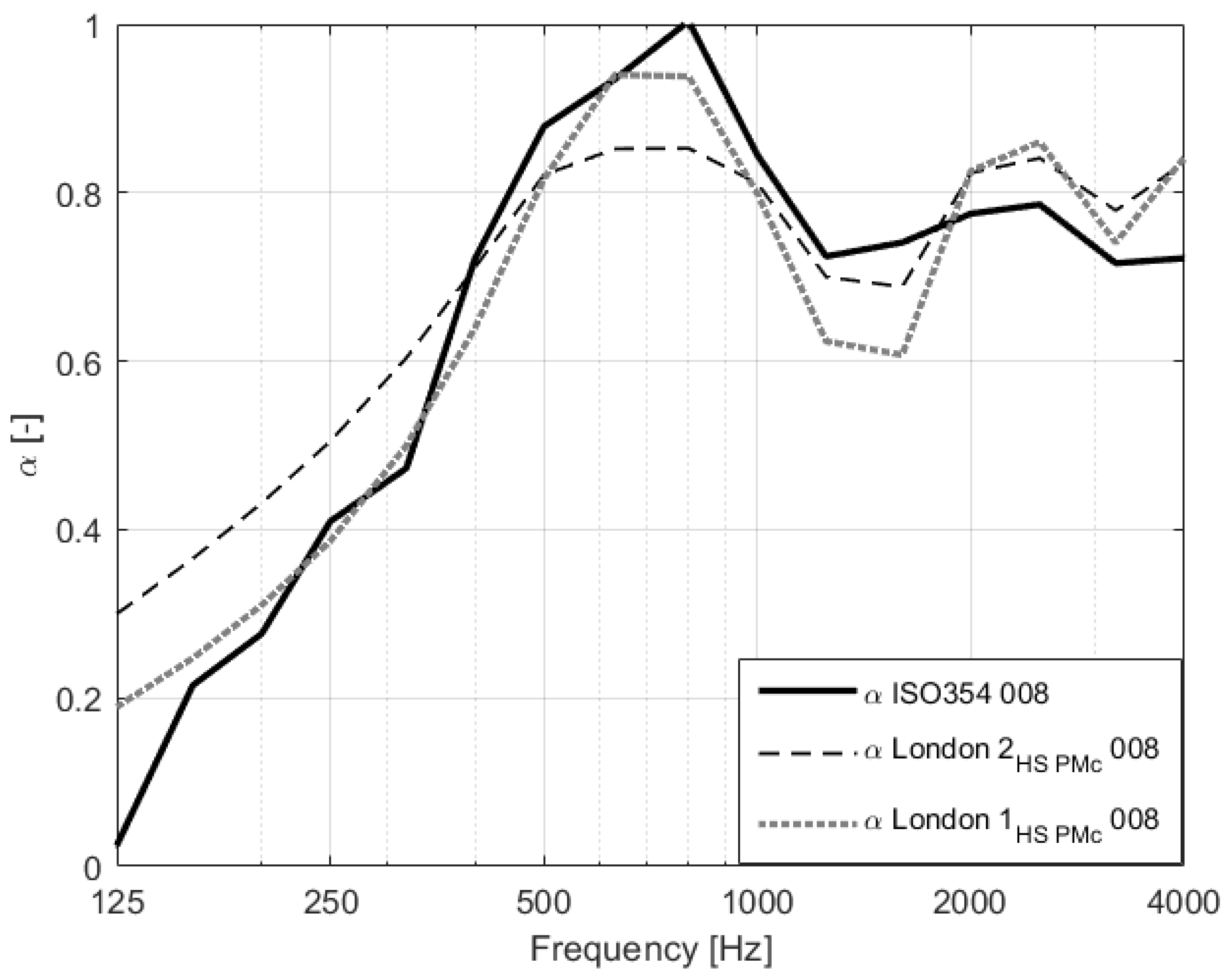
Figure 13 shows a final plot comparing the observed sound absorption derived from the reverberant room test together with the two London models, considering bands of one-third of an octave and the entire frequency range between 125 Hz and 4000 Hz. These curves demonstrate that the two simple models provide a good estimation of the trend of the sound absorption curve, albeit with some apparent inconsistencies and oscillations. The predictions based on the Horoshenkov–Swift theoretical model along with the London models appear to relate well with the experimental curve, even in the higher frequency range beyond 2000 Hz (which was not measured in the impedance tube). Nevertheless, the match is clearly not perfect and some deviations can be observed.

3.3. Noise Barrier Simulation

The material analyzed above has been incorporated into different numerical models, as described in Section 2. Initially, a first set of simulations was performed using CadnaA prediction software, in order to estimate the change in the noise levels on the source side of the barrier using the CNOSSOS-EU methodology. Receivers were placed 0.25 m from the barrier’s surface so as to correctly assess the changes in the noise levels introduced by its presence. The simulated scenario was also described in Section 2 and considers a passing train, with the noise emission spectrum calculated from CNOSSOS-EU. Flat barriers were used in this first comparison, considering both a reflective noise barrier (designated in the plots as α 0.01) and three variants of the barrier with an absorbing layer, identified as ISO 354, London 1, and London 2. The sound absorption curves of the absorbing layers were obtained, one experimentally (ISO 354) and the other two through the London equations (London 1 and London 2), as depicted in Figure 13. It can be observed that the theoretical curves obtained with both London’s equations are very close to the ones computed from experimental sound absorption values under diffuse conditions. On the other hand, as expected, it appears that next to the absorbing layer of the noise barrier, there are lower sound pressure levels compared to a reflective barrier. Clearly, the approximation given by London’s equations is sufficient to allow their use in environmental noise prediction models without significant loss of accuracy. The influence of the absorbing material is particularly noticeable in the mid-high and high frequencies (see Figure 14), where the higher sound absorption values are registered. The same type of behaviour is registered both for the 4 m and 1.5 m tall barriers, although with different SPL levels values due to the different distances from the source. It should be noted that on the source side of the barrier, it is always expected to observe an increase in the sound pressure levels with respect to a reference situation without any noise barrier (not shown), due to the constructive combination of the incident wave with the first reflection from the surface.
One of the main objectives of this paper was to compare, for different scenarios, the results obtained with the CNOSSOS-EU methodology with those given by a detailed numerical code solving the frequency domain acoustic wave equation with the BEM. The physical principles that form the basis of each calculation method are quite different, with the first one being energy-based, without accounting for phase change during propagation, while for the second the complete physical phenomenon is being taken into account in the modelling process. The chosen parameter for comparison purposes of the acoustic performance was the Insertion Loss (IL). Flat (α 0.01, ISO 354, London 1, London 2, and CadnaA) and L-shaped (α 0.01 L, ISO 354 L, London 1 L, London 2 L, and CadnaA L) noise barriers were used in this evaluation. The studied configurations have been schematically described in Figure 9, and include reflective barriers (α 0.01) and barriers with an absorbing layer on the exposed side to the noise source (ISO 354, London 1 and London 2). The sound-absorption curves of the absorbing layers were obtained experimentally (ISO 354) and through the London equations (London 1 and London 2).
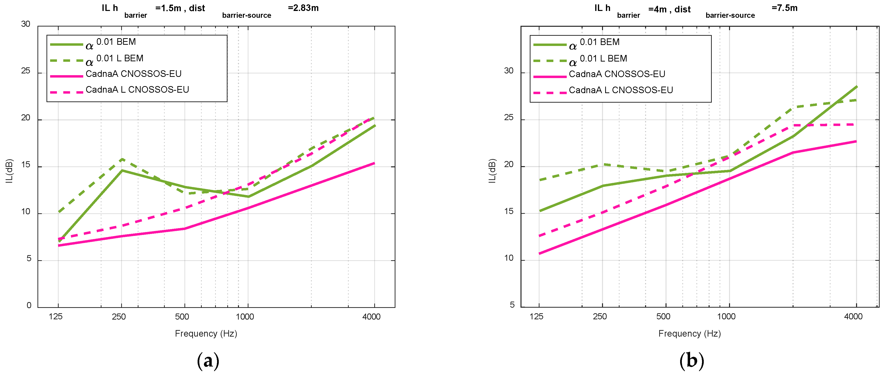
In Figure 15a,b, results calculated by both methodologies are shown considering a rigid reflective barrier. Both L-shaped and vertical noise barriers were analysed, both for the low-height and tall barriers. It is clear that the curves of IL obtained with CNOSSOS-EU exhibit lower IL values, in particular at lower frequencies, and they tend to have a more regular behaviour throughout the analysed frequency domain. The fact that this method is mostly based on following the path and energy of sound waves, without accounting for the oscillatory character of the wave propagation may help in justifying this result. The BEM results exhibit a less regular behaviour, due to the oscillatory character that is accounted for in this numerical methodology. The two methods seem to predict more similar IL values at higher frequencies. As expected, the L-shaped cantilevered barrier returns higher insertion loss values than the flat barrier since the top of the barrier limits the diffractions of the waves that pass to the other side of the barrier. However, for the BEM calculation and for the low-height barrier, this difference is quite small.
In Figure 16a,b, the influence of the porous material on the insertion loss curve is observed. This influence is visible mainly for the mid-high frequencies, for which the studied material exhibits higher sound absorption values. In that range, noise barriers with an absorbing layer have somewhat better acoustic performance (higher IL values) than reflective barriers. However, the change registered in the vertical barrier results, due to the introduction of sound absorption, is very small and never exceeds 1 dB. In that case, since the sound absorption is located on the source side it affects mostly the reflected field, and very little changes occur behind the noise barrier. For an L-shaped barrier with sound absorption on the inner part, no changes are visible, and thus this case is not represented. In this respect, it should be noted that all the curves in this plot have been obtained with BEM. Indeed, when the sound absorption is introduced in the CNOSSOS-EU model of CadnaA, no differences were registered either in the L-shaped or in the vertical barriers with respect to the case of the reflective barrier; for those cases, since the sound absorption is located only on the source side of the barrier, only the sound levels on that side seem to be affected and no changes are registered behind the noise barrier.
The described behavior changes considerably if the sound-absorbing material is also introduced on the top of the L-shaped cantilevered noise barrier, whose numerical result calculated with the BEM is also depicted in Figure 16. Clearly, the presence of the sound-absorbing porous material seems to have a strong influence on the diffraction phenomenon that occurs in this barrier, providing an additional attenuation at high frequencies. This increase can be of up to 5 dB at the higher frequencies, which is quite a remarkable improvement but one that still requires experimental validation. At this point, it is worth mentioning that both the low-height and the more traditional tall vertical barrier provide significant noise protection, which can go up to 25 dB, for the first, and 32 dB, for the second types of noise mitigation devices. Indeed, this result also indicates that the smaller noise barriers placed closer to the source can be a viable alternative to the conventional taller ones whenever space restrictions, aesthetics or visual impact effects are relevant.
Finally, Figure 17 compares the results obtained with the BEM considering the sound absorption coefficients derived from the experimental test (ISO 354) and from the application of London 1 and 2 equations (Equations (15) and (16)). It is interesting to underline that differences no greater than 1.5 dB (for the L-shaped barrier, with sound absorption on the top surface) are registered in this comparison, throughout the frequency range. In general, the three curves follow very similar trends, for both noise barrier types, which indicates, once more, that a sufficient level of accuracy can be obtained with a simple acoustic prediction performed based on London’s equations.

4. Conclusions

The main objective of this work was to assess the efficiency of acoustic barriers incorporating a sound-absorbing material made of porous concrete in the railway context, defining adequate material models and testing different calculation methodologies.
For the definition of the material itself, the effect of the Aggregate/Cement ratio and thickness of the absorbing porous layer on the solution’s acoustic behavior was first studied, and the obtained results indicated that, within moderate values of the cement content, the open porosity of the material is still effective. A proposal of an inversion technique to obtain macroscopic parameters required by the acoustic material model was presented, with an optimization algorithm which uses the first approximation macroscopic parameters measured in the laboratory with good results on several mixtures; cross-validation with samples with different thicknesses was performed, with acceptable results. Diffuse field sound-absorption curves computed from normal incidence coefficients using simple expressions proposed by London allowed to obtain good correlation with large specimens measured in a reverberant room under diffuse field conditions.
Several scenarios of noise barriers were simulated, taking into account different barrier shapes and with and without absorbing porous surfaces. Significant differences were found between the two calculation methods used here, namely the CNOSSOS-EU and BEM models in the frequency domain, with the first providing usually lower predictions of the insertion loss acoustic performance. The use of the BEM numerical method allowed for a more detailed analysis of the effect of acoustically absorbing materials. A relevant observation was related to the inclusion of absorbing material on the top surface of L-shaped cantilevered barriers, which seems to allow for a significant additional insertion loss acoustic performance of these noise barriers.

Author Contributions

Conceptualization, P.A.-M. and L.G.; Methodology, P.A.-M. and L.G.; Software, L.S., D.M.-G. and L.G.; Formal analysis, L.S., D.M.-G., J.M.B.-M., P.A.-M. and L.G.; Investigation, L.S., L.P. and D.R.; Data curation, L.S. and L.P.; Writing—original draft preparation, L.S., L.P. and L.G.; Writing—review and editing, D.R., D.M.-G., J.M.B.-M. and P.A.-M.; Funding Acquisition, P.A.-M. and L.G. All authors have read and agreed to the published version of the manuscript.

Funding

This research was partially funded by FCT—Fundação para a Ciência e a Tecnologia, I.P., by Base Funding (UIDB/04029/2020) and Programmatic Funding (UIDP/04029/2020) of the research unit “Institute for Sustainability and Innovation in Structural Engineering—ISISE”, and under the Associate Laboratory Advanced Production and Intelligent Systems ARISE under reference LA/P/0112/2020. This work was also funded by FEDER funds through the COMPETE 2020, Portugal 2020, under the projects POCI-01-0247-FEDER-033990 (iNBrail) and POCI-01-0247-FEDER-046111 (FERROVIA 4.0), by national funds (PIDDAC) through FCT/MCTES under the project PTDC/ECI-EGC/3352/2021 (IntRAIL).

Conflicts of Interest

The authors declare no conflict of interest.

References

  1. World Health Organization (WHO). Health Topics. Environment and Health. Noise, WHO Regional Office for Europe, Copenhagen (Denmark). 2021. Available online: https://www.euro.who.int/en/health-topics/environment-and-health/noise/noise (accessed on 1 September 2022).
  2. Ibrahim, R.A. Recent advances in nonlinear passive vibration isolators. J. Sound Vib. 2008, 314, 371–452. [Google Scholar] [CrossRef]
  3. Zhang, X.; Liu, R.; Cao, Z.; Wang, X.; Li, X. Acoustic performance of a semi-closed noise barrier installed on a high-speed railway bridge: Measurement and analysis considering actual service conditions. Measurement 2019, 138, 386–399. [Google Scholar] [CrossRef]
  4. Liu, J.; Guo, H.; Wang, T. A review of acoustic metamaterials and phononic crystals. Crystals 2020, 10, 305. [Google Scholar] [CrossRef] [Green Version]
  5. Kephalopoulos, S.; Paviotti, M.; Anfosso-Lédée, F. Common Noise Assessment Methods in Europe (CNOSSOS-EU), EUR 25379 EN; Publications Office of the European Union: Luxembourg, 2012; Available online: https://data.europa.eu/doi/10.2788/32029 (accessed on 2 September 2022).
  6. Thompson, D. Railway Noise and Vibration: Mechanisms, Modelling and Means of Control, 1st ed.; Elsevier: Amsterdam, The Netherlands, 2009; ISBN 0080914438/9780080914435. [Google Scholar]
  7. Song, X.; Li, Q. Numerical and experimental study on noise reduction of concrete LRT bridges. Sci. Total Environ. 2018, 643, 208–224. [Google Scholar] [CrossRef]
  8. Sun, W.; Liu, L.; Yuan, H.; Su, Q. Influence of top shape on noise reduction effect of high-speed railway noise barrier. IOP Conf. Ser. Mater. Sci. Eng. 2019, 493, 012043. [Google Scholar] [CrossRef]
  9. Palma, M.J.C.; Samagaio, A. Acoustic performance of a noise barriers coated with an absorptive material. Noise Control. Eng. J. 2006, 54, 245–250. [Google Scholar] [CrossRef]
  10. Lázaro, J.; Pereira, M.; Costa, P.A.; Godinho, L. Performance of low-height railway noise barriers with porous materials. Appl. Sci. 2022, 12, 2960. [Google Scholar] [CrossRef]
  11. Jiangmen-Zhanjiang. Available online: http://chinaplus.cri.cn/news/china/9/20190719/318686.html (accessed on 1 September 2022).
  12. Kotzen, B.; English, C. Environmental Noise Barriers-A Guide to their Acoustic and Visual Design, 2nd ed.; Spon Press: London, UK, 2009. [Google Scholar] [CrossRef]
  13. Cox, T.; d’Antonio, P. Acoustic Absorbers and Diffusers: Theory, Design and Application, 2nd ed.; CRC Press: New York, NY, USA, 2016. [Google Scholar] [CrossRef]
  14. Hothersall, D.C.; Horoshenkov, K.V.; Morgan, P.A.; Swift, M.J. Scale modelling of railway noise barriers. J. Sound Vib. 2000, 234, 207–223. [Google Scholar] [CrossRef]
  15. Kim, H.-K.; Jeon, J.H.; Lee, H.-K. Workability, and mechanical, acoustic and thermal properties of lightweight aggregate concrete with a high volume of entrained air. Constr. Build. Mater. 2012, 29, 193–200. [Google Scholar] [CrossRef]
  16. Fahy, F.J. Foundations of Engineering Acoustics, 1st ed.; Academic Press: Southampton, UK, 2000; ISBN 0080506836/9780080506838. [Google Scholar]
  17. ISO 10534-2; Acoustics—Determination of Sound Absorption Coefficient and Impedance in Impedance Tubes-Part 2: Transfer-Function Method. ISO, International Organization for Standardization: Geneve, Switzerland, 1998.
  18. ISO 354; Acoustics-Measurement of Sound Absorption in a Reverberation Room. ISO, International Organization for Standardization: Geneve, Switzerland, 2003.
  19. London, A. The determination of reverberant sound absorption coefficients from acoustic impedance measurements. J. Acoust. Soc. Am. 1950, 22, 263–269. [Google Scholar] [CrossRef]
  20. Horoshenkov, K.V.; Swift, M.J. The acoustic properties of granular materials with pore size distribution close to log-normal. J. Acoust. Soc. Am. 2001, 110, 2371–2378. [Google Scholar] [CrossRef]
  21. Allard, J.; Atalla, N. Propagation of Sound in Porous Media: Modelling Sound Absorbing Materials, 2nd ed.; John Wiley & Sons: Chichester, UK, 2009; ISBN 047074734X/9780470747346. [Google Scholar]
  22. Allard, J.-F.; Champoux, Y. New empirical equations for sound propagation in rigid frame fibrous materials. J. Acoust. Soc. Am. 1992, 91, 3346–3353. [Google Scholar] [CrossRef]
  23. Panneton, R. Comments on the limp frame equivalent fluid model for porous media. J. Acoust. Soc. Am. 2007, 122, EL217–EL222. [Google Scholar] [CrossRef]
  24. Champoux, Y.; Allard, J.-F. Dynamic tortuosity and bulk modulus in air-saturated porous media. J. Appl. Physics. 1991, 70, 1975–1979. [Google Scholar] [CrossRef]
  25. Asdrubali, F.; Horoshenkov, K.V. The acoustic properties of expanded clay granulates. J. Build. Acoust. 2002, 9, 85–98. [Google Scholar] [CrossRef]
  26. Vašina, M.; Hughes, D.C.; Horoshenkov, K.V.; Lapčík, L. The acoustical properties of consolidated expanded clay granulates. Appl. Acoust. 2006, 67, 787–796. [Google Scholar] [CrossRef]
  27. Carbajo, J.; Esquerdo-Lloret, T.V.; Ramis, J.; Nadal-Gisbert, A.V.; Denia, F.D. Acoustic properties of porous concrete made from arlite and vermiculite lightweight aggregates. Mater. Constr. 2015, 65, e072. [Google Scholar] [CrossRef] [Green Version]
  28. Attenborough, K. Acoustical characteristics of rigid fibrous absorbents and granular materials. J. Acoust. Soc. Am. 1983, 73, 785–799. [Google Scholar] [CrossRef]
  29. Miki, Y. Acoustical properties of porous materials: Generalizations of empirical models. J. Acoust. Soc. Jpn. 1990, 11, 25–28. [Google Scholar] [CrossRef] [Green Version]
  30. ISO 9613-2; Acoustics—Attenuation of Sound during Propagation Outdoors—Part 2: General Method of Calculation ISO. International Organization for Standardization: Geneve, Switzerland, 1996.
  31. Jean, P.; Defrance, J.; Gabillet, Y. The importance of source type on the assessment of noise barriers. J. Sound Vib. 1999, 226, 201–216. [Google Scholar] [CrossRef]
  32. Godinho, L.; António, J.; Tadeu, A. Sound propagation around rigid barriers laterally confined by tall buildings. Appl. Acoust. 2002, 63, 595–609. [Google Scholar] [CrossRef] [Green Version]
  33. Tadeu, A.; António, J.; Mendes, P.A.; Godinho, L. Effect of thin rigid screens on sound propagation in the vicinity of tall buildings. Sound Vib. 2005, 11, 14. [Google Scholar]
  34. Prieto Gajardo, C.; Godinho, L.; Amado-Mendes, P.; Barrigon Morillas, J.M. Numerical analysis of acoustic barriers with a diffusive surface using a 2.5 D boundary element model. J. Comput. Acoust. 2015, 23, 1550009. [Google Scholar] [CrossRef]
  35. Costa, E.D.A.; Godinho, L.M.C.; Santiago, J.A.F.; Mansur, W.J.; Peters, F.C. Application of the method of fundamental solutions to predict the acoustic performance of T-shaped thin barriers. Eng. Anal. Bound. Elements 2019, 99, 142–156. [Google Scholar] [CrossRef]
  36. Pereira, M.; Carbajo, J.; Godinho, L.; Amado-Mendes, P.; Mateus, D.; Ramis, J. Acoustic behavior of porous concrete. Characterization by experimental and inversion methods. Mater. Constr. 2019, 69, 202. [Google Scholar] [CrossRef]
  37. EN 933-1; Tests for Geometrical Properties of Aggregates-Part 1: Determination of Particle Size Distribution-Sieving Method. CEN, European Standard: Brussels, Belgium, 2012.
  38. EN 1936; Natural Stone Test Methods-Determination of Real Density and Apparent Density, and of Total and Open Porosity. CEN, European Standard: Brussels, Belgium, 2007.
  39. Gerges, S.N.Y.; Balvedi, A.M. Numerical simulation and experimental tests of multilayer systems with porous materials. Appl. Acoust. 1999, 58, 403–418. [Google Scholar] [CrossRef]
  40. ISO 9053-2; Acoustics—Determination of Airflow Resistance—Part 2: Alternating Airflow Method. ISO, International Organization for Standardization: Geneve, Switzerland, 2020.
  41. Lourenço de Sousa, L.; Pereira, L.; Godinho, L.; Amado-Mendes, P. Acoustic properties of porous concrete-Experiments and modelling. In Proceedings of the INTER-NOISE and NOISE-CON Congress and Conference Proceedings 2020, Seoul, Republic of Korea, 23–26 August 2020. [Google Scholar]
  42. Lourenço de Sousa, L.; Pereira, L.; Ramos, D.; Godinho, L.; Amado-Mendes, P. Acoustic absorption of porous concrete–normal incidence vs diffuse field conditions. In Proceedings of the Euronoise Congress and Conference Proceedings 2021, Madeira, Portugal, 25–27 October 2021. [Google Scholar]
  43. Infraestruturas de Portugal (IP). Plano de Investimentos em Infraestruturas—Ferrovia 2020—Modernização Da Linha Do Norte, Infraestruturas de Portugal. 2017. Available online: www.portugal.gov.pt (accessed on 1 January 2022).
Figure 1. Expanded clay used: (a) an overall picture and (b) a more detailed image.
Applsci 13 02638 g001
Figure 2. Aggregate’s grain size distribution obtained using the procedure described in EN 933-1 [37].
Applsci 13 02638 g002
Figure 3. Porous concrete test specimens with expanded clay, prepared for impedance tube measurements.
Applsci 13 02638 g003
Figure 4. Porous concrete sample tested in the reverberant room. (a) Specimen with approximate area of 10 m2, (b) surface sample detail, and (c) sample detail in cross-sectional view, with porous concrete layer over a concrete structural layer.
Applsci 13 02638 g004
Figure 5. Experimental determination of macroscopic parameters of the porous concrete: (a) Schematic diagram of the setup and instrumentation used for the tortuosity laboratory tests; (b) setup for the determination of the airflow resistivity, following the ISO 9053-2 [40].
Applsci 13 02638 g005
Figure 6. Impedance tube with 100 mm internal diameter.
Applsci 13 02638 g006
Figure 7. Experimental setup according to ISO 354 [18] with the porous concrete sample placed on the floor of the reverberant room (type A mounting): (ac) different source and microphone positions are observed.
Applsci 13 02638 g007
Figure 8. Flowchart of the inversion methodology used to compute the macroscopic parameters.
Applsci 13 02638 g008
Figure 9. Schematic representation of the studied scenarios, including vertical (left) and L-shaped (right) barriers, with or without sound absorption. Red surfaces correspond to possible sound absorption areas.
Applsci 13 02638 g009
Figure 10. Experimental and theoretical results of the sound absorption coefficient curves, for normal incidence waves, (a) for all 8 cm thick samples. Figure (bd) show the results by type of sample.
Applsci 13 02638 g010
Figure 11. Cross-validation results of normal incidence sound absorption for 4 cm specimens with the different Aggregate/Cement ratios.
Applsci 13 02638 g011
Figure 12. Experimental and theoretical sound-absorption curves in diffuse field conditions, considering: (a) the directly measured normal incidence sound absorption, and (b) for Horoshenkov–Swift model with corrected macroscopic parameters.
Applsci 13 02638 g012
Figure 13. Theoretical and experimental sound absorption curves in diffuse field conditions, in 1/3 octave bands, for both London models.
Applsci 13 02638 g013
Figure 14. Sound pressure levels calculated using the CadnaA CNOSSOS-EU methodology, with the sound absorption obtained experimentally (ISO 354), through the London equations (London 1 and London 2) and reflective reference surface (α 0.01), at 0.25 m from the noise barrier: (a) for the 1.5 m height barrier; and (b) for the 4 m height barrier.
Applsci 13 02638 g014
Figure 15. Insertion loss curves calculated with Cadna A CNOSSOS-EU and BEM methodologies. Comparisons for reflective barriers, with heights of: (a) 1.5 m and (b) 4 m.
Applsci 13 02638 g015
Figure 16. Insertion loss curves calculated with the BEM methodology, for reflective barriers (α 0.01 and α 0.01 L) and for barriers with an absorbing porous concrete layer (ISO 354 and ISO 354 L), with heights of: (a) 1.5 m and (b) 4 m.
Applsci 13 02638 g016
Figure 17. Insertion loss curves calculated with the BEM methodology, with the porous concrete sound absorption derived from ISO 354 experimental test, and London 1 and London 2 equations, for noise barriers with heights of: (a) 1.5 m and (b) 4 m. Dashed curves correspond to L-shaped cantilevered barrier, and continuous lines to a vertical barrier.
Applsci 13 02638 g017
Table 1. Aggregate/Cement ratio of the porous concrete mixtures.
Expanded ClayA/C RatioPercentage, in Mass (%)
CementAggregateWater
AE 12.9320.4059.7819.82
AE 23.7117.5164.9717.52
AE 35.1813.9372.1413.93
Table 2. Experimental and corrected macroscopic parameters results.
SampleThickness
[m]
Tortuosity
α [-]
Porosity
Φ [-]
Airflow Resistivity
σ [Ns/m4]
Average Pore Size Standard Deviation
σp [-]
Experimental data
AE 2.930.082.510.464507.880.25
AE 3.710.082.210.455044.940.25
AE 5.180.082.370.464668.450.25
Adjusted data
AE 2.930.082.26 (−9.9%)0.45 (−2.1%)4720.11 (+4.7%)0.26 (+4%)
AE 3.710.082.14 (−3.2%)0.45 (0.0%)5231.79 (+3.7%)0.27 (+8%)
AE 5.180.082.14 (−9.7%)0.50 (+8.7%)4990.16 (+6.9%)0.27 (+8%)
Disclaimer/Publisher’s Note: The statements, opinions and data contained in all publications are solely those of the individual author(s) and contributor(s) and not of MDPI and/or the editor(s). MDPI and/or the editor(s) disclaim responsibility for any injury to people or property resulting from any ideas, methods, instructions or products referred to in the content.

