A New Fourth-Order Predictor–Corrector Numerical Scheme for Heat Transfer by Darcy–Forchheimer Flow of Micropolar Fluid with Homogeneous–Heterogeneous Reactions

Abstract

This paper proposes a numerical scheme for solving linear and nonlinear differential equations obtained from the mathematical modeling of a flow phenomenon. The scheme is constructed on two grid points. It is a two-stage, or predictor–corrector type, scheme whose first stage (the predictor stage) comprises a forward Euler scheme. The stability region of the proposed scheme is larger than that of the first-order forward Euler scheme. A problem is constructed, comprised of a mathematical model for the Darcy–Forchheimer flow of micropolar fluid over a stretching sheet, and is modified using partial differential equations (PDEs) by incorporating the effects of homogeneous–heterogeneous reactions. A set of PDEs is further reduced into ordinary differential equations (ODEs) by several transformations and is solved using the proposed numerical scheme. By comparing the results obtained using the proposed scheme with those obtained using the existing forward Euler scheme, it can be observed that the proposed scheme achieved a smaller absolute error. The obtained results show that the angular velocity profile displayed dual behavior according to increases in the values of the microrotation and coupling constant parameters. As part of our research, we conducted a comparison with other existing schemes. The findings of this study can serve as a helpful guide for future investigations into fluid flow in closed-off industrial settings.

1. Introduction

Fundamental fluid mechanics is a branch of mathematics that is founded on the law of convection and involves nonlinear models. Constitutive relations can efficiently describe such fluids’ external and rheological properties, which the traditional Navier–Stokes dynamic model cannot. Non-Newtonian materials follow the law of convection, whereas constitutive relations are referred to as microstructural features. The maintenance of translation and rotatory motion by micropolar fluids enables them to be classified under the umbrella of non-Newtonian fluid dynamics. Additionally, such fluids can produce stress movements, body coupling, and effective spin inertia.

Researchers in the fields of engineering and geophysics study the microscopic properties of a wide range of fluids, including those found in air conditioners, fuel tanks, agricultural fields, fiber insulation, ceramic processing, grain storage devices, and coal combustors. Nowadays, researchers converge their efforts and combine these disciplines with fluid dynamics to explore the phenomenon of the heat and solute transport of micropolar fluid flow through a perforated medium.

Eringen [1] formulated the micropolar fluid theory, encompassing animal blood, polymeric fluids, lubricants, and other liquid crystals, to explain the nature of fluids, opposing Newton’s viscosity law. Natural motion, body-couple stress, and the microscopic effects of micropolar fluid constituents were incorporated into Eringen’s theory in the form of an abstract. The versatility of these fluids is a point of fascination in this field, and nowadays more researchers are incorporating the study of heat and mass flow. Related developments can be traced in [2].

Lukaszewicz [3] and Eremeyev et al. [4] explicitly addressed this theory’s mathematical aspects and applications. However, several authors, including Beg et al. [5], Aurangzaib and Shafie [6], Srinivasacharya and Ramreddy [7], Noor et al. [8], Tripathy et al. [9], Mishra et al. [10], and Gibanov et al. [11], have reported on its practical aspects in Darcy and non-Darcy porous media under various circumferences. Nield and Bejan [12] wrote a comprehensive treatise on the convective heat and mass transport of diverse fluids. This theory has several applications in engineering, industry, and science, such as collection devices, material processing, and solar energy. Related details can be reviewed by consulting the references listed in [12]. The radiation effect was well studied in [13], and Rahman and Sattar [14] presented a hydrodynamic investigation of micropolar fluid flow across frequently moving plates. Bhargava et al. [15] formulated a nonlinearly stretching sheet to obtain the numeric solution for Newtonian and non-Newtonian cases. Rashidi and Erfani [16] proposed a novel method known as DTM–Pade for studying the influence of thermal radiation on the flow of magneto micropolar fluid over constantly moving plates. The results of the experiment supported the method applied, which was favorable for all boundary-layer flows. Ramreddy and Pradeepa [17] studied the convective flow of micropolar fluids over erect plates using numerical analysis.

Extensive studies on micropolar fluids have been conducted over the last few decades. The work of Shamshuddin et al. [18] considered these fluids using a diagonally placed moveable plate to understand the variable physical consequences. Using the convergent series solution, Hayat et al. [19] established a novel theory of nanofluids to explore the effect of thermal radiation on the Marangoni convection flow of carbon–water nanofluids. Ferdows et al. [20] studied various radiative micropolar fluid motion elements in a non-Darcy perforated medium. Anwar Beg et al. [21] conducted theoretical studies on non-Newtonian magnetized micropolar gas flow. A cross-examination of the solutions offered by different methodologies demonstrated their accuracy and yielded a remarkable correlation. Anathaswamy et al. [22] undertook an analytical investigation of the movement of micropolar fluids.

Buongiorno [23] focused on thermophoresis and Brownian movement as leading factors for many slip transport features. Thermophoresis is observable when reactions occur between nonidentical particles because of their relocation from large molecules due to a comprehensive temperature slope. Brownian motion is caused by the constant bombardment of particles in the nearby medium by accessible aeriform/liquid molecules. Hayat et al. [24] conducted a comprehensive study on thermophoresis and Brownian motion, analytically presenting the accelerated radiative flow of micropolar nanofluid based on these features. Patel and Singh [25] also investigated Brownian motion and thermophoretic effects based on a micropolar fluid flowing through a perforated stretching surface. Using thermophoresis and Brownian moment, Sabir et al. [26] presented a numerical solution for the flow of a steady micropolar fluid over a stretching plate. The results revealed that the phenomenon of thermophoresis is responsible for the movement of particles in a medium.

The study of fluid flow mass and heat transfer is only valuable when it considers the reactive species. Such studies have broad applications in the field of physiological flows and in industry. If a reaction occurs uniformly through a given phase, it is called a homogenous reaction. First-order chemical reactions are those whose rates are exactly proportional to their concentrations. It is worth mentioning that micropolar fluids under variable conditions possess significant properties, as mentioned by Chamber and Young [27]. Their research investigated the impact of destructive and generative homogenous first-order chemical reactions in the presence of a flat plate. Khan et al. [28] conducted a comparative investigation of the consequences of homogeneous–heterogeneous reactions on Casson fluid. The effect of the activation energy and binary chemical reactions on Walter-B nanofluid flow at the stagnation point was studied numerically by Khan and Alzahrani [29]. Under the premise of activation energy, Abbas et al. [30] investigated an entropy-optimized second-order nanofluid slip flow. Chaudhary and Jha [31] considered the effects of chemical reactions in a micropolar fluid model to predict heat transfer in a vertical plate under the assumption of a slip flow regime.

A study of the natural convection flow of a non-Newtonian micropolar fluid over a permeable cone was presented in [32]. The effects of homogeneous–heterogeneous reactions were also considered. The implicit finite difference method was adopted to solve the reduced set of partial differential equations. The results showed that the concentration profile decreased as the homogeneous and heterogeneous reactions increased incrementally. The problem of thermoelastic micropolar half-space with a traction-free surface was addressed in [33] with a known conductive temperature at the medium surface. Some of the results were displayed in graphs, and the high-order temporal derivative and effect of the discrepancy indicator were examined. An investigation of the Darcy–Forchheimer flow of Reiner–Philoppoff nanofluid over a stretching sheet was conducted in [34] under the influence of a heat source/sink. The reduced set of ordinary differential equations was solved by employing the Matlab solver $bvp4c$. It was concluded that the wall heat transfer increased as the values of the thermophoresis parameter and Schmidt number grew. The effect of the nonlinear thermal radiation and melting phenomena of Cross nanofluid flow over a cylinder was investigated in [35]. The Matlab solver $bvp4c$ was adopted to solve the reduced ordinary differential equation. The numerical results revealed that an increase in the mixed convection parameters enhanced the velocity. The classical Keller box method was used in [36] to solve a set of differential equations obtained from the flow of non-Newtonian fluid over a flat, penetrable, porous barrier. From the experimental results, it was observed that first-grade viscoelastic (FGVNF) nanofluid is a better conductor than $\left({\mathrm{ZrO}}_2-\mathrm{EO}\right)$ FGVNF transmission. The magnetohydrodynamic flow of micropolar nanofluid with numerous slips and radiation effects was studied in [37], and the influence of the material and buoyancy parameters was examined. The effects of heat generation and chemical reactions on the MHD flow of Williamson nanofluid were discussed in [38]. It was concluded that the Nusselt number escalated and the skin friction coefficient decreased with increasing chemical reaction parameter values. A study of magnetohydrodynamic thin-film nanofluid sprayed on a stretching cylinder was presented in [39]. Water-based nanofluids were investigated considering the effects of the thin film. The study also discussed the spray rate, temperature, pressure distribution, and velocity profile features, which were displayed in graphs. A study of the heat and mass transfer of ethylene-glycol-based hybrid nanofluid considering the effects of homogeneous–heterogeneous chemical reactions was presented in [40]. An analytical method referred to as the homotopy analysis method (HAM) was employed to solve nondimensional differential equations. It was found that the concentration of cubic autocatalytic chemical reactions and the tangential velocity decreased and the heat transfer escalated as the Reynolds number values increased. More work on the fluid flow over plate can be seen in [41,42,43].

Numerous numerical methods, both explicit and implicit, can be considered to handle fluid dynamics problems. Explicit methods may converge faster than implicit methods, but implicit methods provide a larger stability region. Another advantage of using explicit schemes is that they do not require the linearization of the differential equation when a nonlinear differential equation is being solved. During linearization, some accuracy is lost because only the linear part(s) of the differential equation is/are considered. This study proposes a numerical scheme for solving linear and nonlinear differential equations. According to the stability analysis of the scheme, it provides a larger stability region than the existing forward Euler scheme. Our study also comprises a mathematical model for the heat transfer of the chemically reactive Darcy–Forchheimer flow of non-Newtonian micropolar fluid over a stretching sheet. The considered fluid is incompressible, laminar, steady, and two-dimensional. The effect of the convective boundary condition is also considered in the flow model. A numerical scheme is proposed to solve the reduced ODEs obtained from the mathematical model of the flow problems. The model’s differential equations are converted into a system of first-order differential equations and solved by the proposed scheme in combination with the shooting approach. The shooting approach was included because the proposed scheme applies only to first-order differential equations.

2. Proposed Numerical Scheme

The proposed scheme is constructed on two grid points, and both stages are explicit. The first stage utilizes only the information of the first derivative of the dependent variable. The second stage is based on the information of the first and second derivatives of the dependent variable. The scheme can also be called a predictor–corrector type scheme, in which the predictor stage is the forward Euler method. To initialize the construction procedure of the proposed scheme, consider the differential equation

$$y^{\prime }=f\left(y\right),$$

(1)

subject to the initial condition

$$y\left(0\right)=A_1,$$

(2)

where $A_1$ is a constant.

To construct the scheme for solving Equations (1) and (2), consider the following predictor stage

$$\overline{y_i}=y_{i+1}+\overline{h}{y}_{i-1}^{\prime }$$

(3)

where $\overline{h}$ is the step length. The second stage of the scheme is expressed as:

$$y_i=y_{i-1}+\overline{h}\left\{a_1{\overline{y_i}}^{\prime }+b_1{y}_{i-1}^{\prime }\right\}+{\overline{h}}^2\left\{c_1{\overline{y_i}}^{″}+d_1{y}_{i-1}^{″}\right\}$$

(4)

where $a_1, b_1,c_1$, and $d_1$ are the unknowns, which will be determined later. To find the values of the unknowns $a_1, b_1,c_1$, and $d_1$, consider the Taylor series expansions for $y_{i-1}, y_{i-1}^{\prime }$, and $y_{i-1}^{″}$ as

$$y_{i-1}=y_i-\overline{h}{y}_i^{\prime }+\frac{{\overline{h}}^2}{2}{y}_i^{″}-\frac{{\overline{h}}^3}{6}{y}_i^{‴}+\frac{{\overline{h}}^4}{24}{y}_i^{iv}+O\left({\overline{h}}^5\right)$$

(5)

$$y_{i-1}^{\prime }=y_i^{\prime }-\overline{h}{y}_i^{″}+\frac{{\overline{h}}^2}{2}{y}_i^{‴}+\frac{{\overline{h}}^3}{6}{y}_i^{iv}+O\left({\overline{h}}^4\right)$$

(6)

$$y_{i-1}^{″}=y_i^{″}-\overline{h}{y}_i^{‴}+\frac{{\overline{h}}^2}{2}{y}_i^{iv}+O\left({\overline{h}}^3\right)$$

(7)

By substituting Equation (3) and Equations (5)–(7) into Equation (4), the following is obtained:

$$y_i=y_i-\overline{h}{y}_i^{\prime }+\frac{{\overline{h}}^2}{2}{y}_i^{″}-\frac{{\overline{h}}^3}{6}{y}_i^{‴}+\frac{{\overline{h}}^4}{24}{y}_i^{iv}+O\left({\overline{h}}^5\right)+h\left\{\begin{array}{c}{a}_1{y}_{i-1}^{\prime }+a_1\overline{h}{y}_{i-1}^{″}+b_1{y}_i^{\prime }-\\ b_1\overline{h}{y}_i^{″}+b_1\frac{{\overline{h}}^2}{2}{y}_i^{‴}+\\ b_1\frac{{\overline{h}}^3}{6}{y}_i^{iv}+O\left({\overline{h}}^4\right)\end{array}\right\}+{\overline{h}}^2\left\{\begin{array}{c}{c}_1{y}_{i-1}^{″}+c_1\overline{h}{y}_{i-1}^{‴}\\ +d_1{y}_i^{″}-d_1\overline{h}{y}_i^{‴}+O\left({\overline{h}}^2\right)\end{array}\right\}$$

(8)

Comparing the coefficients of $y_i,\overline{h}{y}_i^{\prime },{\overline{h}}^2{y}_i^{″},{\overline{h}}^3{y}_i^{‴}$, and ${\overline{h}}^4{y}_i^{iv}$ on both sides of Equation (8) yields

$$0=-1+a_1+b_1$$

(9)

$$0=\frac{1}{2}-b_1+c_1+d_1$$

(10)

$$0=-\frac{1}{6}-\frac{a_1}{2}+\frac{b_1}{2}-d_1$$

(11)

$$0=-\frac{1}{24}+\frac{a_1}{3}-\frac{c_1}{2}$$

(12)

Solving Equations (9)–(12) determines the value of $a_1, b_1,c_1$, and $d_1$, as follows:

$$a_1=\frac{3}{8},b_1=\frac{5}{8},c_1=\frac{1}{6},d_1=-\frac{1}{24}$$

(13)

Therefore, Equations (3) and (4) represent the two stages of the proposed scheme for solving Equation (1). In the next section, the stability of the scheme for a linear differential equation is evaluated.

Stability Analysis

To identify the stability region of the proposed technique for an ordinary differential equation, consider a linear differential equation of the form

$$y^{\prime }=ky$$

(14)

The first stage of the proposed scheme for Equation (14) can be expressed as

$${\overline{y}}_i=y_{i-1}+\overline{h}{y}_{i-1}^{\prime }=y_{i-1}+\overline{h}k{y}_{i-1} (\mathrm{Using} \mathrm{Equation} (14\left)\right)$$

(15)

$${\overline{y}}_i=y_{i-1}\left(1+\overline{h}k\right)$$

(16)

The second stage of the proposed scheme for Equation (14) can be expressed as

$$y_i=y_{i-1}+\overline{h}\left\{a_1{\overline{y}}_i^{\prime }+b_1{y}_{i-1}^{\prime }\right\}+{\overline{h}}^2\left\{c_1{\overline{y}}_i^{″}+d_1{y}_i^{″}\right\}$$

(17)

$$y_i=y_{i-1}+\overline{h}\left\{a_{1}k{y}_{i-1}\left(1+\overline{h}k\right)+b_{1}k{y}_{i-1}\right\}+{\overline{h}}^2\left\{c_1{k}^2{y}_{i-1}\left(1+\overline{h}k\right)+d_1{k}^2{y}_{i-1}\right\}$$

(18)

$$y_i=\left\{1+a_{1}z\left(1+z\right)+b_{1}z+c_1{z}^2\left(1+z\right)+d_1{z}^2\right\}{y}_{i-1}$$

(19)

where $z=\overline{h}k$.

Thus, the scheme is stable if it satisfies

$$\left|1+\left(a_1+b_1\right)z+\left(a_1+c_1+d_1\right)z^2+c_1{z}^3\right|<1$$

(20)

The values of the unknown parameters $a_1, b_1,c_1$, and $d_1$ are determined from (13). The stability region of the proposed scheme is presented in Figure 1.

Consistency of the Scheme

The consistency of the proposed scheme can be verified using Equation (14). To achieve this, consider Equation (19), expand $y_i$ using the Taylor series expansion, and rewrite the resulting equation in the form

$$y_{i-1}-\overline{h}{y}_{i-1}^{\prime }+\frac{{\overline{h}}^2}{2}{y}_{i-1}^{″}+O\left(h^3\right)=y_{i-1}+\overline{h}\left\{a_{1}k\left(1+k\overline{h}\right)+b_{1}k\right\}{y}_{i-1}+{\overline{h}}^2\left\{c_1{k}^2\left(1+\overline{h}k\right)+d_1{k}^2\right\}{y}_{i-1}$$

(21)

Simplifying Equation (21) yields

$$y_{i-1}^{\prime }=k{y}_{i-1}+O\left(\overline{h}\right)$$

(22)

Applying the consistency condition $\overline{h}\to 0$ to Equation (22) reduces it to an original differential Equation (14) evaluated at the $“\left(i-1\right)th”$ grid point.

3. Problem Formulation

Consider the laminar, steady, two-dimensional incompressible flow of micropolar fluid over a sheet. Let the sheet be stretched at the stretching velocity $U_w$. The $x$-axis for this phenomenon lies along the sheet, and the $y$-axis lies perpendicular to the sheet. The flow is generated by the sudden acceleration of the sheet towards the positive $x$-axis. Let $T$ be the temperature of the fluid. The mathematical model also comprises the effects of homogeneous–heterogeneous reactions, which are expressed as

$$A+2B\to 3B, rate=k_{c}a{b}^2,$$

(23)

while the equation of the first isothermal reaction is

$$A\to B, rate=k_{s}a,$$

(24)

where $a$ and $b,$ respectively, denote the concentration of chemical products $A$ and $B$. Figure 2 shows the geometry of this flow phenomenon. When combined with the Darcy–Forchhiemer model, following [13,43], the governing equations for the flow phenomena can be expressed as follows:

$$\frac{\partial u}{\partial x}+\frac{\partial v}{\partial y}=0$$

(25)

$$u\frac{\partial u}{\partial x}+v\frac{\partial u}{\partial y}=\nu \frac{{\partial }^{2}u}{\partial y^2}+K_1\left(\frac{\partial \sigma }{\partial y}\right)-\frac{\nu }{K^{*}}u-F{u}^2$$

(26)

$$G_1\frac{{\partial }^2\sigma }{\partial y^2}-2\sigma -\frac{\partial u}{\partial y}=0$$

(27)

$$u\frac{\partial T}{\partial x}+v\frac{\partial T}{\partial x}=\alpha \frac{{\partial }^{2}T}{\partial y^2}-\frac{1}{\rho C_p}\frac{\partial q_r}{\partial y}+Q_0\left(T-T_w\right)$$

(28)

$$u\frac{\partial a}{\partial x}+v\frac{\partial a}{\partial y}=D_A\frac{{\partial }^{2}a}{\partial y^2}-k_{c}a{b}^2$$

(29)

$$u\frac{\partial b}{\partial x}+v\frac{\partial b}{\partial y}=D_B\frac{{\partial }^{2}b}{\partial y^2}+k_{c}a{b}^2$$

(30)

subject to the boundary conditions

$$\left.\begin{array}{c}u=U_w=\overline{a}x, v=0,-\overline{k}\frac{\partial T}{\partial y}=\tilde{h}\left(T_w-T\right), D_A\frac{\partial a}{\partial y}=k_{s}a, D_B\frac{\partial b}{\partial y}=-k_{s}a at y=0\\ u\to 0,T\to T_{\infty },a\to a_0, b\to 0 at y\to \infty \end{array}\right\},$$

(31)

By using the linearized Rosseland approximation, the radiative heat flux is expressed as

$$q_r=-\frac{4{\sigma }^{*}{T}_{\infty }^3}{3k^{*}}\frac{\partial T}{\partial y}$$

(32)

where ${\sigma }^{*}$ denotes the Stefan–Boltzmann constant, and $k^{*}$ denotes the mean absorption coefficient. Consider now the following transformation:

$$\left.\begin{array}{c}u=\overline{a}x{f}^{\prime },v=-\sqrt{\overline{a}\nu }f, \theta =\frac{T-T_{\infty }}{T_w-T_{\infty }}, \sigma ={\left(\frac{{\overline{a}}^3}{\nu }\right)}^{\frac{1}{2}}xH\\ h=\frac{b}{a_0},g=\frac{a}{a_0},\eta =\sqrt{\frac{\overline{a}}{\nu }}y\end{array}\right\}$$

(33)

By substituting Transformation (33) into Equations (25)–(31), the following are obtained:

$${f^{\prime }}^2-f{f}^{″}=f^{‴}+K_b{H}^{\prime }-\lambda f^{\prime }-F_r{f^{\prime }}^2$$

(34)

$$G{H}^{″}-2H-f^{″}=0$$

(35)

$$-f{\theta }^{\prime }=\frac{1}{P_r}{\theta }^{″}+\frac{4}{3}\frac{R_d}{P_r}{\theta }^{″}+Q\theta$$

(36)

$$-S_{c}f{g}^{\prime }=g^{″}-S_{c}Kg{h}^2$$

(37)

$$-S_{c}f{h}^{\prime }=\delta h^{″}+S_{c}Kg{h}^2$$

(38)

subject to the dimensionless boundary conditions

$$\left.\begin{array}{c}f=0,f^{\prime }=1,H=0,{\theta }^{\prime }=-B_i\left(1-\theta \right),K_2{g}^{\prime }\left(0\right)=g\left(0\right),\delta K_2{h}^{\prime }\left(0\right)=-g\left(0\right)\\ f^{\prime }\to 0,\theta \to 0,H\to 0,g\to 1, h\to 0\end{array}\right\}$$

(39)

$$\left.\begin{array}{c}{K}_b=\frac{K_1}{\nu }, \lambda =\frac{\nu }{\overline{a}{K}^{*}}, F_r=\frac{c_b}{K^{*\frac{1}{2}}}, G=\frac{G_1\overline{a}}{\nu }\\ R_d=\frac{4{\sigma }^{*}{T}_{\infty }^3}{k^{*}k},P_r=\frac{\nu }{\alpha }, S_c=\frac{\nu }{D_A}, K=\frac{k_c{a}_0^2}{\overline{a}}\\ K_2=\sqrt{\frac{\overline{a}}{\nu }}\frac{D_A}{k_s}.\delta =\frac{D_B}{D_A}, Bi=\frac{\overline{h}}{\overline{k}}\sqrt{\frac{\nu }{\overline{a}}}\end{array}\right\}$$

(40)

The set of differential Equations (34)–(38) using the boundary conditions described in (39) are solved by employing the proposed explicit numerical scheme with a shooting strategy. Since the proposed scheme can only be employed on first-order differential equations, second- and third-order differential equations must be reduced into a system of first-order differential equations. Equations (34)–(38) are reduced to the system of first-order differential equations as follows:

$$f=f_1, f\left(0\right)=0$$

(41)

$$f_1^{\prime }=f_2, f_1\left(0\right)=1$$

(42)

$$f_2^{\prime }=f_1^2-f{f}_2-K_b{H}_1+\lambda f_1+F_r{f}_1^2, f_2\left(0\right)=x_1$$

(43)

$$H^{\prime }=H_1. H\left(0\right)=0$$

(44)

$$H_1\left(0\right)=x_2$$

(45)

$${\theta }^{\prime }={\theta }_1, \theta \left(0\right)=x_3$$

(46)

$${\theta }_1^{\prime }=\frac{3P_r}{3+4R_d}\left(-f{\theta }_1-Q\theta \right), {\theta }_1\left(0\right)=x_4$$

(47)

$$g^{\prime }=g_1,g\left(0\right)=x_5$$

(48)

$$g_1^{\prime }=-S_{c}f{g}_1+S_{c}Kg{h}_1^2, g_1\left(0\right)=x_6$$

(49)

$$h^{\prime }=h_1, h\left(0\right)=x_7$$

(50)

$$h_1^{\prime }=\frac{1}{\delta }\left(-S_{c}f{h}_1-S_{c}Kg{h}^2\right), h_1\left(0\right)=x_8$$

(51)

where $x_j^{\prime }s \mathrm{for} j=1,2,\dots ,8$ are unknown initial conditions.

The differential equations obtained by applying the proposed scheme to Equations (41)–(51) are expressed as:

$${\overline{f}}_i=f_{i-1}+\overline{h}{f}_{1,i-1}$$

(52)

$${\overline{f}}_{1,i}=f_{1,i-1}+\overline{h}{f}_{2,i-1}$$

(53)

$${\overline{H}}_i=H_{i-1}+\overline{h}{H}_{1,i-1}$$

(54)

$${\overline{\theta }}_i={\theta }_{i-1}+\overline{h}{\theta }_{1,i-1}$$

(55)

$${\overline{g}}_i=g_{i-1}+\overline{h}{g}_{1,i-1}$$

(56)

$${\breve{h}}_i=h_{i-1}+\overline{h}{h}_{1,i-1}$$

(57)

$$f_i=f_{i-1}+\overline{h}\left(a_1{\overline{f}}_{1,i}+b_1{f}_{1,i-1}\right)+{\overline{h}}^2\left(c_1{\overline{f}}_{2,i}+d_1{f}_{2,i-1}\right)$$

(58)

$$f_{1,i}=f_{1,i-1}+\overline{h}\left(a_1{\overline{f}}_{2,i}+b_1{f}_{2,i-1}\right)+{\overline{h}}^2\left\{c_1\left(\begin{array}{c}{\overline{f}}_{1,i}^2-{\overline{f}}_i{\overline{f}}_{2,i}-\\ K_b{\overline{H}}_{1,i}+\lambda {\overline{f}}_{1,i}+F_r{\overline{f}}_{1,i}^2\end{array}\right)+d_1\left(\begin{array}{c}(f_{1,i-1}^2-f_{i-1}{f}_{2,i-1}-\\ K_b{H}_{1,i-1}+\lambda f_{1,i-1}+F_r{f}_{1,i-1}^2)\end{array}\right)\right\}$$

(59)

$$\begin{array}{ll}{f}_{2,i}=f_{2,i-1}& +\overline{h}\left\{a_1\left({\overline{f}}_{1,i}^2-{\overline{f}}_i{\overline{f}}_{2,i}-K_b{\overline{H}}_{1,i}+\lambda {\overline{f}}_{1,i}+F_r{\overline{f}}_{1,i}^2\right)+b_1\left(f_{1,i-1}^2-f_{i-1}{f}_{2,i-1}-K_b{H}_{1,i-1}+\lambda f_{1,i-1}+F_r{f}_{1,i-1}^2\right)\right\}\\ & +{\overline{h}}^2\{c_1(2{\overline{f}}_{1,i}{\overline{f}}_{2,i}\left(1+F_r\right)-{\overline{f}}_{1,i}{\overline{f}}_{2,i}-{\overline{f}}_i\left({\overline{f}}_{1,i}^2-{\overline{f}}_i{\overline{f}}_{2,i}-K_b{\overline{H}}_{1,i}+\lambda {\overline{f}}_{1,i}+F_r{\overline{f}}_{1,i}^2\right)-\frac{K_b}{\overline{G}}\left(2{\overline{H}}_i+{\overline{f}}_{2,i}\right)\\ & +d_1(2f_{1,i-1}{f}_{2,i-1}\left(1+F_r\right)-f_{1,i-1}{f}_{2,i-1}\\ & -f_{i-1}\left(f_{1,i-1}^2-f_{i-1}{f}_{2,i-1}-K_b{H}_{1,i-1}+\lambda f_{1,i-1}+F_r{f}_{1,i-1}^2\right)-\frac{K_b}{\overline{G}}\left(2H_{i-1}+f_{2,i-1}\right)+\lambda f_{2,i-1}\left)\right)\}\end{array}$$

(60)

$${\theta }_i={\theta }_{i-1}+\overline{h}\left(a_1{\overline{\theta }}_{1,i}+b_1{\theta }_{1,i-1}\right)+{\overline{h}}^2\left\{c_1\left(\frac{3P_r}{3+4R_d}\right)\left(-{\overline{f}}_i{\overline{\theta }}_{1,i}-Q{\overline{\theta }}_i\right)+d_1\left(\frac{3P_r}{3+4R_d}\right)\left(-f_{i-1}{\theta }_{1,i-1}-Q{\theta }_{i-1}\right)\right\}$$

(61)

$$\begin{gathered} {\theta }_{1,i}={\theta }_{1,i-1}+\overline{h}\left\{a_1\left(\frac{3P_r}{3+4R_d}\right)\left(-{\overline{f}}_i{\overline{\theta }}_{1,i}-Q{\overline{\theta }}_i\right)+b_1\left(\frac{3P_r}{3+4R_d}\right)\left(-f_{i-1}{\theta }_{1,i-1}-Q{\theta }_{i-1}\right)\right\} \\ +{\overline{h}}^2\{c_1(\left(\frac{3P_r}{3+4R_d}\right)\left(-{\overline{f}}_{1,i}{\overline{\theta }}_{1,i}-Q{\overline{\theta }}_{1,i}\right)+{\left(\frac{3P_r}{3+4R_d}\right)}^2\left({\overline{f}}_i^2{\overline{\theta }}_{1,i}+Q{\overline{f}}_i{\overline{\theta }}_i\right)) \\ +d_1\left(\left(\frac{3P_r}{3+4R_d}\right)\left(-f_{1, i-1}{\theta }_{1,i-1}-Q{\theta }_{1,i-1}\right)+{\left(\frac{3P_r}{3+4R_d}\right)}^2\left(f_{i-1}^2{\theta }_{1,i-1}+Q{f}_{i-1}{\theta }_{i-1}\right)\right)\} \end{gathered}$$

(62)

$$g_i=g_{i-1}+\overline{h}(\left(a_1{\overline{g}}_{1,i}+b_1{g}_{1,i-1}\right)+{\overline{h}}^2\left\{c_1\left(-S_c{\overline{f}}_i{\overline{g}}_{1,i}+S_{c}K{\overline{g}}_i{\breve{h}}_i^2\right)+d_1\left(-S_c{f}_{i-1}{g}_{1,i-1}+S_{c}K{g}_{i-1}{h}_{i-1}^2\right)\right\}$$

(63)

$$\begin{array}{ll}{g}_{1,i}=g_{1,i-1}& +\overline{h}\left\{a_1\left(-S_c{\overline{f}}_i{\overline{g}}_{1,i}+S_{c}K{\overline{g}}_i{\breve{h}}_i^2\right)+b_1\left(-S_c{f}_{i-1}{g}_{1,i-1}+S_{c}K{g}_{i-1}{h}_{i-1}^2\right)\right\}\\ & +{\overline{h}}^2\{c_1\left(-S_c{\overline{f}}_{1,i}{\overline{g}}_{1,i}-S_c{\overline{f}}_i\left(-S_c{\overline{f}}_i{\overline{g}}_{1,i}+S_{c}K{\overline{g}}_i{\breve{h}}_i^2\right)+S_{c}K{\overline{g}}_{1,i}{\breve{h}}_i^2+2S_{c}K{\overline{g}}_i{\breve{h}}_i{\breve{h}}_{i,i}\right)\\ & +d_1(-S_c{f}_{1,i-1}{g}_{1,i-1}-S_c{f}_{i-1}\left(-S_c{f}_{i-1}{g}_{1,i-1}+S_{c}K{g}_{i-1}{h}_{i-1}^2\right)+S_{c}K{g}_{1,i-1}{h}_{i-1}^2\\ & +2S_{c}K{g}_{i-1}{h}_{i-1}{h}_{1.i-1}\left)\right\}\end{array}$$

(64)

$$h_i=h_{i-1}+\overline{h}\left(a_1{\overline{h}}_{1,i}+b_1{h}_{1,i-1}\right)+{\overline{h}}^2\left\{\frac{c_1}{\delta }\left(-S_c{\overline{f}}_i{\overline{h}}_{1,i}-S_{c}K{\overline{g}}_i{\overline{h}}_i^2\right)+\frac{d_1}{\delta }\left(-S_c{f}_{i-1}{h}_{1,i-1}-S_{c}K{g}_{i-1}{h}_{i-1}^2\right)\right\}$$

(65)

$$\begin{array}{ll}{h}_{1,i}=h_{1,i-1}& +\overline{h}\left\{\frac{a_1}{\delta }\left(-S_c{\overline{f}}_i{\overline{h}}_{1,i}-S_{c}K{\overline{g}}_i{\overline{h}}_i^2\right)+\frac{b_1}{\delta }\left(-S_c{f}_{i-1}{h}_{1,i-1}-S_{c}K{g}_{i-1}{h}_{i-1}^2\right)\right\}\\ & +{\overline{h}}^2\{\frac{c_1}{\delta }\left(-S_c{\overline{f}}_{1,i}{\overline{h}}_{1,i}-S_c{\overline{f}}_i\frac{1}{\delta }\left(-S_c{\overline{f}}_i{\overline{h}}_{1,i}-S_{c}K{\overline{g}}_i{\overline{h}}_i^2\right)-S_{c}K{\overline{g}}_{1,i}{\overline{h}}_i^2-2S_{c}K{\overline{g}}_i{\overline{h}}_i{\overline{h}}_{1,i}\right)\\ & +\frac{d_1}{\delta }(-S_c{f}_{1,i-1}{h}_{1,i-1}-S_c{f}_{i-1}\frac{1}{\delta }\left(-S_c{f}_{i-1}{h}_{1,i-1}-S_{c}K{g}_{i-1}{h}_{i-1}^2\right)-S_{c}K{g}_{1,i-1}{h}_{i-1}^2\\ & -2S_{c}K{g}_{i-1}{h}_{i-1}{h}_{1,i-1}\left)\right\}\end{array}$$

(66)

First, the step size is chosen for applying the proposed numerical scheme to solve any differential equation. For this process, the whole one-dimensional domain is divided into a finite number of grid points. The solution is found at each grid point. The problem’s domain is infinite, but for computational purposes, a finite domain is considered. Thus, the boundary condition imposed at infinity is only imposed at a finite number. The fixed length of each subinterval is considered. To find the convergence of the numerical scheme, the stability condition must be satisfied, indicating that the proposed scheme is consistent because it is more than first-order accurate and conditionally stable. Thus, it is a conditionally convergent scheme. The chosen step size can control the region of convergence. If the step size is chosen appropriately, the scheme will remain stable, converging to the true solution.

4. Results and Discussion

The proposed scheme is a two-stage numerical scheme in which the first stage is the forward Euler method. The second stage comprises the weighted sum of the given differential equations’ first and second derivatives of the dependent variables. The scheme is explicit and fourth-order accurate. The stability analysis of the proposed scheme for solving a linear differential equation demonstrated that it provides a broader stability region than the forward Euler method. Due to the large stability region and higher accuracy, the proposed scheme can be implemented for solving problems. The scheme is also consistent, and the consistency was specifically proven for linear differential equations. Moreover, Equations (31)–(36) were also solved with the Matlab solver bvp4c, which can solve linear and nonlinear boundary value problems. The Matlab solver is fourth- or fifth-order accurate. An initial guess is required to solve a given differential equation using a Matlab solver. However, the proposed scheme is implemented using a shooting technique, which is a strategy for solving differential equations when one or more initial condition(s) is/are not specified. These unknown initial conditions are determined by applying another technique for solving equations. For this step, the Matlab solver fsolve is used, which requires one set of initial guesses to start the solution procedure and then updates the initial guesses by solving equations obtained by applying given boundary conditions. If a second- or higher-order boundary value problem is turned into a system of first-order differential equations, one or more initial conditions will be unknown. Using the shooting strategy, the unknown initial conditions are determined by applying the given boundary condition(s). Thus, in this manner, solutions to ordinary differential equations can be found by employing a particular type of finite difference method that applies only to first-order differential equations.

Figure 3, Figure 4, Figure 5, Figure 6, Figure 7, Figure 8, Figure 9, Figure 10, Figure 11, Figure 12, Figure 13 and Figure 14 were constructed by employing the proposed scheme for solving Equations (31)–(36). The discretizations of Equations (37)–(47) by the proposed numerical scheme with given or assumed initial conditions are provided in Equations (48)–(62). Figure 3 and Figure 4 compare the forward Euler and proposed scheme in terms of the absolute error between these schemes and the Matlab solver bvp4c. From these figures, it can be concluded that the proposed scheme is more accurate than the forward Euler scheme, because it produced the lowest absolute error. Figure 5 shows the impact of porosity parameter λ on the velocity profile. The velocity profile decreases as the porosity parameter increases because the fluid’s viscosity rises. Figure 6 shows the influence of the inertia coefficient on the velocity profile. From Figure 6, it can be observed that the velocity profile decreases as the inertia coefficient increases, which can be considered a consequence of the elevated drag force that produces resistance in the flow as the values of the inertia coefficient rise. Figure 7 depicts the velocity profile according to variations in the coupling parameter. The velocity profile displays dual behavior. It grows slightly near the plate and decreases as the coupling parameter increases. This boosted velocity profile is a result of the enhanced viscosity of the fluid due the rising coupling parameter values. Therefore, the velocity of the flow escalates in that region. Figure 8 shows the impact of the coupling parameter on the angular velocity. The angular velocity displays dual behavior as the coupling parameter increases. The angular velocity escalates near the plate and then de-escalates as the coupling parameter rises. The effect of the microrotation parameter on the angular velocity is depicted in Figure 9, which also displays the dual behavior of the angular velocity as the values of the microrotation parameter increase. The escalation of the microrotation parameter leads to an increase in the microrotation constant and a decay in the kinematic viscosity of the fluid. Since the flow velocity is at its maximum near the plate, the angular velocity decreases, and the flow velocity decreases away from the plate. Due to the increasing values of the microrotation constant, the angular velocity escalates in the region near the edge of the boundary layer. The effect of the Biot number on the temperature profile is depicted in Figure 10. The temperature profile rises as the Biot number increases. This is the case when the convective heat transfer rises due to a reduction in the conductive heat transfer, which is a consequence of the decreasing thermal conductivity of the plate and leads to growth in the temperature profile. The temperature profile increases as the heat source parameter increases, which is shown in Figure 11. The rise in the heat source parameter increases the heat flux of the fluid due to incoming radiation from the heating process that boosts the temperature profile. The changes in the concentration profiles of species $A$ and $B$ according to variations in the Schmidt number are shown in Figure 12. The concentration profile of species $A$ grows as the values of the Schmidt number rise, whereas the concentration profile of species $B$ decreases as consequence of the reduction in the mass diffusivity. The effect of the homogeneous reaction parameters on the concentration profiles of species $A$ and $B$ is depicted in Figure 13. The concentration profile for species $A$ decreases, but the concentration profile for species $B$ grows as the homogeneous reaction parameter increases. By increasing the homogeneous reaction parameter, the coefficient of the reaction rate for species $B,$ increases, leading to an increase in the concentration of species $B,$ and, due to the negative effect of the reaction term for species $A$, a decrease in the concentration profile for species $A$ is observed. Figure 14 shows the effect of heterogeneous reaction parameters on the concentration profiles of species $A$ and $B$. The concentration profile of species $A$ grows, and the concentration profile of species $B$ decreases as the heterogeneous parameter increases.

Table 1. List of numerical values for $-f^{″}\left(0\right)$ using the proposed scheme and Matlab solver $bvp4c$ when $\lambda =0.1 \mathrm{and} R_d=0.5$.

$\mathit{G}$	${\mathit{K}}_{\mathit{b}}$	${\mathit{F}}_{\mathit{r}}$	$\mathit{Q}$	$\mathit{B}\mathit{i}$	${\mathit{P}}_{\mathit{r}}$	$-{\mathit{f}}^{″}\left(0\right)$		$-{\mathit{\theta }}^{\prime }\left(0\right)$
						$\mathit{b}\mathit{v}\mathit{p}4\mathit{c}$	Proposed	$\mathit{b}\mathit{v}\mathit{p}4\mathit{c}$	Proposed
$0.5$	$0.5$	$0.1$	$0.1$	$1$	$3$	$1.031707$	$1.031706$	$0.414644$	$0.414644$
$1$						$1.044032$	$1.044032$	$0.416028$	$0.416028$
$0.9$	$0.5$					$1.042270$	$1.042270$	$0.415837$	$0.415837$
	$0.9$					$1.011661$	$1.011660$	$0.413135$	$0.413135$
	$0.7$	$0.1$				$1.027045$	$1.027045$	$0.414596$	$0.414596$
		$0.2$				$1.056069$	$1.056069$	$0.412853$	$0.412852$
		$0.1$	$0.1$			$1.027045$	$1.027045$	$0.414596$	$0.414596$
			$0.2$			$1.027045$	$1.027045$	$0.357609$	$0.357608$
			$0.3$	$1$		$1.027045$	$1.027045$	$0.259314$	$0.259313$
				$10$		$1.027045$	$1.027045$	$0.338257$	$0.338256$
				$3$	$1$	$1.027045$	$1.027045$	$0.114308$	$0.114308$
					$2$	$1.027045$	$1.027045$	$0.169927$	$0.169926$

shows the numerical values of $-f^{″}\left(0\right)$ and $-{\theta }^{\prime }\left(0\right)$ by varying the microrotation parameter, coupling parameter, inertia coefficient, heat source parameter, Biot number, and Prandtl number. The numerical values of $-f^{″}\left(0\right)$ escalate as the values of the microrotation parameter and inertia coefficient increase and decrease as the values of the coupling constant parameter increase. The numerical values of $-{\theta }^{\prime }\left(0\right)$ decrease as the values of the heat source parameter increase and grow as the values of the Biot number and Prandtl number increase.

Table 2. Comparison of results obtained by the proposed scheme and by past research for calculation of $-{\theta }^{\prime }\left(0\right)$ using $\lambda =F_r=K_b=R_d=Q=0$.

${\mathit{P}}_{\mathit{r}}$	Wang [41] $\mathit{B}\mathit{i}\to \mathit{\infty }$	Khan and Pop [42] $\mathit{B}\mathit{i}\to \mathit{\infty }$	Mabood et al. [43] $\mathit{B}\mathit{i}\to \mathit{\infty }$	Proposed Scheme
				$\mathit{B}\mathit{i}=100$	$\mathit{B}\mathit{i}={10}^9$
$0.7$	$0.4539$	$0.4539$	$0.453918$	$0.469378$	$0.587843$
$2$	$0.9114$	$0.9113$	$0.911358$	$0.902463$	$1.014149$
$7$	$1.8954$	$1.8954$	$1.895403$	$1.859681$	$1.973166$
$20$	$3.3539$	$3.3539$	$3.353904$	$3.244681$	$3.421444$
$70$	$6.4622$	$6.4621$	$6.462199$	$6.069466$	$6.458617$

compares the results obtained by the proposed scheme and those provided by past research for computing $-{\theta }^{\prime }\left(0\right)$. The results of this study are supplied for two different values of the Biot number. Table 2 shows the variations in the results and can be consulted to validate the numerical scheme presented in this paper that provides fourth-order accuracy.

5. Conclusions

A new numerical scheme was proposed for solving ODEs that achieves fourth-order accuracy. A stability and consistency analysis of the proposed scheme for linear ODEs was also conducted. In addition to proposing a numerical scheme, we put forward a mathematical model for the Darcy–Forchheimer flow of non-Newtonian micropolar fluid over a sheet, considering the effects of homogeneous–heterogeneous reactions. Since the exact solution of the reduced ODEs obtained from the set of equations governing the flow problem was unknown, the numerical solution obtained by the Matlab solver $bvp4c$ was considered for comparison in place of the exact solution. The absolute error between the Euler/proposed scheme and the Matlab solver $bvp4c$ was depicted graphically, showing that the proposed scheme is more accurate than the existing forward Euler scheme. The following conclusions can be drawn:

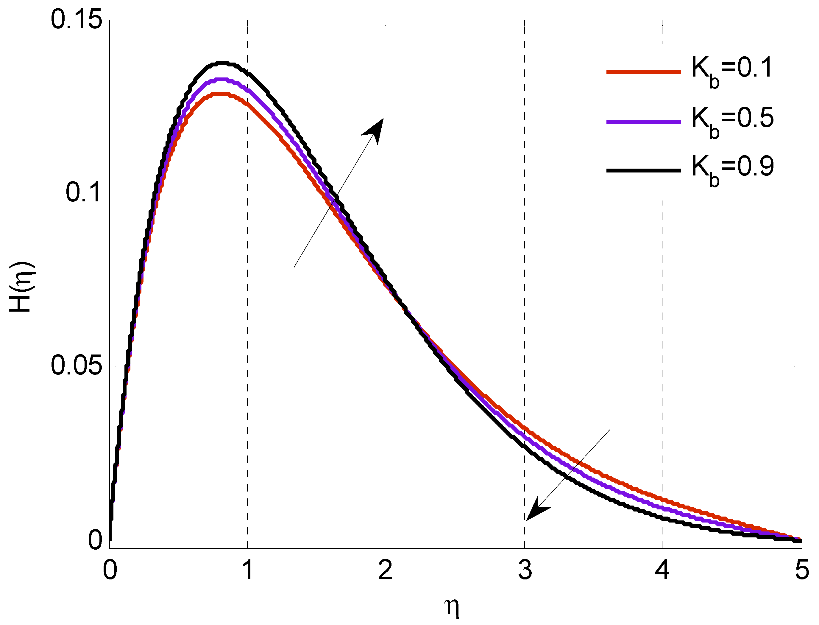
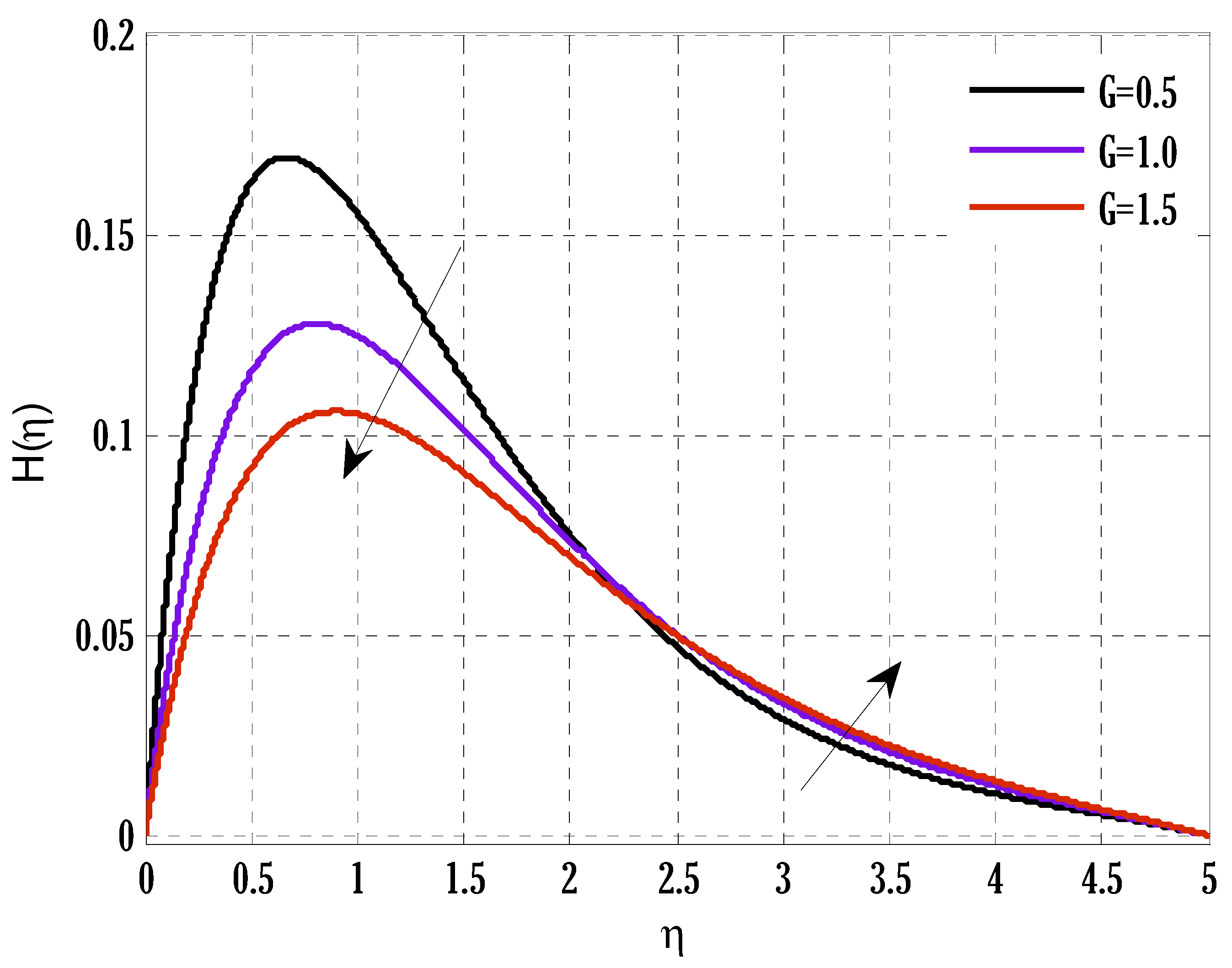
• The angular velocity displayed dual behavior as the coupling and microrotation parameters increased.
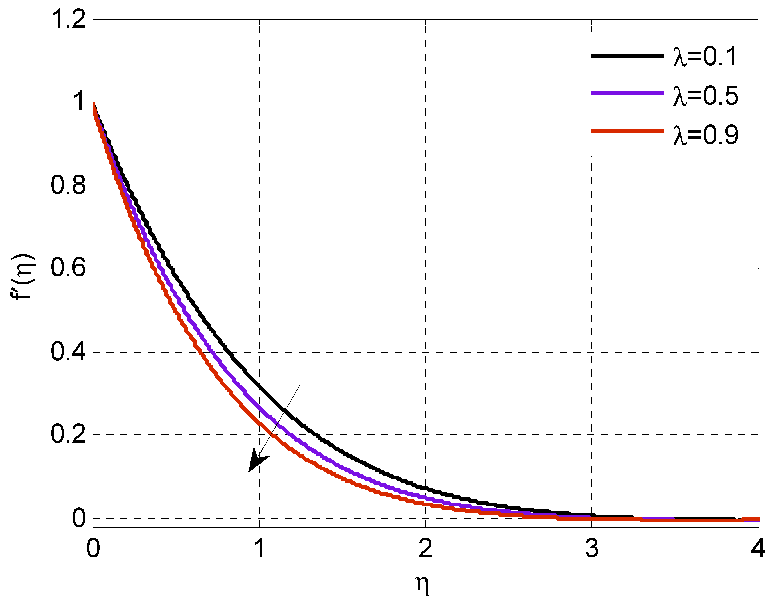
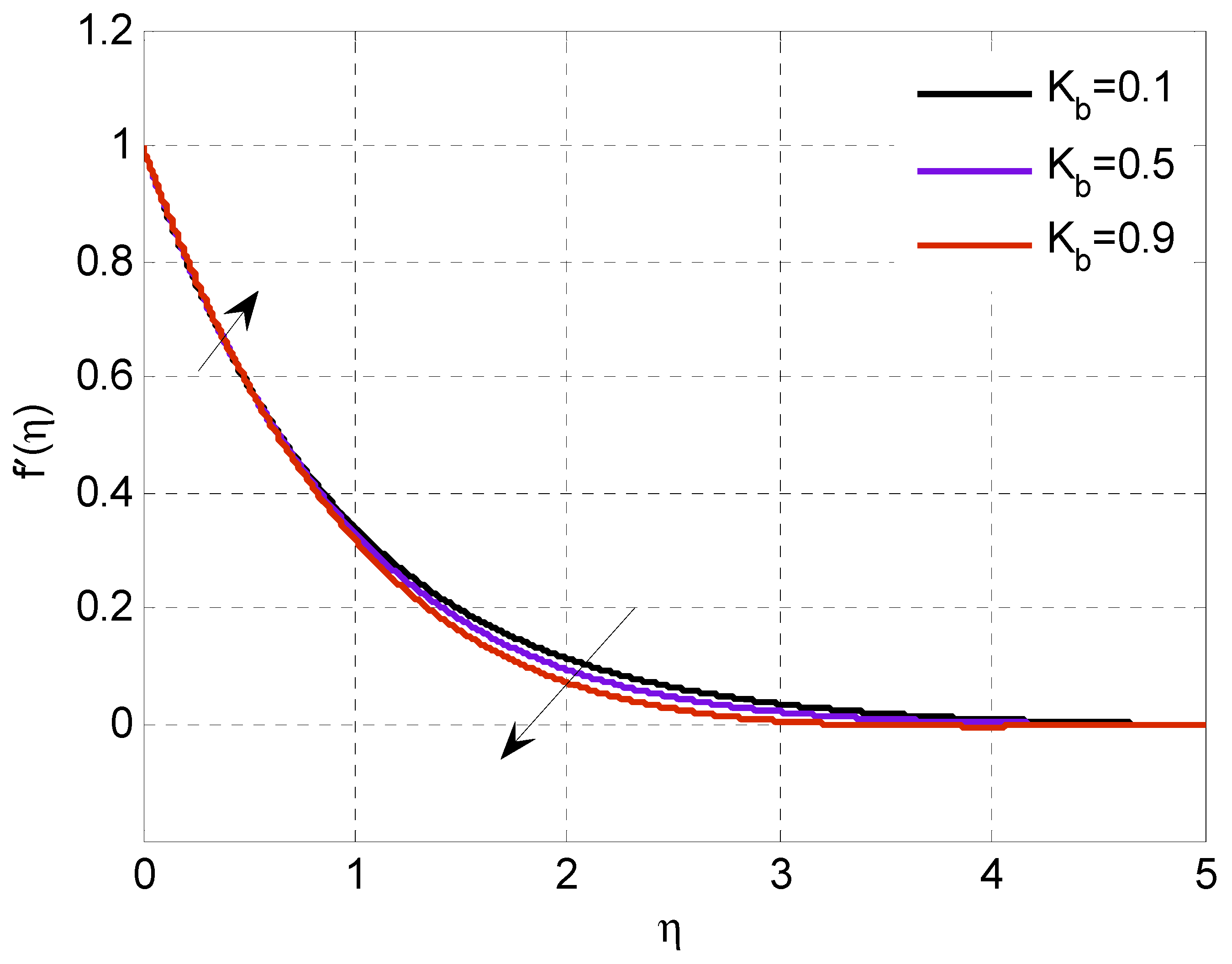
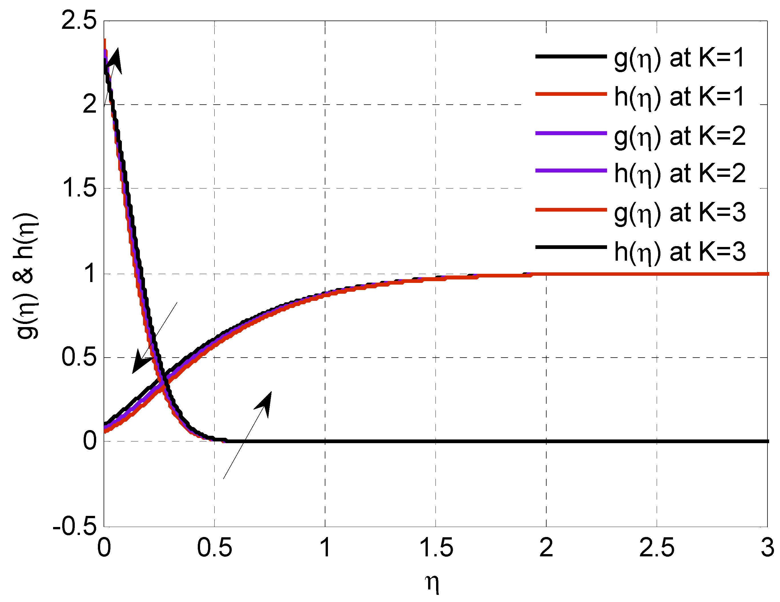
• The velocity profile also showed dual behavior as the coupling constant parameter increased.
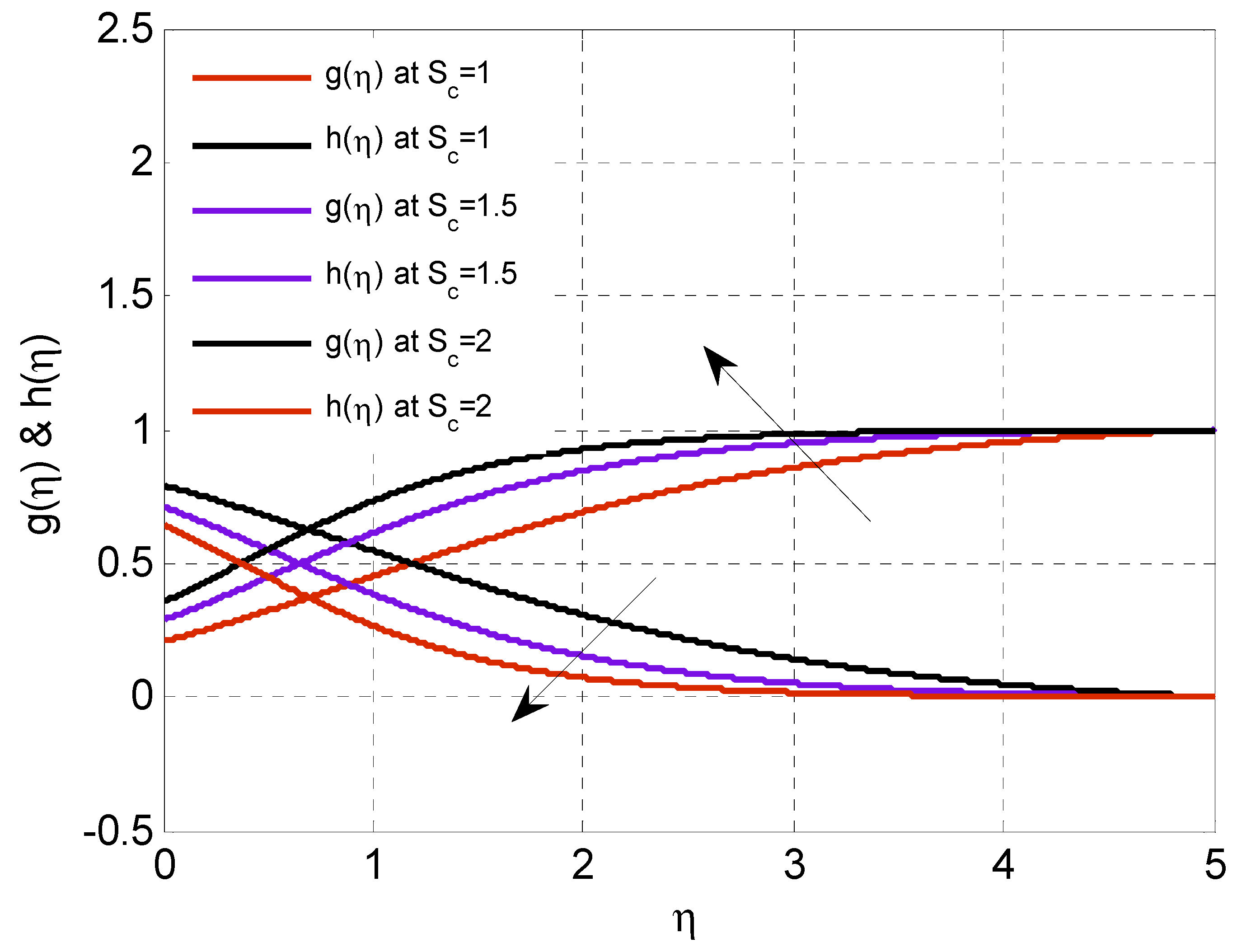
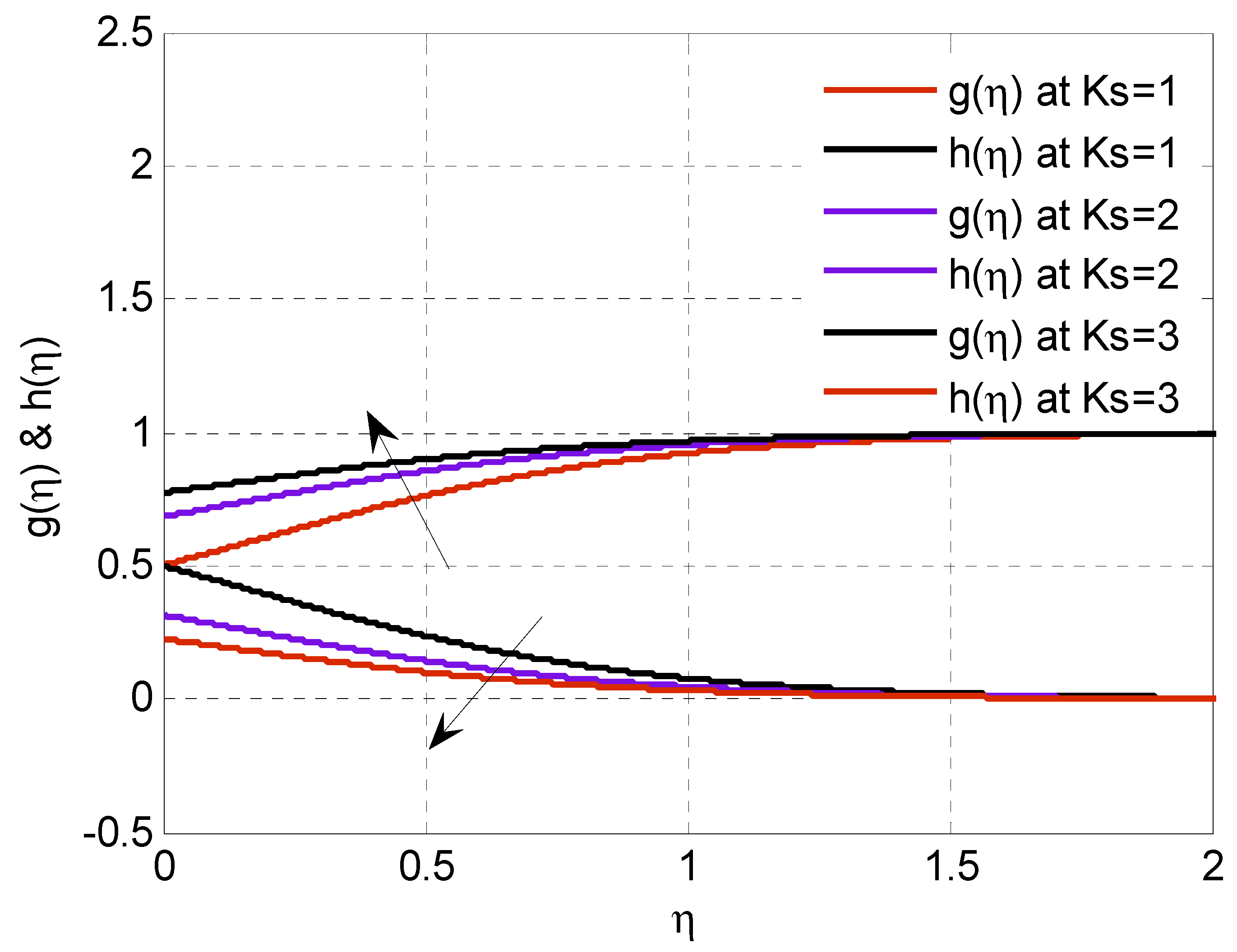
• The concentration profiles of species $A$ and $B$ displayed dual behavior as the values of the Schmidt number and the homogeneous and heterogeneous reaction parameters increased.

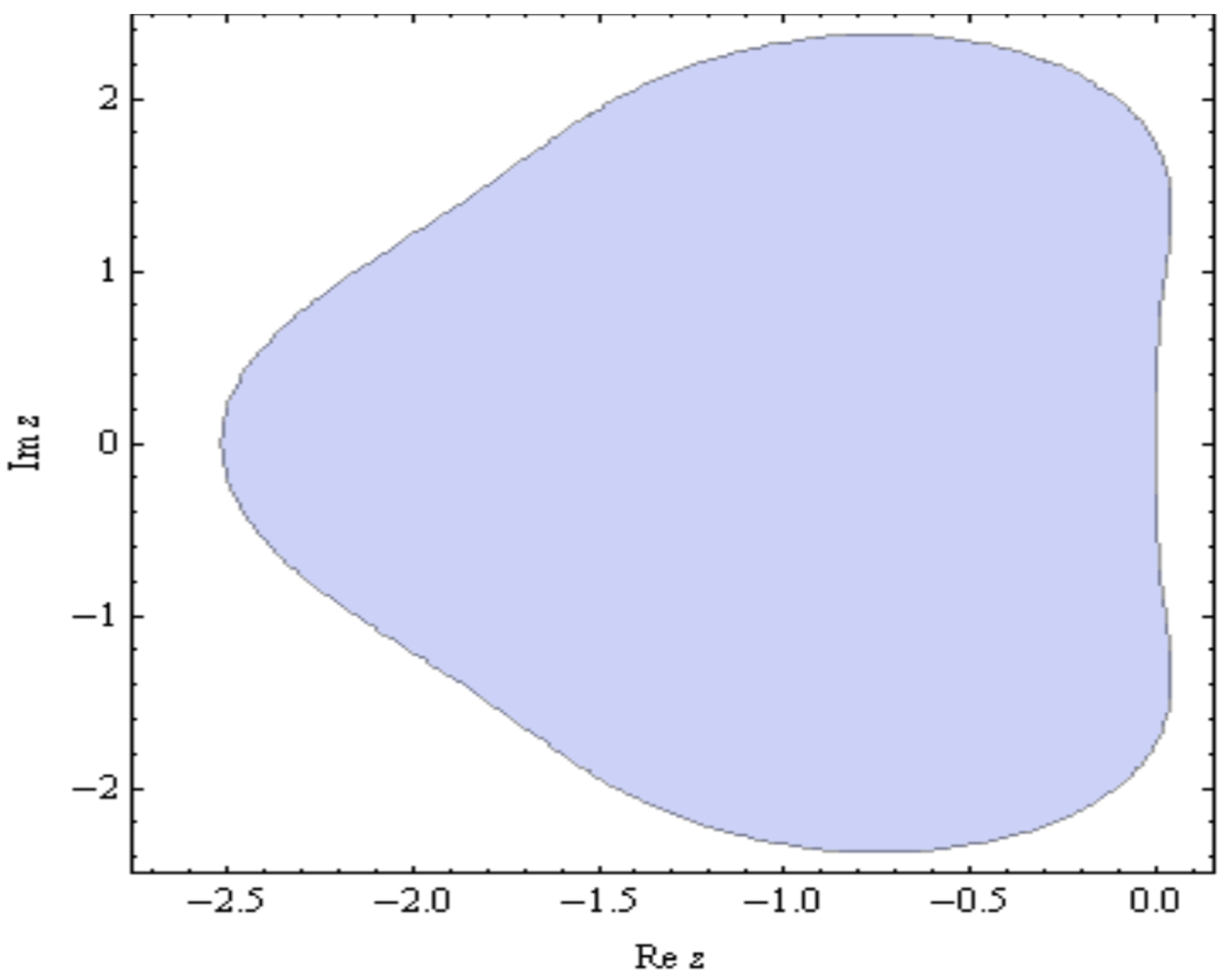
• The proposed scheme achieved a larger stability region than the existing Euler scheme.
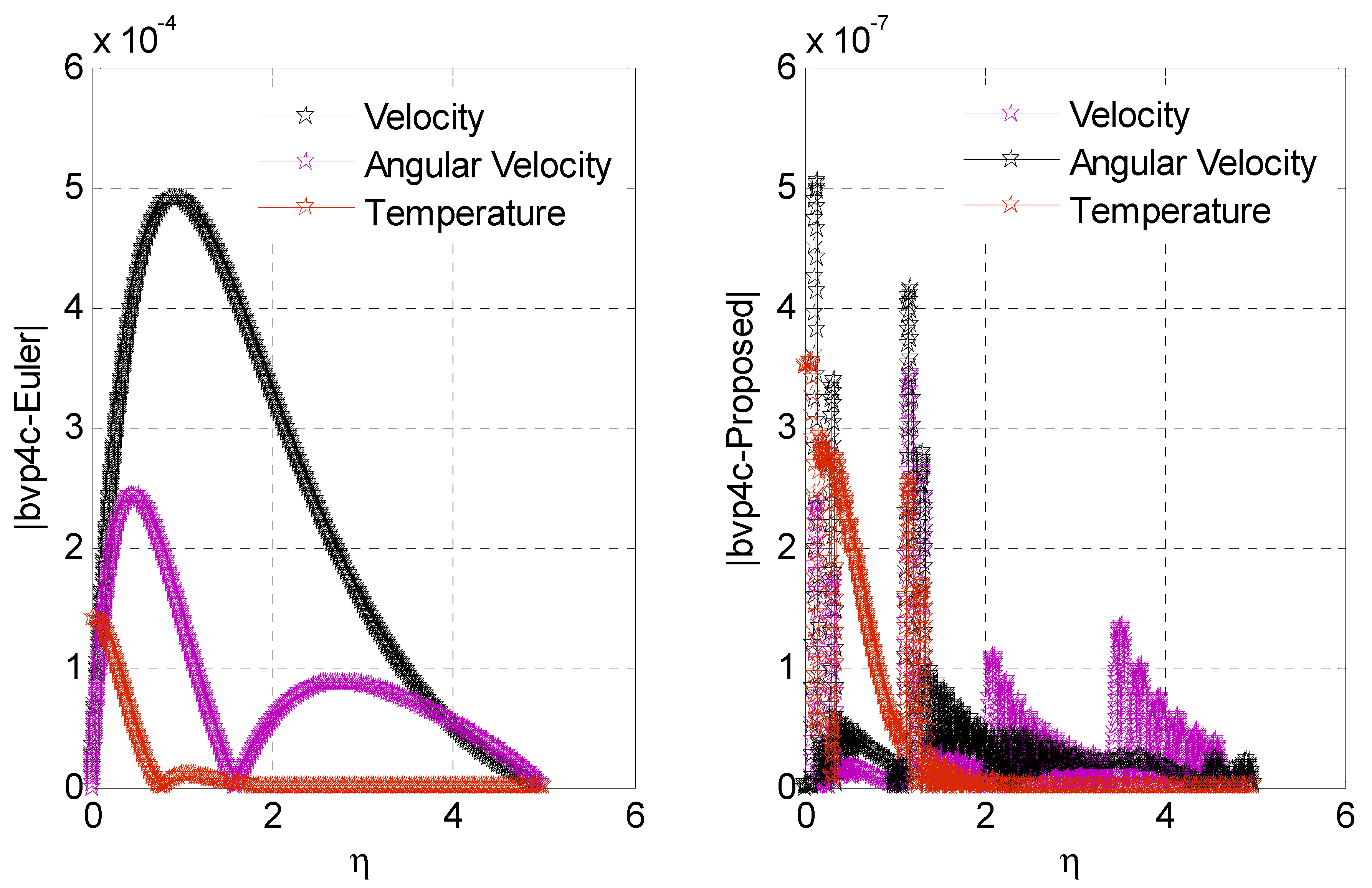
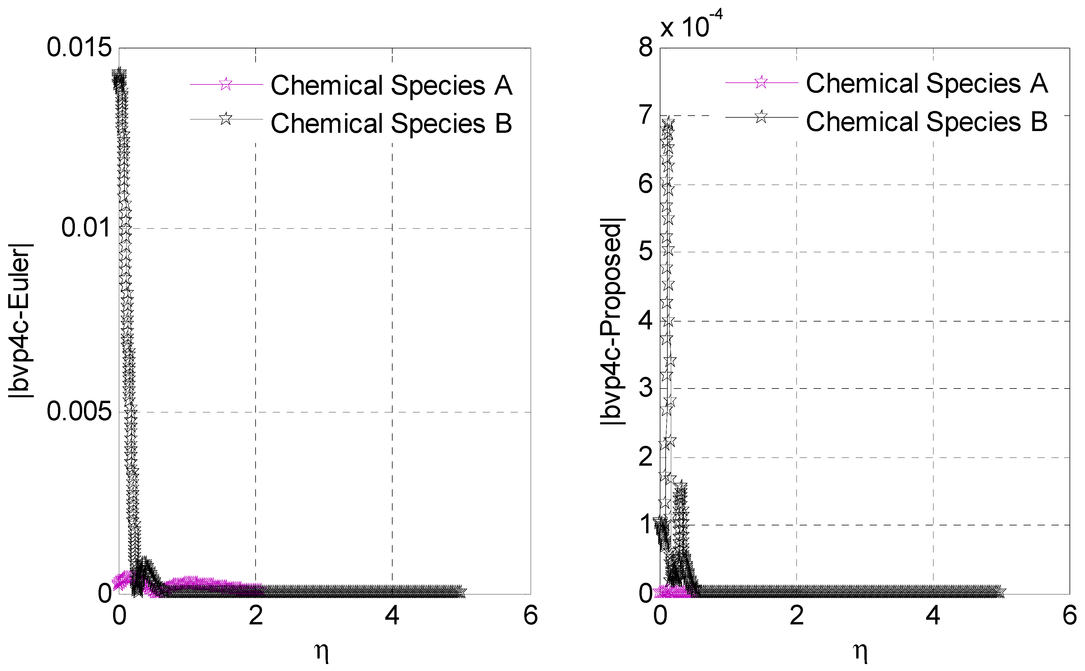
• The proposed scheme provided higher accuracy and a lower absolute error compared with the existing numerical scheme.

Following the completion of this investigation, it will be possible to recommend further applications for the current methods in addition to those already mentioned [44,45]. The proposed numerical scheme can be further applied to solve problems that arise in various science and engineering fields.

References

1. Eringen, A.C. Theory of micro polar fluids. J. Math. Mech. 1966, 16, 1–18. [Google Scholar]
2. Rees, D.A.S.; Pop, I. Free convection boundary layer flow of a micro polar fluid from a vertical flat plate. IMA J. Appl. Math. 1998, 16, 179–197. [Google Scholar] [CrossRef]
3. Lukaszewicz, G. Micropolar Fluids, Theory and Applications; Birkhauser: Boston, MA, USA, 1999. [Google Scholar]
4. Eremeyev, V.A.; Lebedev, L.P.; Altenbach, H. Foundations of Micropolar Mechanics; Springer: New York, NY, USA, 2013. [Google Scholar]
5. Beg, O.A.; Bhargava, R.; Rawat, S.; Kahya, E. Numerical study of micro polar convective heat and mass transfer in a non-Darcy porous regime with Soret and Dufour diffusion effects. Emir. J. Eng. Res. 2008, 13, 51–66. [Google Scholar]
6. Shafie, S.; Aurangzaib. Heat and mass transfer in a MHD non-Darcian micro polar fluid over an unsteady stretching sheet with non-uniform heat source/sink and thermophoresis. Heat Transf. Asian Res. 2012, 41, 601–612. [Google Scholar]
7. Srinivasacharya, D.; RamReddy, C. Mixed convection heat and mass transfer in a doubly stratified micro polar fluid. Comp. Ther. Sci. 2013, 5, 273–287. [Google Scholar] [CrossRef]
8. Noor, N.F.M.; Haq, R.U.; Nadeem, S.; Hashim, I. Mixed convection stagnation flow of a micro polar nanofluid along a vertically stretching surface with slip effect. Meccanica 2015, 50, 2007–2022. [Google Scholar] [CrossRef]
9. Tripathy, R.S.; Dash, G.C.; Mishra, S.R.; Hoque, M.M. Numerical analysis of hydromagnetic micro polar fluid along a stretching sheet embedded in porous medium with non-uniform heat source and chemical reaction. Eng. Sci. Technol. Int. J. 2016, 19, 1573–1581. [Google Scholar]
10. Mishra, S.R.; Baag, S.; Mohapatra, D.K. Chemical reaction and Soret effects on hydromagnetic micro polar fluid along a stretching sheet. Int. J. 2016, 19, 1919–1928. [Google Scholar]
11. Gibanov, N.S.; Sheremet, M.A.; Pop, I. Natural convection of micro polar fluid in a wavy differentially heated cavity. J. Mol. Liq. 2016, 221, 518–525. [Google Scholar] [CrossRef]
12. Nield, D.A.; Bejan, A. Convection in Porous Media, 4th ed.; Springer: New York, NY, USA, 2013. [Google Scholar]
13. Raptis, A. Flow of a micro polar fluid past a continuously moving plate by the presence of radiation: Technical note. Int. J. Heat Mass Transf. 1998, 41, 286–2866. [Google Scholar] [CrossRef]
14. Rahman, M.M.; Sattar, M.A. Magnetohydrodynamic convective flow of a micro polar fluid past a continuously moving vertical porous plate in the presence of heat generation/absorption. ASME J. Heat Transf. 2006, 128, 142–1552. [Google Scholar] [CrossRef]
15. Bhargava, R.; Sharma, S.; Takhar, H.S.; Beg, O.A.; Bhargava, P. Numerical solutions for micro polar transport phenomena over a nonlinear stretching sheet, Nonlinear Anal. Model. Control 2007, 12, 45–63. [Google Scholar]
16. Rashidi, M.M.; Erfani, E. A novel analytical method to investigate effect of radiation on flow of a magneto-micro polar fluid past a continuously moving plate with suction and blowing. Int. J. Model. Simul. Sci. Comput. 2010, 1, 219–238. [Google Scholar] [CrossRef]
17. Ramreddy, C.H.; Pradeepa, T. Spectral Quasi-linearization method for nonlinear thermal convection flow of a micro polar fluid under convective boundary condition. Nonlinear Eng. 2016, 5, 193–204. [Google Scholar] [CrossRef]
18. Shamshuddin, M.D.; Beg, O.A.; Ram, M.S.; Kadir, A. Finite element computation of multi-physical micro polar transport phenomena from an inclined moving plate in porous media. Ind. J. Phys. 2017, 92, 215–230. [Google Scholar] [CrossRef]
19. Hayat, T.; Khan, M.I.; Farooq, M.; Alsaedi, A.; Yasmeen, T. Impact of Marangoni convection in the flow of carbon-water nanofluid with thermal radiation. Int. J. Heat Mass Transf. 2017, 106, 810–815. [Google Scholar] [CrossRef]
20. Ferdows, M.; Shamshuddin, M.D.; Zaimi, K. Dissipative-radiative micro polar fluid transport in a non-Darcy porous medium with cross-diffusion effects. CFD Lett. 2020, 12, 70–89. [Google Scholar] [CrossRef]
21. Beg, O.A.; Ferdows, M.; Karim, M.E.; Hasan, M.M.; Beg, T.A.; Shamshuddin, M.D.; Kadir, A. Computation of nonisothermal thermo convective micro polar fluid dynamics in a Hall MHD generator system with nonlinear distending wall. Int. J. Appl. Comput. Math. 2020, 6, 42. [Google Scholar] [CrossRef]
22. Anathaswamy, V.; Sumathi, C.; Santhi, V.K. Analytical study on steady free convection and mass transfer flow of a conducting micro polar fluid. AIP Adv. 2021, 2378, 020017. [Google Scholar] [CrossRef]
23. Buongiorno, J. Convective transport in nanofluids. J. Heat Transf. 2006, 128, 240–250. [Google Scholar] [CrossRef]
24. Hayat, T.; Khan, M.I.; Waqas, M.; Alsaedi, A.; Khan, M.I. Radiative flow of micro polar nanofluid accounting thermophoresis and Brownian moment. Int. J. Hydrog. Energy 2017, 42, 16821–16833. [Google Scholar] [CrossRef]
25. Patel, H.R.; Singh, R. Thermophoresis, Brownian motion and nonlinear thermal radiation effects on mixed convection MHD micro polar fluid due to nonlinear stretched sheet in porous medium with viscous dissipation, Joule heating and convective boundary condition. Int. Commun. Heat Mass Transf. 2019, 107, 68–92. [Google Scholar] [CrossRef]
26. Sabir, Z.; Ayub, A.; Guirao, J.L.G.; Bhatti, S.; Shah, S.Z.H. The effect of activation energy and thermophoretic diffusion of nanoparticles on steady micro polar fluid along with Brownian motion. Adv. Mat. Sci. Eng. 2020, 2020, 2010568. [Google Scholar] [CrossRef]
27. Chamber, P.L.; Young, J.D. The effects of homogeneous 1st order chemical reactions in the neighborhood of a flat plate for destructive and generative reactions. Phys. Fluids 1958, 1, 48–54. [Google Scholar]
28. Khan, M.I.; Waqas, M.; Hayat, T.; Alsaedi, A. A comparative study of Casson fluid with homogeneous-heterogenous reactions. J. Colloid Interface Sci. 2017, 498, 85–90. [Google Scholar] [CrossRef]
29. Khan, M.I.; Alzahrani, F. Activation energy and binary chemical reaction effect in nonlinear thermal radiative stagnation point flow of Walter-B nanofluid: Numerical computations. Int. J. Mod. Phys. B 2020, 34, 2050132. [Google Scholar] [CrossRef]
30. Abbas, S.Z.; Khan, M.I.; Kadry, S.; Khan, W.A.; Israr-Ur-Rehman, M.; Waqas, M. Fully developed entropy optimized second order velocity slip MHD nanofluid flow with activation energy. Comput. Methods Programs Biomed. 2020, 190, 105362. [Google Scholar] [CrossRef]
31. Chaudhary, R.C.; Jha, A.K. Effects of chemical reactions on MHD micro polar fluid flow past a vertical plate in slip-flow regime. Appl. Math. Mech. 2008, 29, 1179–1194. [Google Scholar] [CrossRef]
32. Mahdy, A. Aspects of homogeneous-heterogeneous reactions on natural convection flow of micropolar fluid past a permeable cone. Appl. Math. Comput. 2019, 352, 59–67. [Google Scholar] [CrossRef]
33. Abouelregal, A.E.; Marin, M.; Alsharari, F. Thermoelastic Plane Waves in Materials with a Microstructure Based on Micropolar Thermoelasticity with Two Temperature and Higher Order Time Derivatives. Mathematics 2022, 10, 1552. [Google Scholar] [CrossRef]
34. Waqas, H.; Farooq, U.; Alshehri, H.M.; Goodarzi, M. Marangoni-bioconvectional flow of Reiner–Philippoff nanofluid with melting phenomenon and nonuniform heat source/sink in the presence of a swimming microorganisms. Math. Methods Appl. Sci. 2021, 1–19. [Google Scholar] [CrossRef]
35. Imran, M.; Farooq, U.; Waqas, H.; Anqi, A.E.; Safaei, M.R. Numerical performance of thermal conductivity in Bioconvection flow of cross nanofluid containing swimming microorganisms over a cylinder with melting phenomenon. Case Stud. Therm. Eng. 2021, 26, 101181. [Google Scholar] [CrossRef]
36. Alazwari, M.A.; Abu-Hamdeh, N.H.; Goodarzi, M. Entropy Optimization of First-Grade Viscoelastic Nanofluid Flow over a Stretching Sheet by Using Classical Keller-Box Scheme. Mathematics 2021, 9, 2563. [Google Scholar] [CrossRef]
37. Abdal, S.; Alhumade, H.; Siddique, I.; Alam, M.; Ahmad, I.; Hussain, S. Radiation and Multiple Slip Effects on Magnetohydrodynamic Bioconvection Flow of Micropolar Based Nanofluid over a Stretching Surface. Appl. Sci. 2021, 11, 5136. [Google Scholar] [CrossRef]
38. Rafique, K.; Alotaibi, H. Numerical Simulation of Williamson Nanofluid Flow over an Inclined Surface: Keller Box Analysis. Appl. Sci. 2021, 11, 11523. [Google Scholar] [CrossRef]
39. Khan, N.S.; Gul, T.; Islam, S.; Khan, I.; Alqahtani, A.M.; Alshomrani, A.S. Magnetohydrodynamic Nanoliquid Thin Film Sprayed on a Stretching Cylinder with Heat Transfer. Appl. Sci. 2017, 7, 271. [Google Scholar] [CrossRef]
40. Khan, N.S.; Kumam, P.; Thounthong, P. Computational Approach to Dynamic Systems through Similarity Measure and Homotopy Analysis Method for Renewable Energy. Crystals 2020, 10, 1086. [Google Scholar] [CrossRef]
41. Wang, C.Y. Free convection on a vertical stretching surface. J. Appl. Math. Mech. 1989, 69, 418–420. [Google Scholar] [CrossRef]
42. Khan, W.A.; Pop, I. Boundary-layer flow of a nanofluid past a stretching sheet. Int. J. Heat Mass Transfer 2010, 53, 2477–2483. [Google Scholar] [CrossRef]
43. Mabood, F.; Shamshuddin, M.D.; Mishra, S.R. Characteristics of thermophoresis and Brownian motion on radiative reactive micropolar fluid flow towards continuously moving flat plate: HAM solution. Math. Comput. Simul. 2022, 191, 187–202. [Google Scholar] [CrossRef]
44. Nawaz, Y.; Arif, M.S.; Abodayeh, K. A Compact Numerical Scheme for the Heat Transfer of Mixed Convection Flow in Quantum Calculus. Appl. Sci. 2022, 12, 4959. [Google Scholar] [CrossRef]
45. Nawaz, Y.; Arif, M.S.; Abodayeh, K. An explicit-implicit numerical scheme for time fractional boundary layer flows. Int. J. Numer. Methods Fluids 2022, 94, 920–940. [Google Scholar] [CrossRef]
Figure 1. Stability region of the proposed scheme.
Applsci 12 06072 g001
Figure 2. Geometry of the problem.
Applsci 12 06072 g002
Figure 3. Comparison of the proposed scheme with the forward Euler method for velocity, angular velocity, and temperature profiles using G = 1 ,   K b = 0.1 ,   λ = 0.1 ,   F r = 0.1 ,   P r = 7 ,   R d = 0.1 ,   Q = 0.1 ,   B i = 0.1 ,   and   N = 2040 .
Applsci 12 06072 g003
Figure 4. Comparison of the proposed scheme with the forward Euler method for species A and B using   G = 1 ,   K b = 0.1 ,   λ = 0.1 ,   F r = 0.1 ,   P r = 7 ,   R d = 0.1 ,   Q = 0.1 ,   B i = 0.1 ,   and   N = 2040 .
Applsci 12 06072 g004
Figure 5. Effect of porosity parameter on velocity profile using G = 1 ,   K b = 0.9 ,   F r = 0.1 , and N = 3040 .
Applsci 12 06072 g005
Figure 6. Effect of inertia coefficient on velocity profile using G = 1 ,   K b = 0.9 ,   F r = 0.1 ,   and   N = 3040 .
Applsci 12 06072 g006
Figure 7. Effect of coupling parameter on velocity profile using G = 1 ,   λ = 0.1 ,   and   F r = 0.1 .
Applsci 12 06072 g007
Figure 8. Effect of coupling parameter on angular velocity using G = 1 ,   λ = 0.1 ,   F r = 0.1 ,   and   N = 3040 .
Applsci 12 06072 g008
Figure 9. Effect of microrotation parameter on angular velocity using K b = 0.01 ,   λ = 0.1 ,   F r = 0.1 ,   and   N = 3040 .
Applsci 12 06072 g009
Figure 10. Effect of Biot number on temperature profile using G = 1 ,   K b = 1 ,   λ = 0.5 ,   F r = 0.1 ,   P r = 4 ,   R d = 0.1 ,   Q = 0.3 ,   and   N = 3040 .
Applsci 12 06072 g010
Figure 11. Effect of heat source parameter on temperature profile using G = 1 ,   K b = 1 ,   λ = 0.5 ,   F r = 0.1 ,   P r = 4 ,   R d = 0.1 ,   B i = 0.5 ,   and   N = 3040 .
Applsci 12 06072 g011
Figure 12. Effect of Schmidt number on concentration profiles of species A and B using G = 1 ,   K b = 1 ,   λ = 0.5 ,   F r = 0.1 ,   K = 1 ,   δ = 1 ,   K 2 = 1 ,   and   N = 3040 .
Applsci 12 06072 g012
Figure 13. Effect of homogeneous reaction parameter on concentration profiles of species A and B using G = 1 ,   K b = 1 ,   λ = 0.5 ,   F r = 0.1 ,   K 2 = 0.1 ,   δ = 0.1 ,   S c = 4 ,   and   N = 3040 .
Applsci 12 06072 g013
Figure 14. Effect of heterogeneous reaction parameter on concentration profiles of species A and B using G = 1 ,   K b = 1 ,   λ = 0.5 ,   F r = 0.1 ,   K = 1 ,   δ = 1 ,   S c = 4 ,   and   N = 3040 .
Applsci 12 06072 g014