
IMNets: Deep Learning Using an Incremental Modular Network Synthesis Approach for Medical Imaging Applications


1
Department of Electrical and Computer Engineering, University of Dayton, 300 College Park, Dayton, OH 45469, USA
2
Sensors and Software Systems Division, University of Dayton Research Institute, 1700 South Patterson Blvd., Dayton, OH 45409, USA
*
Author to whom correspondence should be addressed.
Appl. Sci. 2022, 12(11), 5500; https://doi.org/10.3390/app12115500
Submission received: 23 April 2022
/
Revised: 22 May 2022
/
Accepted: 27 May 2022
/
Published: 29 May 2022
(This article belongs to the Special Issue Artificial Intelligence in Medical Imaging: The Beginning of a New Era)
Abstract
:Deep learning approaches play a crucial role in computer-aided diagnosis systems to support clinical decision-making. However, developing such automated solutions is challenging due to the limited availability of annotated medical data. In this study, we proposed a novel and computationally efficient deep learning approach to leverage small data for learning generalizable and domain invariant representations in different medical imaging applications such as malaria, diabetic retinopathy, and tuberculosis. We refer to our approach as Incremental Modular Network Synthesis (IMNS), and the resulting CNNs as Incremental Modular Networks (IMNets). Our IMNS approach is to use small network modules that we call SubNets which are capable of generating salient features for a particular problem. Then, we build up ever larger and more powerful networks by combining these SubNets in different configurations. At each stage, only one new SubNet module undergoes learning updates. This reduces the computational resource requirements for training and aids in network optimization. We compare IMNets against classic and state-of-the-art deep learning architectures such as AlexNet, ResNet-50, Inception v3, DenseNet-201, and NasNet for the various experiments conducted in this study. Our proposed IMNS design leads to high average classification accuracies of 97.0%, 97.9%, and 88.6% for malaria, diabetic retinopathy, and tuberculosis, respectively. Our modular design for deep learning achieves the state-of-the-art performance in the scenarios tested. The IMNets produced here have a relatively low computational complexity compared to traditional deep learning architectures. The largest IMNet tested here has 0.95 M of the learnable parameters and 0.08 G of the floating-point multiply–add (MAdd) operations. The simpler IMNets train faster, have lower memory requirements, and process images faster than the benchmark methods tested.
1. Introduction
1.1. Background
Recently, deep learning with convolutional neural networks (CNNs) has proven to be highly effective for computer-aided detection (CAD) in medical image analysis. The trend in CNN architectures recently has been towards ever deeper and wider networks with dense connectivity. For example, ViT-G/14 [1] and ViT-MoE-15B [2] were the top two CNN architectures in the ImageNet Large-Scale Visual Recognition Challenge (ILSVRC) competition in 2021 [3]. The ViT-G/14 and ViT-MoE-15B architectures contain 1.843 G and 14.70 G parameters, respectively. Furthermore, ViT-G/14 requires 965.3 G floating point operations (FLOPs) per single image, which is a very computationally costly and power-hungry solution. Perhaps even more significantly, larger networks require more training data to be able to generalize to new data [4]. In many medical image analysis applications, access to properly-labeled truth imagery is limited, especially for rare diseases [4]. Data collection and truthing in medical imaging can be cost-intensive, time-consuming, and requires expert analysis. Transfer learning can help to reduce the amount of application-specific data required for training. However, large amounts of data may still be needed to obtain the desired reproducibility and generalizability, even with transfer learning [5,6]. Data augmentation is another approach to dealing with limited training data. However, data augmentation can be very challenging in some medical imaging modalities such as chest radiographs [7].
Modular CNN architectures are a promising approach for complex problem-solving that may be able to help address the challenges described above. Some modular methods are inspired by the structure and function of the human brain. Recent findings in neuroscience reveal a high level of modularity and hierarchy of neural structure in the human brain [8]. In the early 1980s, neuroscientific research categorized the central nervous system (CNS) in the human brain as a massively parallel and self-organizing modular system [9,10,11]. The CNS consists of distinctive regions. Each region develops as a functional module. The modules are densely connected and interact with one another to accomplish complex perception and cognitive tasks in an efficient manner [9]. Traditional CNN architectures often use repeating structures such as layers or groups of layers. However, the networks are generally trained as one monolithic entity with all learnable parameters being updated simultaneously.
1.2. Applications
Malaria is a deadly disease that is considered endemic in many countries around the world [12]. In the year 2020, the World Health Organization (WHO) reported an estimated 229 million cases of malaria worldwide, which caused an estimated 409,000 deaths [13]. Malaria occurs in humans via protozoa within the blood cells of the genus Plasmodium. These parasites are transmitted by the bite of a female Anopheles mosquito [14]. The mosquito bite injects the Plasmodium into the affected person’s blood, and then the Plasmodium parasites pass quickly to the liver to mature and replicate [15]. The most common imaging modality for detecting parasites in a thin blood smear sample is microscopical imaging [16]. While microscopy is relatively low-cost and widely accessible, diagnosis efficiency depends on the experience of parasitologists [17]. False-positive or false-negative diagnoses can lead to inappropriate or unnecessary prescriptions that can cause side effects in patients. Due to the global shortage of parasitologists in impoverished urban areas accurately processing the large number of specimens encountered is not always possible [18,19]. Thus, CAD systems can be highly beneficial in this application.
Another disease for which CAD systems can help by providing accurate early detection is diabetic retinopathy (DR). This condition is a typical development of diabetes, affecting the retina’s small blood vessels, leading to vision deterioration [20]. The research described in [21] studies the offloading footwear to prevent and lower mortality rates in high-risk diabetic feet. A recent study has reported that DR affects the vision of 2.6 million people in the world [20,22]. Several retinal imaging systems can be utilized to detect the indication of diabetic retinopathy, including color fundus photography, fluorescein angiography, B-scan ultrasonography, and optical coherence tomography [23]. The retina images that we use in our study have been captured using fundus photography under a variety of imaging conditions. Early-stage diagnosis of DR grading is integral to prevent the occurrence of blindness. Hence, CAD systems could help save millions of people from potentially preventable vision loss and blindness by improving early detection.
The third and final application we consider here is pulmonary tuberculosis (TB). This disease is a significant public health issue causing more than 9 million expected new cases and roughly 1.4 million deaths every year [24]. The detection of TB on chest radiographs (CRs) is essential for diagnosing TB. Chest radiography imaging (e.g., X-ray or computed tomography (CT) imaging) is easy to perform with fast diagnosis and has a high sensitivity for diagnosing TB infection. However, CRs are the fastest and most affordable form of imaging and require significantly less radiation, data memory, and processing time than CT scans [25]. The WHO recommends using CRs to screen and triage people for TB [26]. Note that CRs are among the first procedures of examination related to suspects’ lung disease. They are low-cost and widely accessible for health care providers. The use of CAD systems for TB detection can help radiologist workflow so they may be able to process more cases with greater accuracy.
1.3. Related Works
Various approaches have been proposed in the literature for medical imaging CAD systems, including those for malaria, DR and TB [27,28,29,30,31,32,33,34,35,36,37,38,39,40,41,42,43]. The work described in [28] aims to improve malaria parasite detection using tiny red blood smear patches; they utilize several existing deep convolutional neural networks in place of handcrafted feature extraction. The study claims that using preprocessing techniques such as standardization, normalization, and stain normalization does not improve the overall performance model. An effective multi-magnification deep residual neural network (MM-ResNet) has been trained on microscopic phone image datasets of malaria blood smears obtained from the AI research group at Makerere University. The MM-ResNet end-to-end framework takes three different images of size as inputs. It concatenates each ResNet at the second to the last layer, followed by a final fully connected layer [29]. VGG-16 and VGG-19 have been trained on the National Institutes of Health (NIH) malaria dataset using hyperparameter tuning techniques described in [30], the CNN used to automate the screening of malaria in low-resource countries achieves an accuracy of 0.9600. A survey article on image analysis of microscopic blood slides uses many machine learning techniques for malaria detection [31]. Patient information was considered, such as nationality, age, gender, body region, and symptomatology of a patient as a part of features engineering for malaria detection. Furthermore, they examined six machine learning algorithms, including support vector machine (SVM), random forest (RF), multilayer perceptron (MLP), AdaBoost, gradient boosting (GB), and CatBoost to classify infected and non-infected cells [32]. A fast CNN architecture present in [33] is used to classify thin blood smeary images. This paper studied the performance of transfer learning approaches for various pre-trained CNN architectures, including AlexNet, ResNet, VGG-16, and DenseNet. Furthermore, they studied the performance of a traditional machine learning algorithm using a bag-of-features model with SVM.
Many deep learning methods, originally proposed for the ILSVRC [44], have been adapted to the medical image application. Among these are meta-algorithms for DR detection, which combine five CNN architectures into one predictive model [34]. Zhang et al. [35] fine-tuned ResNet that pre-trained on the ImageNet dataset. The work described in [36] developed a real-time smartphone app to detect and classify DR by using a pre-trained Inception v3 model with a transfer learning technique. A hybrid machine learning technique is introduced in [37] to detect and grade DR severity level. The study compares simple transfer learning-based approaches using seven pre-trained networks. Another fine-tuned, pre-trained approach for DR detection is presented in [38] using a cosine annealing strategy to decay the learning rate. The transfer learning method for TB described in [39] was used to neutrophil cluster detection. An automatic TB screening system presented in [40] is based on transfer learning from lower convolutional layers of pre-trained networks. The method in [42] uses a simple segmentation approach to classify the images’ foreground and background. The segmented objects are then fed to a trained CNN to classify the objects into bacilli and non-bacilli. A total of four state-of-the-art 3D CNN models are used to detect the spatial location of lesions and classify the candidates into miliary, infiltrative, caseous, tuberculoma, and cavitary types in [43]. A multi-strategy fast non-dominated solution ranking algorithm with high robustness is described in [45].
Of particular relevance to our work is the Net2Net method introduced by Chen et al. [46]. The method is modular in that it allows two neural networks to mimic the behavior of a more complex network. The Net2Net is an effective technique to transfer the prior knowledge from a trained neural network (teacher network) to a new deeper, or wider network (student network). The Net2Net approach implemented in [46] combines two neural networks to form a larger network. It does so by either increasing the width or the depth of the network. The method replicates the teacher network weights to expand the student network size either in width or depth. After replicating, the new addition is initialized to be an identity network. This method can guarantee that the student model can perform just as well as the teacher network at the start of training. The student model obtains good accuracy much faster than training the larger network from scratch. While Net2Net is a practical and innovative approach that works very well for knowledge transfer, the Net2Net method has a few limitations. For example, the current implementation of Net2Net in [46] uses only two networks. Furthermore, there are restrictions on the networks in terms of kernel sizes, activation functions, and initialization, so as to achieve the stated network properties.
Another related modular technique that is designed to work with small amounts of training data is presented in [47]. The module uses the entire CNN network as modules. It combines pre-trained modules with untrained modules, allowing the new network to learn discriminative features. The pre-trained models VGG-16 and ResNet were used. The module fine-tunes the VGG-16 model on the Stanford Cars dataset by replacing the last three layers with two consecutive fully connected layers, softmax, and loss function. Then, the module merges the fixed VGG16 features with a ResNet. The output of both models was then fed to two fully connected layers, softmax, and loss function.
1.4. Contributions
In this paper, we propose a novel and a computationally efficient deep learning approach for medical image analysis using CNNs. We refer to our approach as Incremental Modular Network Synthesis (IMNS), and the resulting CNNs as Incremental Modular Networks (IMNets). Our IMNS approach is to use small network modules that we call SubNets that are capable of generating salient features for a particular problem. Compared with other modular methods in the literature, our IMNS approach has some distinct features. First, we begin with small compact SubNet modules to keep the computational complexity low. Second, we build networks using both series and parallel arrangements in a sequential incremental manner. This provides freedom of building nearly any custom network without restriction. The essential feature of our approach is that we start by training one small SubNet and lock in those network parameters. We add depth or width to that initial network and train only the new SubNet at a time. We do this incrementally until we achieve the desired network performance. Our approach guarantees the freedom of choosing any configuration for the initial network, including the number of layers, the kernel size, series network incremental or parallel network incremental. To the best of our knowledge this kind of modular network synthesis approach has not been previously employed in medical image CAD applications.
1.5. Paper Organization
2. Materials
In this paper, we utilized three different datasets to study the performance of our method. First, we utilized a publicly available dataset provided by the NIH [48] for malaria detection. Second, we used the publicly available Asia Pacific Tele-Ophthalmology Society (APTOS) 2019 blindness detection challenge dataset [49] for DR detection. Lastly, for TB detection, we make use of a publicly available Shenzhen chest radiograph dataset [50].
2.1. Malaria Dataset
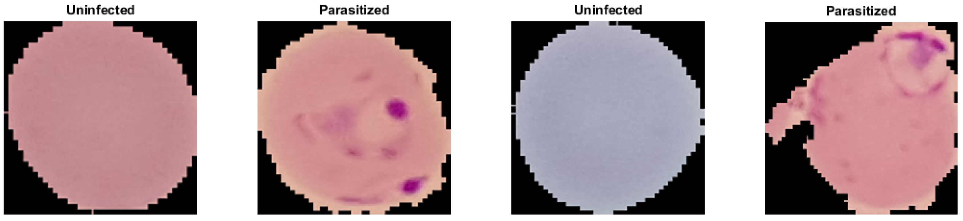
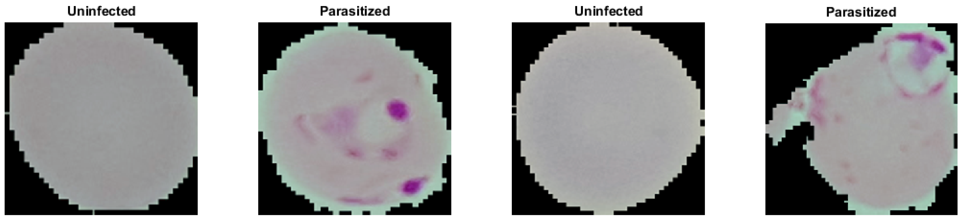
Malaria dataset provided segmented cell samples that have been obtained from the thin blood smear slide images from the Malaria Screener research activity [48]. According to the NIH, all images were manually labeled by a proficient slide reader at the Mahidol-Oxford Tropical Medicine Research Unit in Bangkok, Thailand [48]. The dataset comprises 27,558 cell images with equal representation of parasitized and uninfected cells. We randomly divided the dataset into 80% for training and 20% for testing representations regarding each class. Moreover, we split the training dataset into 90% and 10% for training and validation sets. Table 1 shows the hold-out validation distribution of the malaria dataset and the number of training, validation, and testing samples. Figure 1 shows the raw sample, which tends to have different illumination conditions. Therefore, we pre-processed all images by applying the color constancy technique [51] to ensure the perceived color of each image remained the same under different illumination conditions. Results of the color constancy outputs for the input images in Figure 1 are shown in Figure 2.
2.2. Diabetic Retinopathy Dataset
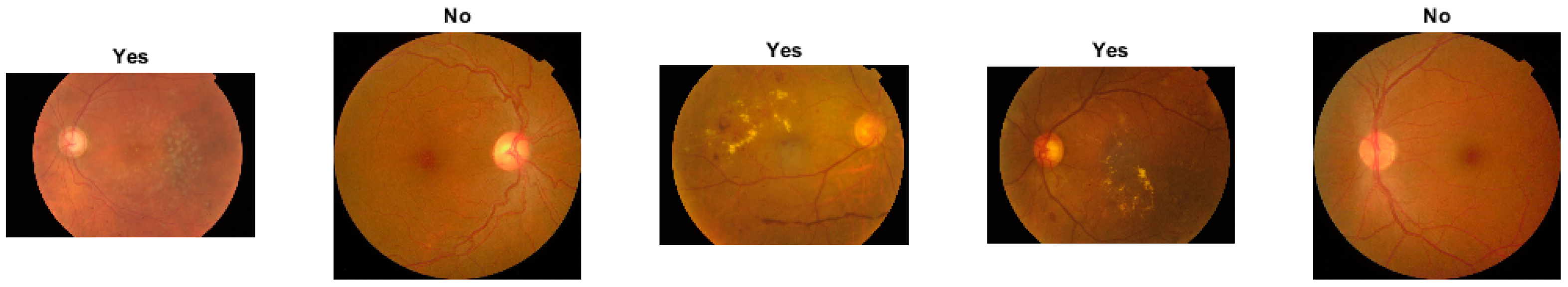
The technicians in the Aravind Eye Hospital in India have collected retinal images from patients who live in rural areas aiming to detect and prevent diabetic retinopathy [49]. Trained doctors then reviewed these images to provide the diagnosis. This APTOS 2019 dataset consists of 5590 retinal image samples. The dataset has been split up into training and testing cases by the challenge host organization. The training dataset is comprised of 3662 samples. The testing dataset contains 1928 samples, but the labels for the testing dataset are not publicly available yet. The dataset contains five classes, including No DR and the other four stages of DR (Mild DR, Moderate DR, Proliferative DR, and Severe DR). In this study, we grouped the dataset into two possible disease categories, normal and DR classes. The four types of DR diseases have been grouped together in the DR class. Moreover, since the testing dataset labels are not available, we solely used the training dataset provided as part of the APTOS 2019 challenge. The training dataset was randomly split into 80% for training and 20% for testing. Then, the training dataset is divided into 90% and 10% for training and validation sets. Table 1 shows the number of training, validation, and testing samples for DR dataset. Figure 3 shows random samples of labeled images from the APTOS 2019 DR dataset after we grouped them into two classes.
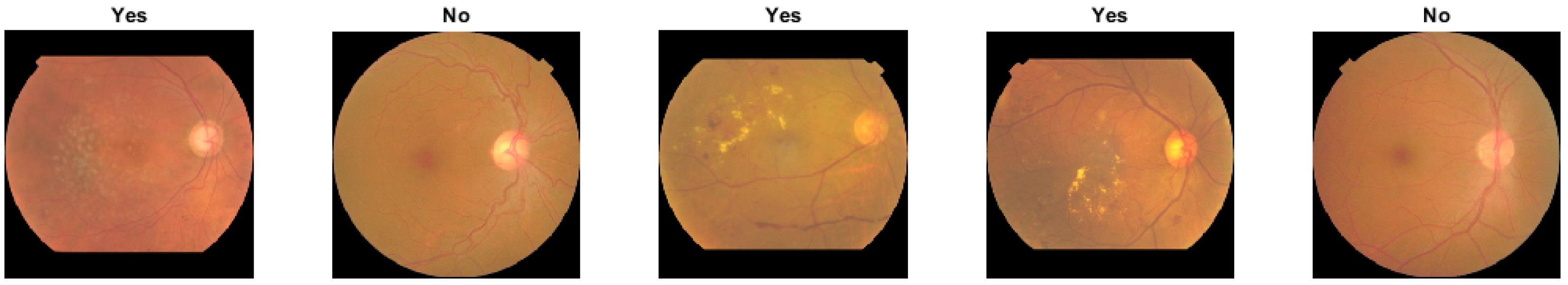
We have studied and visualized the dataset, and we found that the images contain artifacts, varying sizes, different optic nerve angles, and were captured under different lighting conditions so that some are underexposed or overexposed. To handle this variability, we propose applying pre-processing techniques to seek to normalize the data for these factors. The eye image pre-processing technique consists of four steps:
- We find the mask of the orange portion of the eye and separate it from the black background.
- We locate the optic nerve that appears as a bright disk in the images. This is achieved by applying a Gaussian low-pass filter with a spatial standard deviation approximately equal to the radius of the optic nerve disk. The brightest pixel after the blurring operation generally is located near the center of the optic nerve.
- We compare the location of the optic nerve center to the center of the eye mask to determine the orientation of the eye. We then rotate the image so that optic nerve is consistently on the right of center in the resulting image.
- Finally, we crop, zero pad, and interpolate to obtain the same size images. We do so in such a way as to not change the aspect ratio of image, as this would contaminate the geometric integrity of the data.
2.3. Tuberculosis Dataset
We utilized the Shenzhen dataset [50] for TB detection that holds 326 normal CR cases and 326 CR with active pulmonary tuberculosis. The chest radiograph images in the Shenzhen dataset have been collected by Shenzhen No. 3 Hospital in Shenzhen, Guangdong province, China. In our experimental study using these data, we perform a hold-out validation. We randomly divide the dataset into groups of 72% for training, 8% for validation, and 20% for testing. Table 1 shows the hold-out validation distribution of the TB dataset.
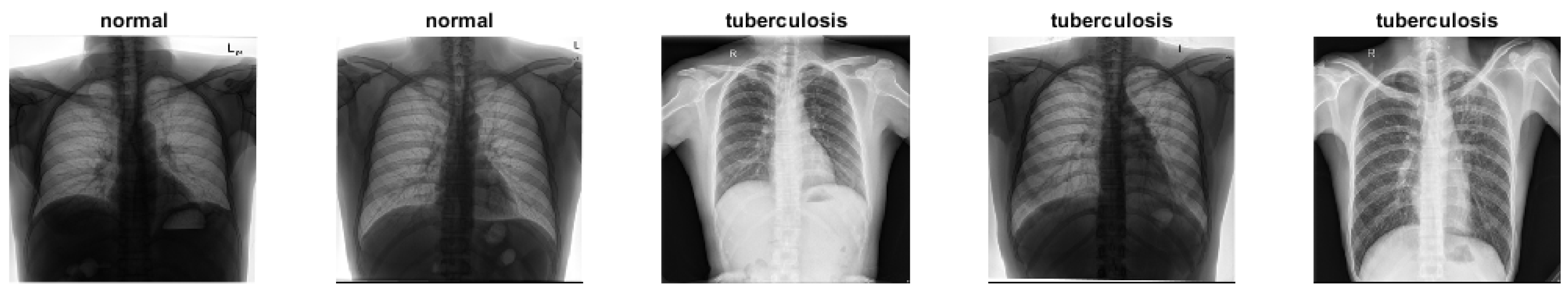
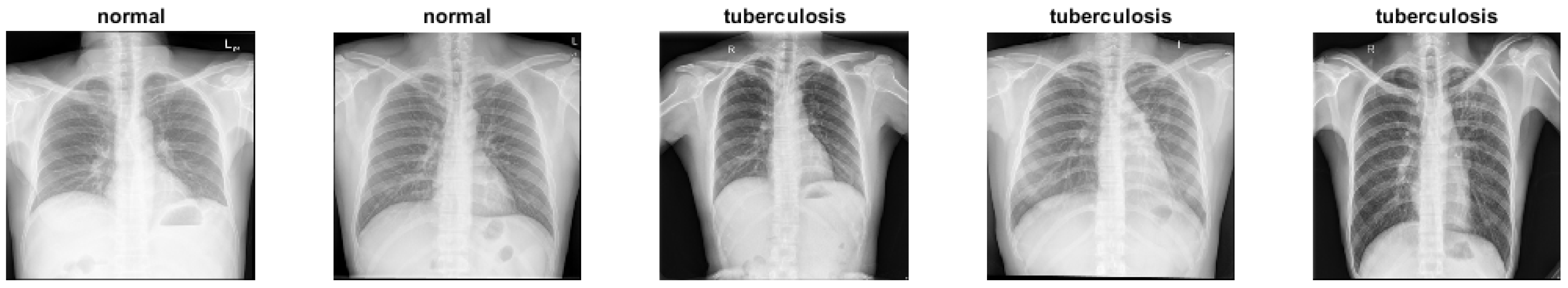
The CR images are in JPEG format with a resolution of pixels. Some example labeled CR images from the Shenzhen dataset are shown in Figure 5. Figure 5 shows that some CR samples in the dataset have an inverse intensity polarity. We find that it is critical to network performance to make all of the CR images have the same polarity. Therefore, all cases are reviewed manually and inverted as needed. For this research, we converted all the images to a size of . The example images Figure 5 after the corrective inversion processing are shown in Figure 6.
3. Methods
In this section, describe the details of the proposed IMNS method. We begin with an overview. Next, we explain the details of each SubNet and how they work together. Then, we present the specific IMNet architecture used in our experimental study. Finally, we end this section with a discussion of our network training process.
3.1. Overview
The inspiration for the IMNS approach comes from children’s building blocks. We propose that CNN architectures can be assembled using modular components in a manner that is akin to building a structure with a child’s building blocks. Each module requires only an incremental additional training process. This allows for a potentially massive network without the computational cost of training the final network at one time, which could be prohibitive. The proposed IMNS uses a unique hybrid learning strategy that successfully combines multiple SubNet to produce complementary information.
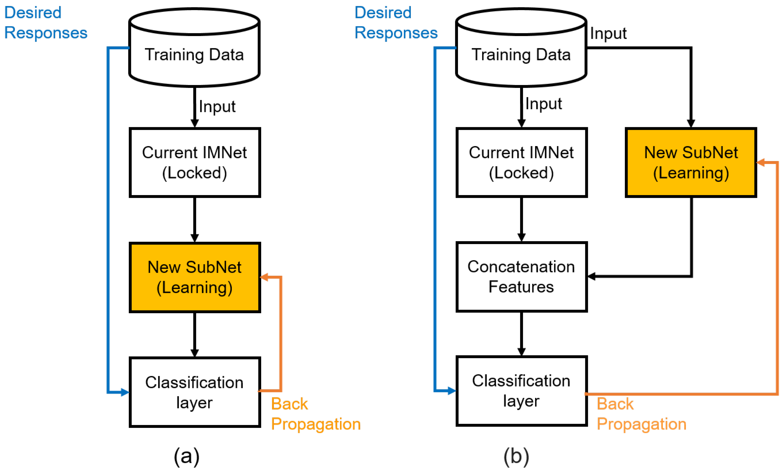
In our approach, each SubNets module is added incrementally onto existing architecture in either a series or parallel fashion. These two scenarios are illustrated in Figure 7. Note that in Figure 7a, a new SubNet is added in series to the feature computation layers of the current IMNet. The classification layers are moved to the end of the network as shown. Note also that the learnable parameters of the current IMNet are locked-in, and only the learnable parameters of the new SubNet are updated. For large networks, this dramatically reduces the computational demands of the back-propagation updates. At some stages of the IMNS process, the user may wish to expand the network in parallel. This is shown in Figure 7b. As before the classification layers are moved to the end, and only the new Subnet is updated in the back-propagation learning algorithm. One new operation that is needed here is the concatenation layer that takes the feature maps generated from the current IMNet and concatenates them with the feature maps generated by the new SubNet. We concatenate these feature maps in the channel dimension.
3.2. SubNet Architecture
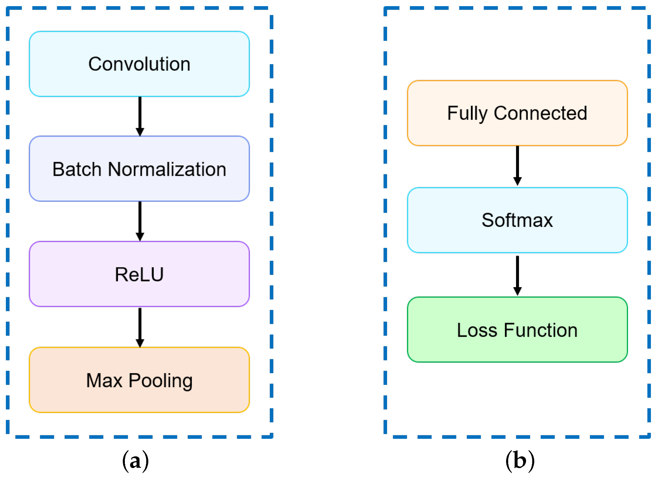
The individual SubNet architectures considered here are shown in Figure 8. The feature generating SubNets are comprised of a selected number of the layer groups shown in Figure 8a. The classification layers are shown in Figure 8b. Figure 8a shows the convolutional layer structure where each convolutional layer followed by a batch normalization layer, rectified linear units (ReLU), and max pooling of window size with a stride of 2 to downsample the feature maps. Note that the number and size of convolution filters present in each layer may differ. The classification block consists of one fully connected layer, softmax function, and cross-entropy loss function as shown in Figure 8b.
Let us formally define the output of a SubNet made up of layer groups such as those shown in Figure 8a followed by an L’th classification layer as shown in Figure 8b. To begin, let us define one minibatch of input data as
where is the n’th exemplar from the minibatch. These inputs represent potentially multi-channel images with H rows, W columns, and a channel depth of D. Consider the case of classification with M distinct classes. Let the truth for each exemplar be denoted as , for .
Let us define the n’th exemplar, , as the input to Layer group 1 of the network. Let this be represented in lexicographical notation as the vector . Note that this is formed by reshaping the data-cube in into a column vector. The output of each convolutional layer group shown in Figure 8a can be expressed as
for layer group and exemplar within the minibatch. The weights of all of the convolution kernels for layer group l are represented in the weight matrix . The dimensions of are where is the number of filters in layer group . The dimensions are reduced in subsequent layer groups due to the max pooling layers employed. Bias terms are represented in the vector . Note that is the output 3D feature map cube of the current layer l in lexicographical form as a vector.
The ReLU and max pooling layers illustrated in Figure 8a are jointly represented with the nested function
The maximum of each element and 0 provides the ReLU operation. The ReLU activation function is used here to overcome the vanishing gradient problem associated with some other activation functions and allows the network to learn faster and perform better. The operator uses spatial sub-sampling kernel to reduce the size of the feature maps by a factor of 2 in each spatial dimension of each channel.
After the convolution layers groups, we implement the classification layer group as shown in Figure 8b. The fully connected layer is similar to that in Equation (2), except here the output size is equal to the number of classes, M, and the weight matrix connects every input and output. It does not employ convolution kernels. Furthermore, there is no ReLU or max pooling. The fully connected layer function may be represented as
where is the output. The vector is the final feature map from the convolution layer groups. The biases for the fully connected layer are contained in .
After the fully connected layer, we have the so-called soft-max operation that normalizes the output and is given by
where
Note that the outputs of the softmax operation, , are in the range and
All of the mathematical details mentioned above can be compactly summarized as follows
where is the predicated labels and all of the learnable parameters are given by
Note that the function is the overall SubNet predictor module and denotes the learnable parameters of the network. The learnable parameters are updated after each minibatch based on the empirical risk computed over that minibatch. The empirical cross-entropy error function used here is given by
Note that depends on two arguments, the minibatch data and the learnable parameters in . The variable N is the number of examples in the minibatch, and M is the number of classes. The variable is the truth labels and is the predicated labels of our model. Once the loss is computed for one minibatch, back-propagation is used to update the learnable parameters in for the SubNet using the adaptive moment estimation (Adam) optimizer [52].
3.3. Series and Parallel Combinations
Consider the series combination of two SubNets: . Let SubNet A have convolution layers that follow Equation (2), and SubNet B has . The combined network would have a total of layers, where the final layer is the one fully connected layer as shown in Equation (4). The parameters for SubNet A are
These are fixed after the training for SubNet A. The parameters for the SubNet B convolution layers, plus the fully connected layer are given by
The parameters in are updated during the training of . This output of the series layers goes to the softmax layer as before using Equation (5). This scenario is illustrated in Figure 7a.
Next, consider two parallel SubNets: . Again, let SubNet A have convolution layers that follow Equation (2), and SubNet B has . Let us define the convolution layer parameters for each SubNet as
and
The output of the SubNet A convolution layers is given by
where . The output of the the SubNet B convolution layers is given by
where . Note that the inputs to the two parallel SubNets are the same so that we have . Let the fully connected output layer be designated as Layer . The output of this fully connected layer with the final feature maps concatenated is given by
This output goes to the softmax layer as before using Equation (5). The parameters in are fixed and the parameters in along with and are updated. This scenario is illustrated in Figure 7b.
3.4. Proposed IMNet Architecture
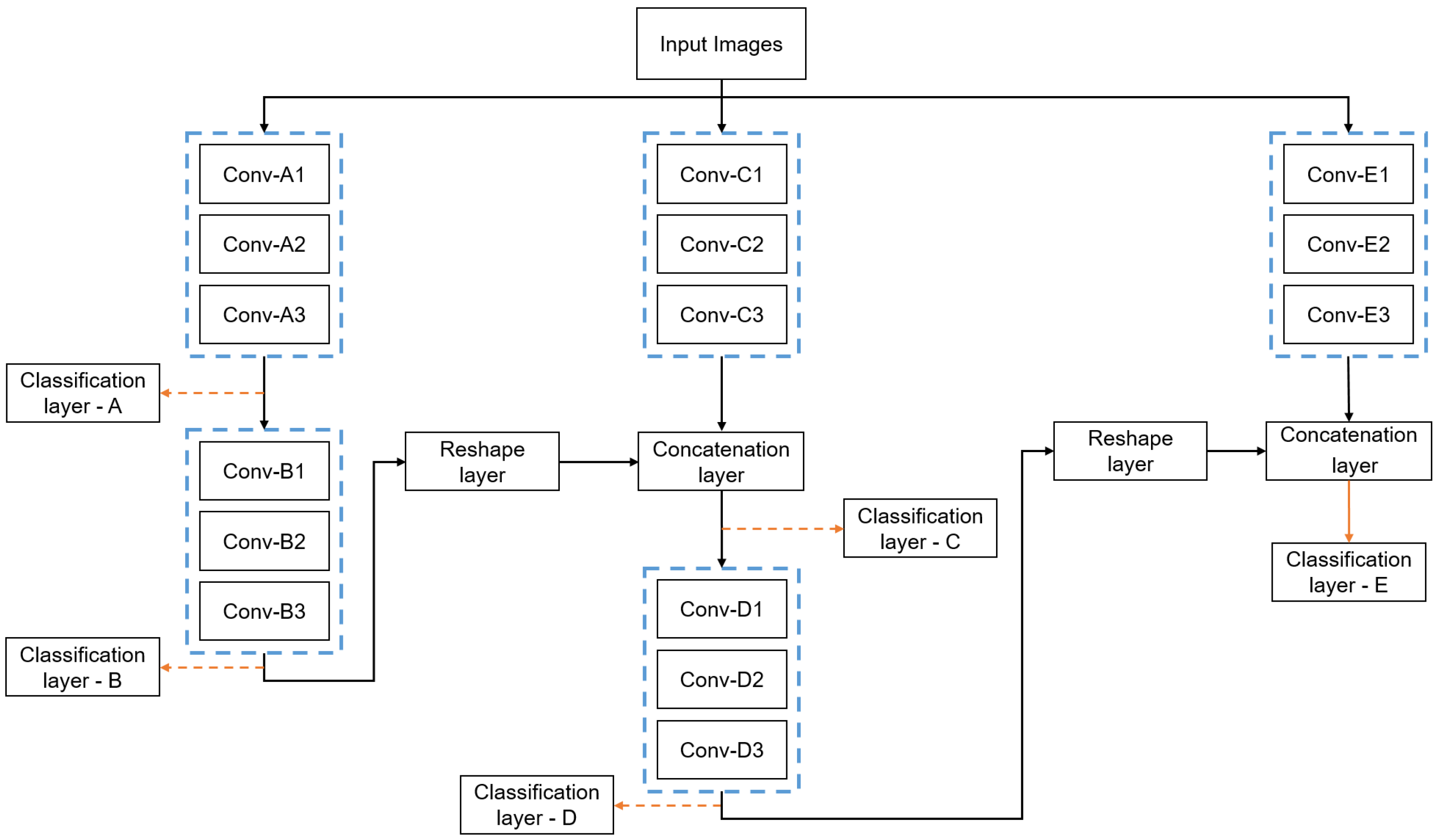
In general, the IMNS can be used to create a limitless number of final architectures by combining the proposed SubNets, or other SubNet architectures. Here, we propose one specific example that we believe effectively balances performance and computational complexity for the medical imaging applications mentioned in Section 1. The proposed IMNet architecture is illustrated in Figure 9. Figure 9 shows five SubNets, A, B, C, D, and E, that are incrementally added to produce the final network. We use relatively small and compact SubNet modules to maintain a small computational cost. The details for each SubNet are provided in Table 2. Figure 7a shows the workflow for adding the SubNet in series, and Figure 7b shows the addition of a parallel SubNet.
First, we use all of the available minibatches to train the SubNet A and minimize the loss to obtain the optimum parameters using Equation (10). After training for SubNet A is complete, we lock in the learnable parameters for this module and refer to it as IMNet A. This network is used to generate the feature maps that will be the input to the new SubNet B. The first convolutional layer of the SubNet B receives all the feature maps from layer of SubNet A as input. In this case, the SubNet B is connected in a series configuration that can be denoted as and we refer to this as IMNet .
Next, we lock the current IMNet , and add a new SubNet C in parallel. This combination of SubNets may be expressed as and we refer to this as IMNet for notational convenience. We use the equations mentioned above to generate feature maps using IMNet and concatenate these with the feature maps generated by the new SubNet C. We use a reshape layer to match the feature map of IMNet with output feature maps of SubNet C and concatenate the feature maps in the depth dimension. SubNet D is then added in series to produce the configuration , denoted here as IMNet . Finally, we lock IMNet and add the last new SubNet E in a parallel configuration. This IMNS sequence can be represented as and we denote this as IMNet . We selected this configuration because we find that alternating between series and parallel SubNets is generally effective, as these two additions tend to complement each other.
3.5. Network Training
We study the performance of our proposed approach by utilizing the following data separation: of the samples of each class are assigned to the training set, to the validation set, and the remaining to the test set. All of the image processing and classification stages are implemented using MATLAB deep learning platform [53] version r2020b. The hardware used is a Windows PC equipped with with Intel Xeon CPU E5-1630 v4 @ GHz and 32 GB of RAM. Network training and testing are accelerated using an NVIDIA TITAN RTX GPU. We trained the network and tuned our hyperparameters for the proposed IMNet architecture solely on the training and validation datasets. All of the IMNets are trained from scratch with randomly initialized weights. We choose the Adam optimization technique [52] to accelerate the convergence time and find the global minimum cost function for all networks. We chose an initial learning rate of with different mini-batch sizes for each application and a validation frequency of 50. Note that the validation frequency details how many iterations pass before re-validating during training. In our configurations we validate every 50 iterations. Note that the learning rate is kept adaptive to accelerate the learning process and prevent over-fitting. The learning rate is scheduled to decrease by a factor of after one half of epochs are completed. We also use a training policy called “ValidationPatience” and set this parameter to 50. This value specifies the number of times that the validation loss can be larger than the smallest value achieved before the training process halts. Furthermore, in order to prevent overfitting and to improve model generalization, we apply a simple and effective regularization technique known as regularization [54] with a value of .
3.6. Statistical Analysis
It is important to assess the efficacy of classification algorithms to aid in method comparisons, method selection, understanding system limitations, and to identify opportunities for future improvement. The metrics we use as performance and efficiency metrics are balanced accuracy (), specificity (), sensitivity (), ROC curves, AUC, and testing time. These metrics defined in [55] provide an objective quantitative picture of the efficacy of the systems tested. We used the two-sided t-test to compare model performances. A was considered statistically significant. All statistical analyses were performed with the statistical package of MATLAB version r2020b. In addition, to test the reproducibility of the model, we repeated such an experiment 10 times and reported mean and standard deviation (SD).
4. Experiment Results
In this section, we present the results obtained using our proposed approaches. In order to demonstrate the efficacy of our proposed algorithm, we compare our IMNS model results against those from well established and state-of-the-art CNN models including AlexNet [56], ResNet [57], Inception v3 [58], DenseNet [59], and NasNet [60]. For these large benchmark networks, we use transfer learning. The weights are imported from MATLAB deep learning toolbox [61] version r2020b. The pre-trained weights are imported from pre-trained networks. The pre-trained networks have been trained on a subset of the ImageNet database [62], which is used in the ILSVRC [44]. Approximately 1.4 million images have been used to train these networks to classify images into 1000 object classes. Fine-tuning a pre-trained network is more efficient than training a network from scratch. This is important with networks of these sizes. For IMNets, we use the training methodology described in Section 3.5. Furthermore, note that our results use publicly available datasets, as described in Section 2, to allow for independently reproducible results. We present the results for our IMNet in several forms to show the evolution in performance using IMNS starting with IMNet A and going to IMNet , as shown in Figure 9. To quantitatively evaluate the results, we employ the performance metrics defined in Section 3.6.
4.1. Quantitative Results Summary
We applied the IMNS method to each of the datasets described in Section 2. In particular, we consider the detection of malaria, DR, and TB. The results for these three experiments are, respectively, summarized in Table 3, Table 4 and Table 5.
Table 3 shows the performance metrics for the IMNS method with various IMNets for malaria detection using blood smear slide images. Note that here IMNet had a significantly higher BACC () than AlexNet, ResNet, DenseNet, and NasNet ( [], [], [], and [], respectively). In addition, our proposed IMNet outperforms the Inception v3 in this experiment ( []). Furthermore, note that IMNet took only seconds to process 5512 samples ( faster than Inception v3). The highest AUC in this experiment is achieved with IMNet . Note also that in this application the addition of SubNet E lowers all of the metrics. This may suggest that the IMNS process can be halted as further improvement is not expected with additional modules.
The results summary for DR detection in retinal images are shown in Table 4. Here the IMNet achieved a higher BACC () which is significantly better than AlexNet and NasNet ( [], and []). The BACC of IMNet is competitive with ResNet, DenseNet and Inception v3 ( [], [], and [], respectively). The DenseNet gives the best BACC here and the ResNet model does have a slightly higher AUC than IMNet . However, IMNet processes 732 images in s, as compared with seconds for ResNet As can be seen by the different IMNet results in Table 4, the BACC score rises with the addition of each SubNet during the IMNS process in this experiment.
The results summary for TB detection in chest radiographs is presented in Table 5. The highest BACC of is achieved with IMNet , which is significantly higher than AlexNet, Inception v3, and NasNet ( [p < 0.05], [], and [], respectively). The IMNet produces a higher BACC than ResNet and DenseNet ( [], and []). The highest AUC of is achieved with IMNet which is significantly higher than the best of benchmark methods, DenseNet, ( []). Note that these IMNets outperform the large scale models in this application with far less computational cost and computational time. Results in Table 5 also indicate a modest but consistent boost in the performance as we add more SubNets during the IMNS process.
Moreover, we compare our IMNets against different current state-of-the-art methods. For malaria application, our IMNet has a comparative AUC score of compared with the current state-of-the-art methods with lower computational complexity, including Rajaraman et al. () [63], Rahman et al. () [28], and Rajaraman et al. () [48]. For DR application, IMNet and IMNet produced a comparable AUC of and relatively lower computational complexity with the following proposed methods, including Gulshan et al. () [64], Chetoui et al. () [38], and Sahlsten et al. () [65]. Finally, IMNet has a comparative AUC score of compared with the following state-of-the-art methods, including Meraj et al. () [66], Sathitratanacheewin et al. () [67], and Hwang et al. () [40].
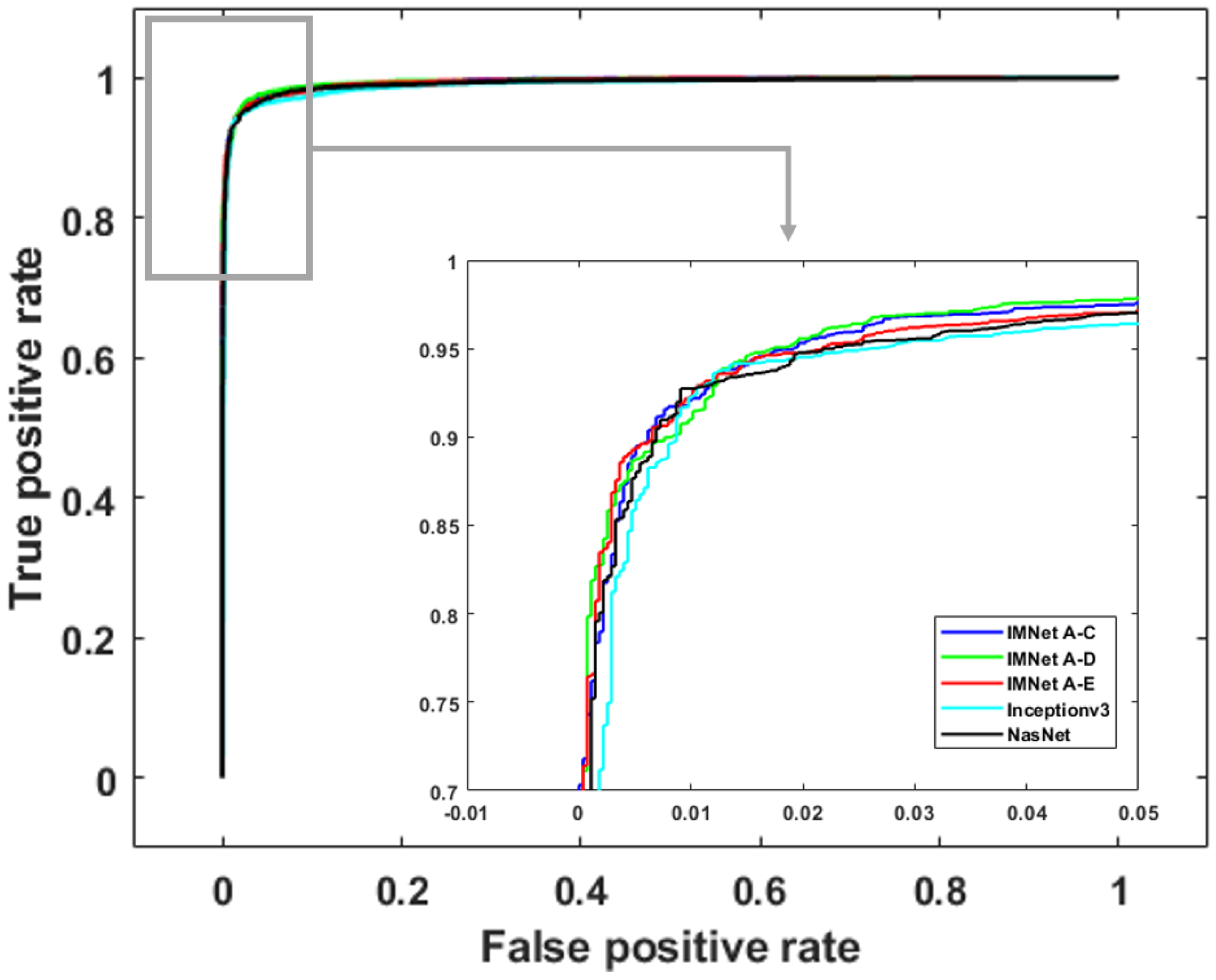
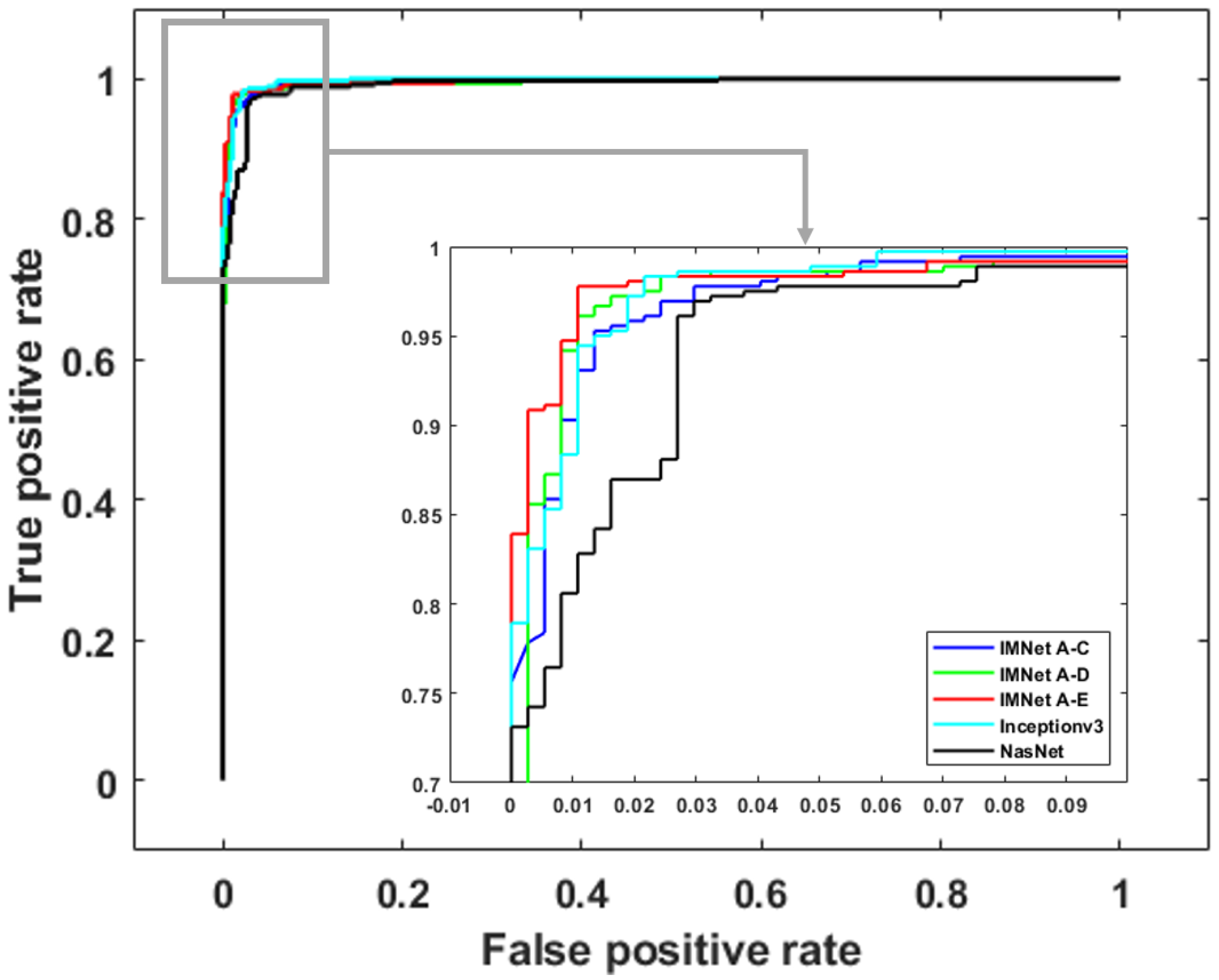
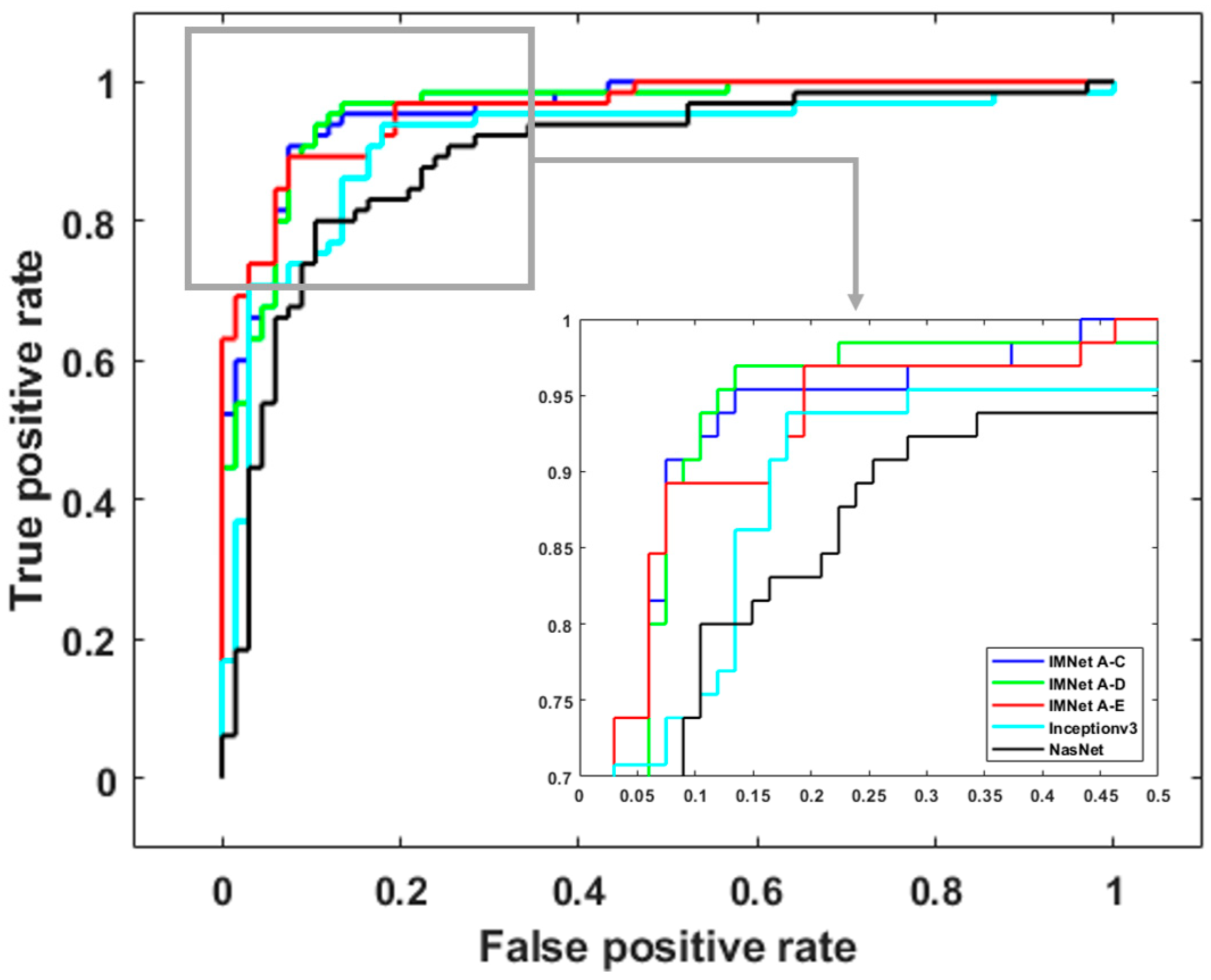
Figure 10, Figure 11 and Figure 12 show ROC curves for malaria, DR, and TB, respectively. The ROC curves provide further insight because they illustrate classifier performance for a range of operating points. For clarity, we only show ROC curves for the top five models in each application. For malaria detection, the IMNet obtained the best result in terms of AUC and an area of . However, IMNet obtained a competitive AUC score for both DR and TB with areas of and , respectively.
4.2. Computational Complexity Comparison
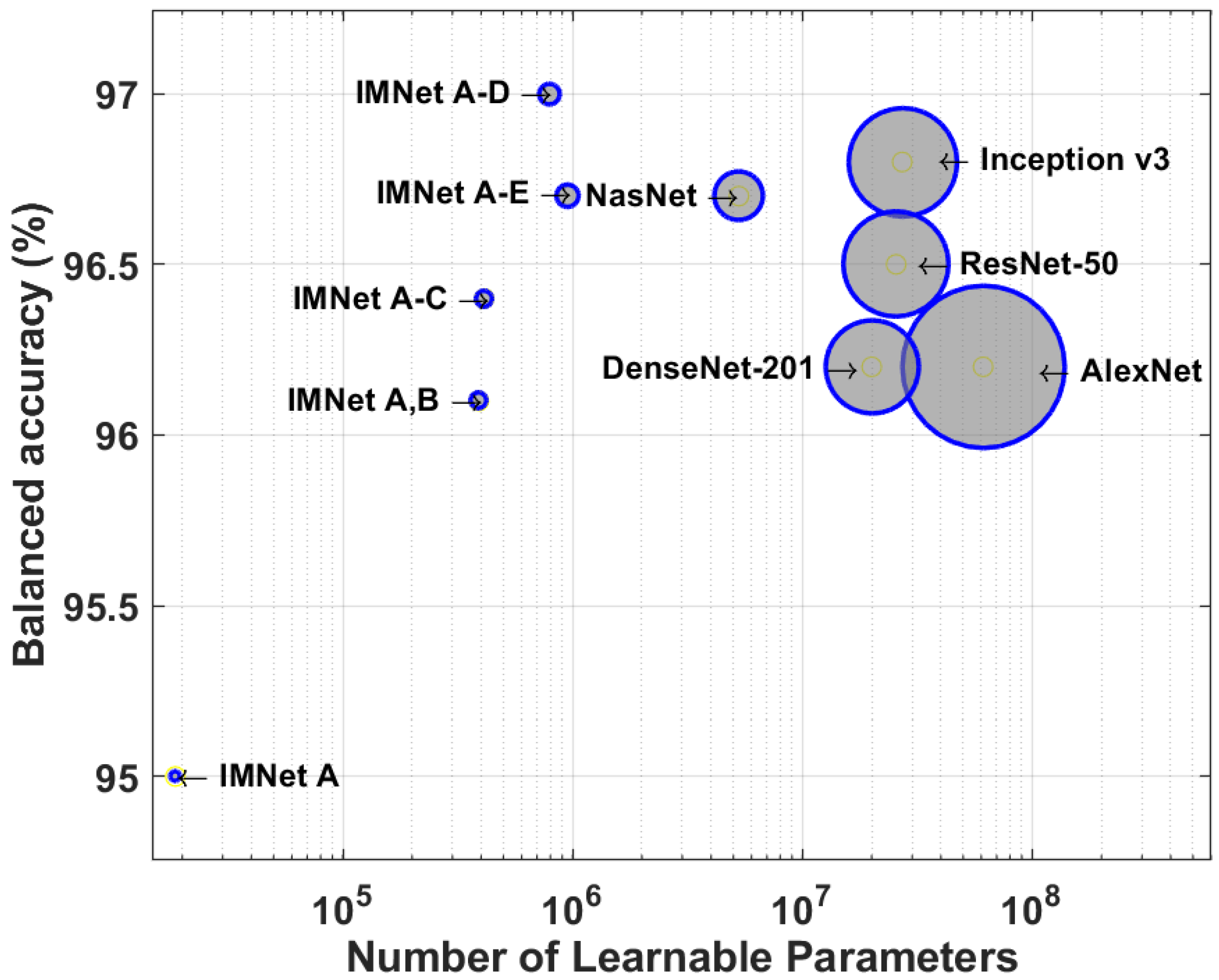
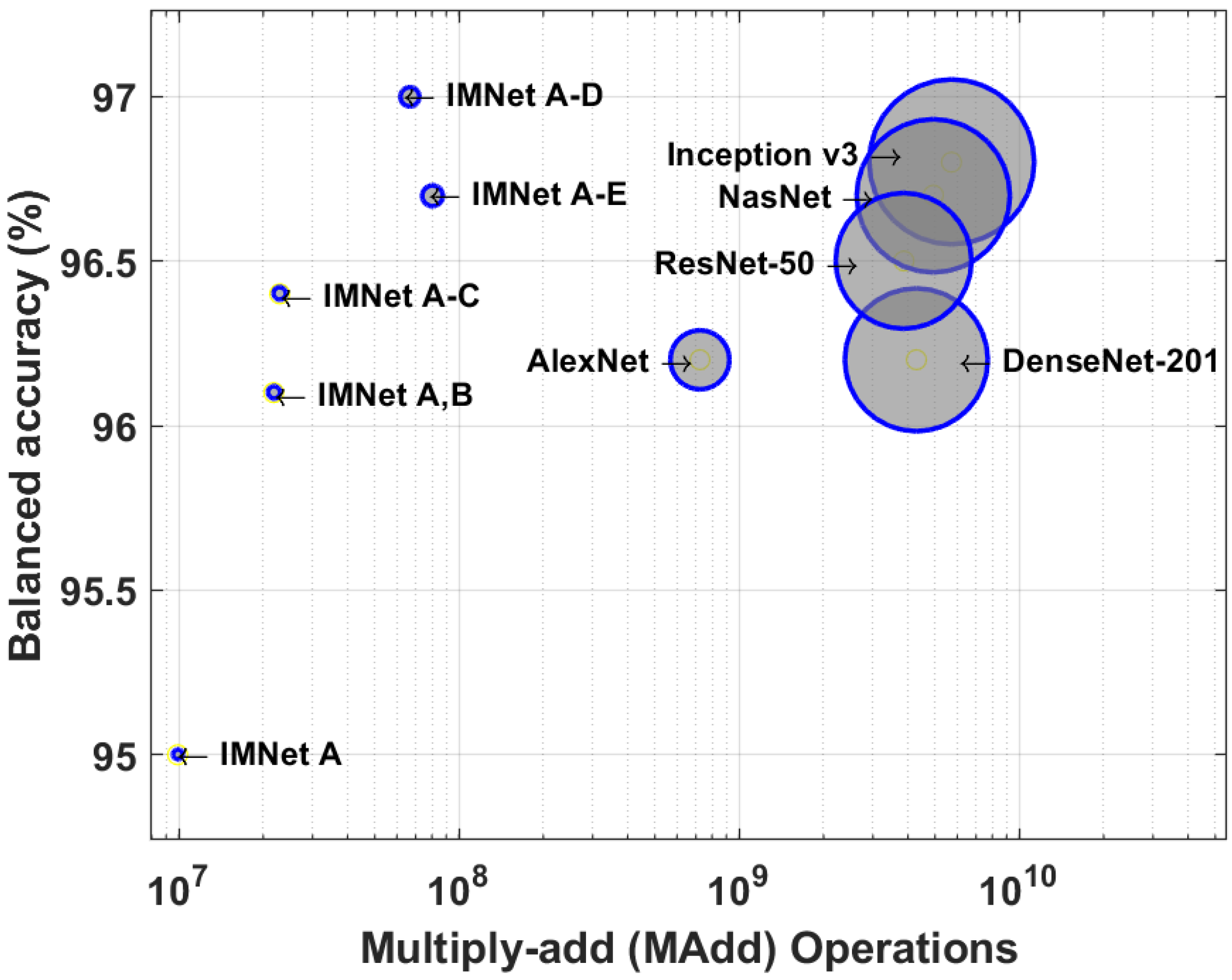
In this section, we compare the computational complexity of AlexNet, ResNet, Inception v3, DenseNet, NasNet, and IMNets by counting the number of multiplications and additions required to process a single image. Furthermore, we compare between all mentioned models the total number of learnable parameters within each CNN model. We calculate the number of learnable parameters for each layer, and then sum up the learnable parameters in each layer to obtain the total amount of learnable parameters in the entire network. Figure 13 and Figure 14 and Table 6 show the results of our computational complexity study. In Figure 13, we show balanced accuracy on the malaria dataset versus the number of learnable parameters. On the other hand, in Figure 13 we show balanced accuracy versus the number of floating-point multiply–add (MAdd) operations for the same dataset. Note that the composite MAdd operations are determined for the input images size of reported in Section 2.1. The diameter of each circle is proportional to the the total number of learnable parameters for Figure 13, and the circle size is the MAdd for Figure 14. Note that the IMNets have fewer learnable parameters, and fewer MAdd operations, as shown in Table 6.
The numerical values for the total number of learnable parameters and MAdd counts are listed in Table 2 for the malaria dataset networks. Note that IMNet (the largest IMNet tested here) has fewer parameters than AlexNet by a factor of approximately 64, and by a factor of approximately 6 compared with NasNet. In terms of the MAdd count, IMNet has fewer than AlexNet by a factor of approximately 9, and fewer than NasNet by a factor of approximately 61.
4.3. Visual Explanations
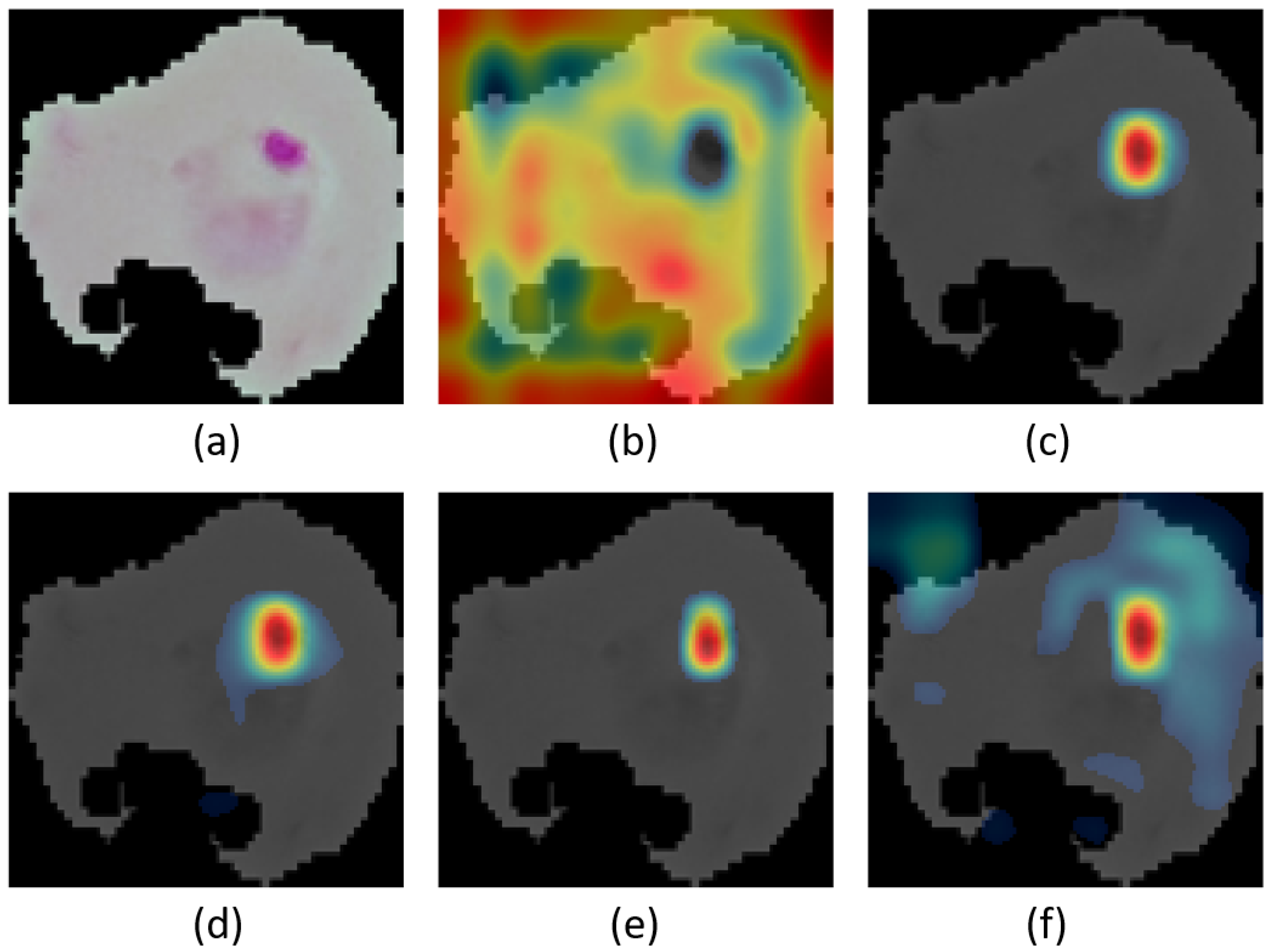
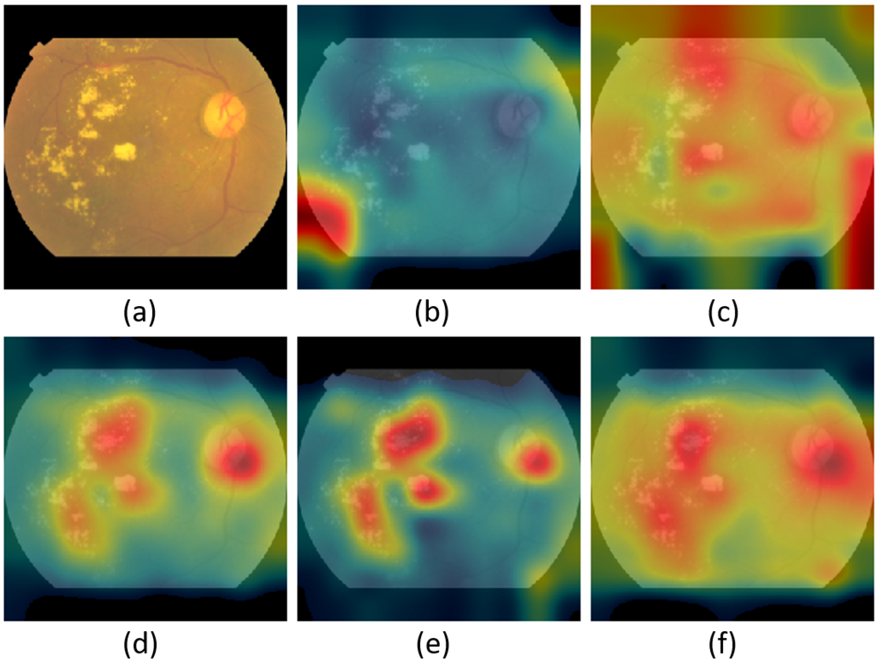
Figure 15, Figure 16 and Figure 17 show the class activation mapping (CAM) [68] outcomes for malaria, DR, and TB, respectively. The examples are for different IMNets on test samples that had been identified as a true positives by the medical professionals. The CAM outputs can give us more confidence in our models’ predictions as they highlight the discriminative regions used by a model to identify a positive class in the dataset. Our goal is to investigate and understand which image region has contributed more to the final model prediction. The idea of the CAM is the following: the probabilities predicted by the network are mapped back to the final convolutional layer to highlight the discriminative regions that are specific to that class [68]. CAM is the output of the activation map after the last convolutional layer for a particular class. CAM is the global average pooling layer applied following the last convolutional layer based on the spatial location in order to generate the weights [68]. Therefore, it allows distinguishing the areas within an image that differentiates the class [68].
Consider the malaria detection CAM results in Figure 15. The original sample image is shown in Figure 15a. The nucleic acids carry three components: parasites, white blood cells, and platelets highlighted in a bluish-purple color [69], as shown in the original sample image. The other images in Figure 15 are CAM results overlaid on the original image for IMNet A through IMNet . Note that the red regions in the CAM images correspond to the spatial regions of most significance to the classifier. In the case of the CAM result for IMNet A, shown in Figure 15b, the attention is distributed and not well focused on the clinically significant portion of the thin smear image. On the other hand, as the IMNS process continues and modules are added, the CAM results do show that attention becomes more focused over the stain on the thin smear example to identify the presence of parasites. The CAM results showing the most focus on the nucleus is IMNet , and this is the best performing IMNet as shown in Table 3.
The CAM results for DR are shown in Figure 16. The input retinal image is shown in Figure 16a. Note that the key aspect of detecting or diagnosing DR is the presence of retinal lesions. There are two main types of lesion defects, white lesions and red lesions. The hard and soft exudates are collectively referred to as white lesions. The red lesions are microaneurysms and hemorrhages [70]. The original image contains hard and soft exudates. We can tell that IMNet , IMNet , and IMNet , focused on these hard and soft exudates that appear as white spots on the original image. Interestingly, these networks also appear to be focusing attention on the optic disk, which is the bright disk in the upper right side of the retinal image. This may be because its color and size resemble that of the large white lesions.
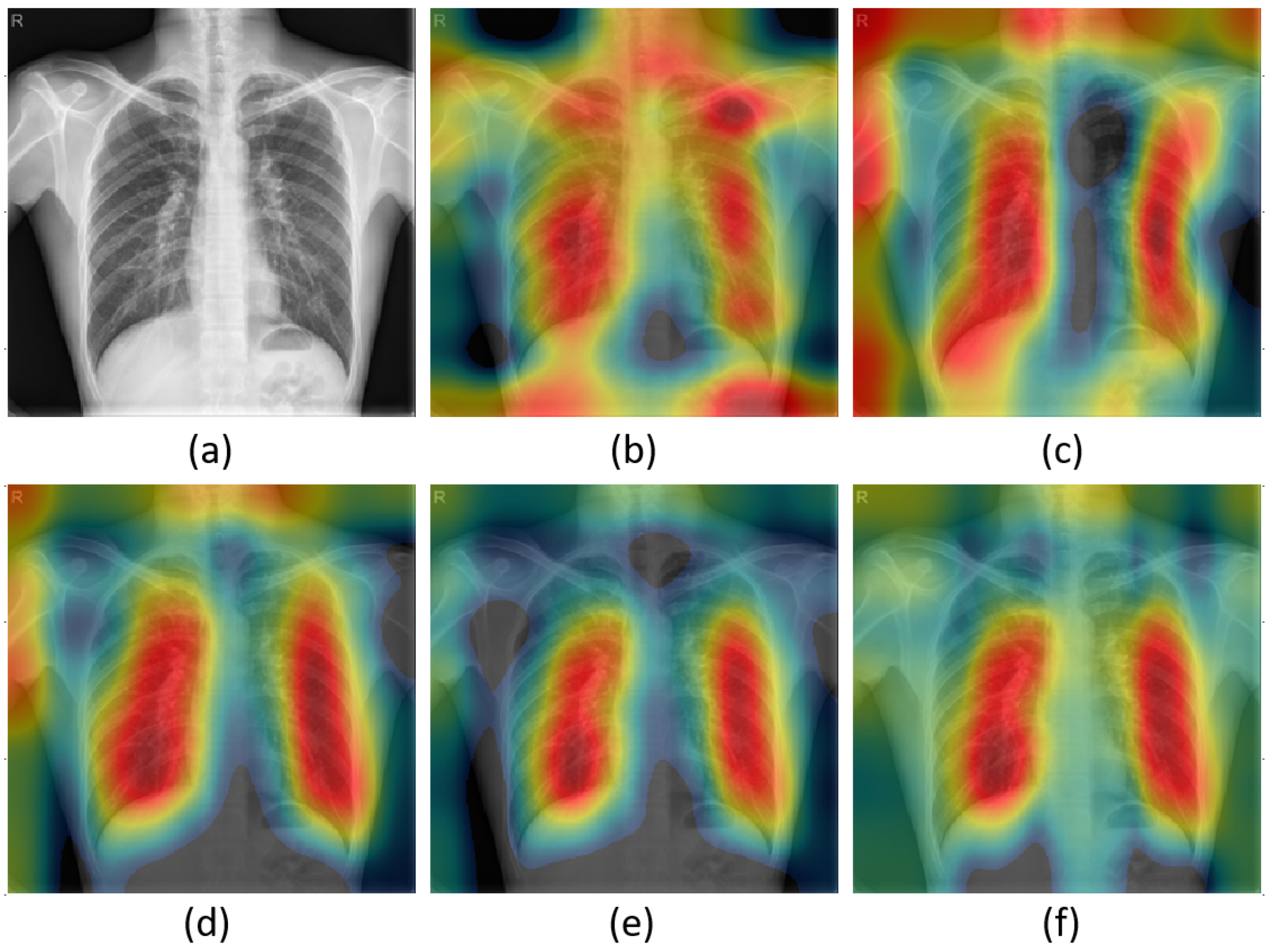
Finally, the CAM for pulmonary tuberculosis is shown in Figure 17. The original CR image with tuberculosis is shown in Figure 17a. Note that there are multiple light areas in the mid-zone lung with fibrotic shadows of primary pulmonary TB. The CAM results for our IMNet models show that attention is focused on these regions. As a result, our model performs well and generally provides an accurate interpretation. Although this example looks good, in many instances, the IMNet A and IMNet CAM results show focus on these clinically significant regions and insignificant regions such as shoulders and background as well. This is consistent with the relatively average classifier performance for that network provided in Table 5. However, all of the other IMNets perform well and tend to produce what we believe are clinically appropriate CAM results.
5. Conclusions and Discussion
In this research, we have proposed IMNS as a new method for designing and training deep learning models. The resulting networks are referred to as IMNets. We have demonstrated the efficacy of the proposed method in detecting three diseases using three different imaging modalities. The best performing IMNets in our study achieved a balanced accuracy of 97.0%, 97.9%, and 88.6% and AUC of 0.995, 0.996, and 0.949 for the detection of malaria, DR, TB, respectively. Our modular approach starts with a single SubNet and we add one additional SubNet at a time, either in series or in parallel with the previous network. Only the new SubNet weights are updated at each stage of IMNS. This approach keeps the computational complexity low and allows the network to train well with a relatively small training set.
The performance of IMNets rivals, and in some cases exceeds, that of much larger state-of-the-art networks where transfer learning is employed. We attribute this to the relatively small training sets available and the limitations of transfer learning. Since the pre-trained networks are trained for a different application, significant adaption may be required for a new task. Large networks can be very powerful where there are sufficient data to properly train them. However, the large networks, with a high number of learnable parameters, can become a liability when only small training sets are available. In other words, for large pre-trained models to be helpful, both extensive data from the same domain and large computational resources are required. It remains the case that large truthed datasets for medical imaging applications are often difficult to come by. This behoves us to explore more compact networks and training strategies such as the proposed IMNS.
Monolithic deep learning with transfer learning may suffer from overfitting issues, due to limited training data in many medical image analysis applications. In addition, the computational cost grows with deeper and wider monolithic networks. The building-block IMNS approach addresses these issues by employing relatively small SubNets and training only one SubNet at a time. As we can see in the results section, our IMNS provides results that rival or exceed many popular large-scale models in the experiments presented here. Moreover, our IMNets trained faster, had lower memory requirements, and processed test images more quickly than the benchmark methods tested.
From a learning perspective, we believe IMNS has several benefits over monolithic deep learning. As with other modular approaches, complex problems are addressed using several small SubNets, rather than one large monolithic network. We believe this helps to mitigate the complex optimization difficulties and vanishing gradient problems that monolithic CNN approaches face. Furthermore, our results suggest that the IMNS allows for the effective transfer of prior knowledge from the fixed portion of the IMNet to a new SubNet. In future work, we plan to extend the architecture of IMNets in two ways. First, we will investigate the impact of combining these SubNets in different configurations. Moreover, we will also examine different SubNet architectures.
Author Contributions
Conceptualization, R.A. and R.C.H.; methodology, R.A. and R.C.H.; software, R.A. and R.C.H.; validation, R.A., R.C.H. and B.N.N.; writing—original draft preparation, R.A.; writing—review and editing, R.A., R.C.H., B.N.N. and T.M.K.; supervision, R.C.H., B.N.N. and T.M.K. All authors have read and agreed to the published version of the manuscript.
Funding
This research received no external funding.
Institutional Review Board Statement
Not applicable.
Informed Consent Statement
Not applicable.
Data Availability Statement
The segmented cells from the thin blood smear slide images for the parasitized and uninfected classes are available at https://lhncbc.nlm.nih.gov/, accessed on 22 May 2022 The publicly available datasets for DR detection can be found at https://www.kaggle.com/competitions/aptos2019-blindness-detection/data, accessed on 22 May 2022 The Shenzhen dataset for TB detection is available at https://lhncbc.nlm.nih.gov/, accessed on 22 May 2022.
Acknowledgments
In no particular order, we thank Vijayan Asari, John S. Loomis and Youssef N. Raffoul for their helpful discussions and suggestions.
Conflicts of Interest
The authors declare that there is no conflict of interest.
References
- Zhai, X.; Kolesnikov, A.; Houlsby, N.; Beyer, L. Scaling vision transformers. arXiv 2021, arXiv:2106.04560. [Google Scholar]
- Riquelme, C.; Puigcerver, J.; Mustafa, B.; Neumann, M.; Jenatton, R.; Pinto, A.S.; Keysers, D.; Houlsby, N. Scaling Vision with Sparse Mixture of Experts. arXiv 2021, arXiv:2106.05974. [Google Scholar]
- Image Classification on ImageNe. Available online: https://paperswithcode.com/sota/image-classification-on-imagenet (accessed on 6 July 2021).
- D’souza, R.N.; Huang, P.Y.; Yeh, F.C. Structural analysis and optimization of convolutional neural networks with a small sample size. Sci. Rep. 2020, 10, 1–13. [Google Scholar] [CrossRef] [PubMed]
- Arsenovic, M.; Karanovic, M.; Sladojevic, S.; Anderla, A.; Stefanovic, D. Solving current limitations of deep learning based approaches for plant disease detection. Symmetry 2019, 11, 939. [Google Scholar] [CrossRef] [Green Version]
- Cremer, C.Z. Deep limitations? Examining expert disagreement over deep learning. Prog. Artif. Intell. 2021, 26, 1–16. [Google Scholar] [CrossRef]
- Lv, X.; Zhang, X. Generating chinese classical landscape paintings based on cycle-consistent adversarial networks. In Proceedings of the 2019 6th International Conference on systems and Informatics (ICSAI), Shanghai, China, 2–4 November 2019; pp. 1265–1269. [Google Scholar]
- Chen, K. Deep and Modular Neural Networks. In Handbook of Computational Intelligence; Springer: Berlin/Heidelberg, Germany, 2015. [Google Scholar]
- Albright, T.D.; Jessell, T.M.; Kandel, E.R.; Posner, M.I. Neural science: A century of progress and the mysteries that remain. Neuron 2000, 25, S1–S55. [Google Scholar] [CrossRef] [Green Version]
- Fodor, J.A. The Modularity of Mind; MIT Press: Cambridge, MA, USA, 1983. [Google Scholar]
- Edelman, G.M. Neural Darwinism: The Theory of Neural Group Selection; Basic Books: New York, NY, USA, 1987. [Google Scholar]
- O’Connell, K.A.; Gatakaa, H.; Poyer, S.; Njogu, J.; Evance, I.; Munroe, E.; Solomon, T.; Goodman, C.; Hanson, K.; Zinsou, C.; et al. Got ACTs? Availability, price, market share and provider knowledge of anti-malarial medicines in public and private sector outlets in six malaria-endemic countries. Malar. J. 2011, 10, 326. [Google Scholar] [CrossRef] [Green Version]
- WHO. World Malaria Report 2020: 20 Years of Global Progress and Challenges; WHO: Geneva, Switzerland, 2020.
- Mace, K.E.; Arguin, P.M.; Tan, K.R. Malaria surveillance—United States, 2015. MMWR Surveill. Summ. 2018, 67, 1. [Google Scholar] [CrossRef]
- Posfai, D.; Sylvester, K.; Reddy, A.; Ganley, J.G.; Wirth, J.; Cullen, Q.E.; Dave, T.; Kato, N.; Dave, S.S.; Derbyshire, E.R. Plasmodium parasite exploits host aquaporin-3 during liver stage malaria infection. PLoS Pathog. 2018, 14, e1007057. [Google Scholar] [CrossRef]
- Dey, N.; Ashour, A.S.; Borra, S. Classification in BioApps: Automation of Decision Making; Springer: Berlin/Heidelberg, Germany, 2017; Volume 26. [Google Scholar]
- WHO. Malaria Microscopy: Quality Assurance Manual, Version 2; WHO: Geneva, Switzerland, 2016.
- Yang, F.; Poostchi, M.; Yu, H.; Zhou, Z.; Silamut, K.; Yu, J.; Maude, R.J.; Jaeger, S.; Antani, S. Deep learning for smartphone-based malaria parasite detection in thick blood smears. IEEE J. Biomed. Health Inform. 2019, 24, 1427–1438. [Google Scholar] [CrossRef]
- Dong, Y.; Jiang, Z.; Shen, H.; Pan, W.D.; Williams, L.A.; Reddy, V.V.; Benjamin, W.H.; Bryan, A.W. Evaluations of deep convolutional neural networks for automatic identification of malaria infected cells. In Proceedings of the 2017 IEEE EMBS International Conference on Biomedical & Health Informatics (BHI), Chicago, IL, USA, 16–19 February 2017; pp. 101–104. [Google Scholar]
- Zheng, Y.; He, M.; Congdon, N. The worldwide epidemic of diabetic retinopathy. Indian J. Ophthalmol. 2012, 60, 428. [Google Scholar] [PubMed]
- Zhang, X.; Wang, H.; Du, C.; Fan, X.; Cui, L.; Chen, H.; Deng, F.; Tong, Q.; He, M.; Yang, M.; et al. Custom-Molded Offloading Footwear Effectively Prevents Recurrence and Amputation, and Lowers Mortality Rates in High-Risk Diabetic Foot Patients: A Multicenter, Prospective Observational Study. Diabetes Metab. Syndr. Obes. Targets Ther. 2022, 15, 103. [Google Scholar] [CrossRef] [PubMed]
- Flaxman, S.R.; Bourne, R.R.; Resnikoff, S.; Ackland, P.; Braithwaite, T.; Cicinelli, M.V.; Das, A.; Jonas, J.B.; Keeffe, J.; Kempen, J.H.; et al. Global causes of blindness and distance vision impairment 1990–2020: A systematic review and meta-analysis. Lancet Glob. Health 2017, 5, e1221–e1234. [Google Scholar] [CrossRef] [Green Version]
- Salz, D.A.; Witkin, A.J. Imaging in diabetic retinopathy. Middle East Afr. J. Ophthalmol. 2015, 22, 145. [Google Scholar] [PubMed]
- Harding, E. WHO global progress report on tuberculosis elimination. Lancet Respir. Med. 2020, 8, 19. [Google Scholar] [CrossRef]
- Narayanan, B.N.; Hardie, R.C.; Krishnaraja, V.; Karam, C.; Davuluru, V.S.P. Transfer-to-transfer learning approach for computer aided detection of COVID-19 in chest radiographs. AI 2020, 1, 539–557. [Google Scholar] [CrossRef]
- World Health Organization. World Malaria Report 2015; World Health Organization: Geneva, Switzerland, 2016.
- Ali, R.; Hardie, R.C.; Ragb, H.K. Ensemble lung segmentation system using deep neural networks. In Proceedings of the 2020 IEEE Applied Imagery Pattern Recognition Workshop (AIPR), Washington, DC, USA, 13–15 October 2020; pp. 1–5. [Google Scholar]
- Rahman, A.; Zunair, H.; Rahman, M.S.; Yuki, J.Q.; Biswas, S.; Alam, M.A.; Alam, N.B.; Mahdy, M. Improving malaria parasite detection from red blood cell using deep convolutional neural networks. arXiv 2019, arXiv:1907.10418. [Google Scholar]
- Pattanaik, P.; Mittal, M.; Khan, M.Z.; Panda, S. Malaria detection using deep residual networks with mobile microscopy. J. King Saud-Univ.-Comput. Inf. Sci. 2022, 34, 1700–1705. [Google Scholar] [CrossRef]
- Zhao, O.S.; Kolluri, N.; Anand, A.; Chu, N.; Bhavaraju, R.; Ojha, A.; Tiku, S.; Nguyen, D.; Chen, R.; Morales, A.; et al. Convolutional neural networks to automate the screening of malaria in low-resource countries. PeerJ 2020, 8, e9674. [Google Scholar] [CrossRef]
- Poostchi, M.; Silamut, K.; Maude, R.J.; Jaeger, S.; Thoma, G. Image analysis and machine learning for detecting malaria. Transl. Res. 2018, 194, 36–55. [Google Scholar] [CrossRef] [Green Version]
- Lee, Y.W.; Choi, J.W.; Shin, E.H. Machine learning model for predicting malaria using clinical information. Comput. Biol. Med. 2020, 129, 104151. [Google Scholar] [CrossRef] [PubMed]
- Narayanan, B.N.; Ali, R.; Hardie, R.C. Performance analysis of machine learning and deep learning architectures for malaria detection on cell images. In Applications of Machine Learning; International Society for Optics and Photonics: Bellingham, WA, USA, 2019; Volume 11139, p. 111390W. [Google Scholar]
- Qummar, S.; Khan, F.G.; Shah, S.; Khan, A.; Shamshirband, S.; Rehman, Z.U.; Khan, I.A.; Jadoon, W. A deep learning ensemble approach for diabetic retinopathy detection. IEEE Access 2019, 7, 150530–150539. [Google Scholar] [CrossRef]
- Zhang, S.; Wu, H.; Murthy, V.; Wang, X.; Cao, L.; Schwartz, J.; Hernandez, J.; Rodriguez, G.; Liu, B.J. The application of deep learning for diabetic retinopathy prescreening in research eye-PACS. In Medical Imaging 2018: Imaging Informatics for Healthcare, Research, and Applications; International Society for Optics and Photonics: Bellingham, WA, USA, 2018; Volume 10579, p. 1057913. [Google Scholar]
- Majumder, S.; Elloumi, Y.; Akil, M.; Kachouri, R.; Kehtarnavaz, N. A deep learning-based smartphone app for real-time detection of five stages of diabetic retinopathy. In Real-Time Image Processing and Deep Learning 2020; International Society for Optics and Photonics: Bellingham, WA, USA, 2020; Volume 11401, p. 1140106. [Google Scholar]
- Narayanan, B.N.; Hardie, R.C.; De Silva, M.S.; Kueterman, N.K. Hybrid machine learning architecture for automated detection and grading of retinal images for diabetic retinopathy. J. Med Imaging 2020, 7, 034501. [Google Scholar] [CrossRef] [PubMed]
- Chetoui, M.; Akhloufi, M.A. Explainable end-to-end deep learning for diabetic retinopathy detection across multiple datasets. J. Med. Imaging 2020, 7, 044503. [Google Scholar] [CrossRef]
- Niazi, M.K.K.; Beamer, G.; Gurcan, M.N. An application of transfer learning to neutrophil cluster detection for tuberculosis: Efficient implementation with nonmetric multidimensional scaling and sampling. In Medical Imaging 2018: Digital Pathology; International Society for Optics and Photonics: Bellingham, WA, USA, 2018; Volume 10581, p. 1058108. [Google Scholar]
- Hwang, S.; Kim, H.E.; Jeong, J.; Kim, H.J. A novel approach for tuberculosis screening based on deep convolutional neural networks. In Medical imaging 2016: Computer-Aided Diagnosis; SPIE: Bellingham, WA, USA, 2016; Volume 9785, pp. 750–757. [Google Scholar]
- Wu, E.Q.; Zhou, M.; Hu, D.; Zhu, L.; Tang, Z.; Qiu, X.Y.; Deng, P.Y.; Zhu, L.M.; Ren, H. Self-Paced Dynamic Infinite Mixture Model for Fatigue Evaluation of Pilots’ Brains. IEEE Trans. Cybern. 2020. [Google Scholar] [CrossRef]
- Panicker, R.O.; Kalmady, K.S.; Rajan, J.; Sabu, M. Automatic detection of tuberculosis bacilli from microscopic sputum smear images using deep learning methods. Biocybern. Biomed. Eng. 2018, 38, 691–699. [Google Scholar] [CrossRef]
- Li, X.; Zhou, Y.; Du, P.; Lang, G.; Xu, M.; Wu, W. A deep learning system that generates quantitative CT reports for diagnosing pulmonary tuberculosis. Appl. Intell. 2021, 51, 4082–4093. [Google Scholar] [CrossRef]
- Russakovsky, O.; Deng, J.; Su, H.; Krause, J.; Satheesh, S.; Ma, S.; Huang, Z.; Karpathy, A.; Khosla, A.; Bernstein, M.; et al. Imagenet large scale visual recognition challenge. Int. J. Comput. Vis. 2015, 115, 211–252. [Google Scholar] [CrossRef] [Green Version]
- Deng, W.; Zhang, X.; Zhou, Y.; Liu, Y.; Zhou, X.; Chen, H.; Zhao, H. An enhanced fast non-dominated solution sorting genetic algorithm for multi-objective problems. Inf. Sci. 2022, 585, 441–453. [Google Scholar] [CrossRef]
- Chen, T.; Goodfellow, I.; Shlens, J. Net2Net: Accelerating Learning via Knowledge Transfer. arXiv 2016, arXiv:1511.05641. [Google Scholar]
- Anderson, A.; Shaffer, K.; Yankov, A.; Corley, C.D.; Hodas, N.O. Beyond Fine Tuning: A Modular Approach to Learning on Small Data. arXiv 2016, arXiv:1611.01714. [Google Scholar]
- Rajaraman, S.; Antani, S.K.; Poostchi, M.; Silamut, K.; Hossain, M.A.; Maude, R.J.; Jaeger, S.; Thoma, G.R. Pre-trained convolutional neural networks as feature extractors toward improved malaria parasite detection in thin blood smear images. PeerJ 2018, 6, e4568. [Google Scholar] [CrossRef] [PubMed]
- APTOS 2019 Blindness Detection. Available online: https://www.kaggle.com/c/aptos2019-blindness-detection/overview (accessed on 14 December 2020).
- Jaeger, S.; Candemir, S.; Antani, S.; Wáng, Y.X.J.; Lu, P.X.; Thoma, G. Two public chest X-ray datasets for computer-aided screening of pulmonary diseases. Quant. Imaging Med. Surg. 2014, 4, 475. [Google Scholar] [PubMed]
- Finlayson, G.D.; Trezzi, E. Shades of gray and colour constancy. In Proceedings of the Color and Imaging Conference. Society for Imaging Science and Technology, Scottsdale, AZ, USA, 9–12 November 2004; Volume 2004, pp. 37–41. [Google Scholar]
- Kingma, D.P.; Ba, J. Adam: A Method for Stochastic Optimization. arXiv 2015, arXiv:1412.6980. [Google Scholar]
- Kim, P. Matlab deep learning. In With Machine Learning, Neural Networks and Artificial Intelligence; Springer: Berkeley, CA, USA, 2017; Volume 130. [Google Scholar]
- Ng, A.Y. Feature selection, L 1 vs. L 2 regularization, and rotational invariance. In Proceedings of the 21st International Conference on Machine Learning, Banff, AB, Canada, 4–8 July 2004; p. 78. [Google Scholar]
- Brinker, T.J.; Hekler, A.; Utikal, J.S.; Grabe, N.; Schadendorf, D.; Klode, J.; Berking, C.; Steeb, T.; Enk, A.H.; Von Kalle, C. Skin cancer classification using convolutional neural networks: Systematic review. J. Med. Internet Res. 2018, 20, e11936. [Google Scholar] [CrossRef]
- Krizhevsky, A.; Sutskever, I.; Hinton, G.E. Imagenet classification with deep convolutional neural networks. Adv. Neural Inf. Process. Syst. 2012, 25, 1097–1105. [Google Scholar] [CrossRef]
- He, K.; Zhang, X.; Ren, S.; Sun, J. Deep residual learning for image recognition. In Proceedings of the IEEE Conference on Computer Vision and Pattern Recognition, Las Vegas, NV, USA, 27–30 June 2016; pp. 770–778. [Google Scholar]
- Szegedy, C.; Vanhoucke, V.; Ioffe, S.; Shlens, J.; Wojna, Z. Rethinking the inception architecture for computer vision. In Proceedings of the IEEE Conference on Computer Vision and Pattern Recognition, New York, NY, USA, 17–22 June 2016; pp. 2818–2826. [Google Scholar]
- Huang, G.; Liu, Z.; Van Der Maaten, L.; Weinberger, K.Q. Densely connected convolutional networks. In Proceedings of the IEEE Conference on Computer Vision and Pattern Recognition, Honolulu, HI, USA, 21–26 July 2017; pp. 4700–4708. [Google Scholar]
- Zoph, B.; Vasudevan, V.; Shlens, J.; Le, Q.V. Learning transferable architectures for scalable image recognition. In Proceedings of the IEEE Conference on Computer Vision and Pattern Recognition, Salt Lake City, UT, USA, 18–23 June 2018; pp. 8697–8710. [Google Scholar]
- MATLAB Deep Learning Toolbox Documentation. Available online: https://www.mathworks.com/help/deeplearning/ (accessed on 6 July 2021).
- Deng, J.; Dong, W.; Socher, R.; Li, L.J.; Li, K.; Fei-Fei, L. Imagenet: A large-scale hierarchical image database. In Proceedings of the 2009 IEEE Conference on Computer Vision and Pattern Recognition, Miami, FL, USA, 20–25 June 2009; pp. 248–255. [Google Scholar]
- Rajaraman, S.; Jaeger, S.; Antani, S.K. Performance evaluation of deep neural ensembles toward malaria parasite detection in thin-blood smear images. PeerJ 2019, 7, e6977. [Google Scholar] [CrossRef] [Green Version]
- Gulshan, V.; Peng, L.; Coram, M.; Stumpe, M.C.; Wu, D.; Narayanaswamy, A.; Venugopalan, S.; Widner, K.; Madams, T.; Cuadros, J.; et al. Development and validation of a deep learning algorithm for detection of diabetic retinopathy in retinal fundus photographs. JAMA 2016, 316, 2402–2410. [Google Scholar] [CrossRef]
- Sahlsten, J.; Jaskari, J.; Kivinen, J.; Turunen, L.; Jaanio, E.; Hietala, K.; Kaski, K. Deep learning fundus image analysis for diabetic retinopathy and macular edema grading. Sci. Rep. 2019, 9, 1–11. [Google Scholar] [CrossRef] [Green Version]
- Meraj, S.S.; Yaakob, R.; Azman, A.; Rum, S.; Shahrel, A.; Nazri, A.; Zakaria, N.F. Detection of pulmonary tuberculosis manifestation in chest X-rays using different convolutional neural network (CNN) models. Int. J. Eng. Adv. Technol. (IJEAT) 2019, 9, 2270–2275. [Google Scholar] [CrossRef]
- Sathitratanacheewin, S.; Sunanta, P.; Pongpirul, K. Deep learning for automated classification of tuberculosis-related chest X-Ray: Dataset distribution shift limits diagnostic performance generalizability. Heliyon 2020, 6, e04614. [Google Scholar] [CrossRef] [PubMed]
- Zhou, B.; Khosla, A.; Lapedriza, A.; Oliva, A.; Torralba, A. Learning deep features for discriminative localization. In Proceedings of the IEEE Conference on Computer Vision and Pattern Recognition, Las Vegas, NV, USA, 27–30 June 2016; pp. 2921–2929. [Google Scholar]
- Prasad, K.; Winter, J.; Bhat, U.M.; Acharya, R.V.; Prabhu, G.K. Image analysis approach for development of a decision support system for detection of malaria parasites in thin blood smear images. J. Digit. Imaging 2012, 25, 542–549. [Google Scholar] [CrossRef] [PubMed] [Green Version]
- Borsos, B.; Nagy, L.; Iclanzan, D.; Szilágyi, L. Automatic detection of hard and soft exudates from retinal fundus images. Acta Unitiversitatis-Sapientiae-Inform. 2019, 11, 65–79. [Google Scholar] [CrossRef] [Green Version]
Figure 1.
Raw parasitized and uninfected sample images for malaria detection labeled by expert slide readers.
Figure 1.
Raw parasitized and uninfected sample images for malaria detection labeled by expert slide readers.

Figure 2.
Malaria detection images from Figure 1 after color constancy processing.
Figure 2.
Malaria detection images from Figure 1 after color constancy processing.

Figure 3.
Raw retinal images of a healthy retina (normal class) and DR damage blood vessels in the retina (DR class).
Figure 3.
Raw retinal images of a healthy retina (normal class) and DR damage blood vessels in the retina (DR class).

Figure 4.
Retinal images from Figure 3 after applying the proposed pre-processing steps to normalize the images in the database.
Figure 4.
Retinal images from Figure 3 after applying the proposed pre-processing steps to normalize the images in the database.

Figure 5.
Chest radiograph samples from the Shenzhen dataset labeled by radiologists as normal and tuberculosis. Starting from the left, the first, second, and fourth chest radiograph images have inverse polarity.
Figure 5.
Chest radiograph samples from the Shenzhen dataset labeled by radiologists as normal and tuberculosis. Starting from the left, the first, second, and fourth chest radiograph images have inverse polarity.

Figure 6.
Preprocessed chest radiograph images from the Shenzhen dataset to provide polarity uniformity.
Figure 6.
Preprocessed chest radiograph images from the Shenzhen dataset to provide polarity uniformity.

Figure 7.
Illustration of the IMNS workflow for building IMNets. (a) Addition of a series SubNet, (b) addition of a parallel SubNet.
Figure 7.
Illustration of the IMNS workflow for building IMNets. (a) Addition of a series SubNet, (b) addition of a parallel SubNet.

Figure 8.
(a) Convolutional layer structure. (b) Classification layer structure.

Figure 9.
IMNet architecture used here in the experimental results. SubNets A, B, C, D and E are added incrementally in order to produce the full network shown. Details of the SubNets are provided in Table 2.
Figure 9.
IMNet architecture used here in the experimental results. SubNets A, B, C, D and E are added incrementally in order to produce the full network shown. Details of the SubNets are provided in Table 2.

Figure 10.
Malaria dataset ROC curve for the five best performing networks.

Figure 11.
Diabetic retinopathy dataset ROC curve for the five best performing networks.

Figure 12.
Tuberculosis dataset ROC curve for the five best performing networks.

Figure 13.
Balanced accuracy on the malaria dataset versus the number of learnable parameters. The computational cost is measured based on the number of MAdd operations to process a single example. The diameter of each circle is proportional to the total number of learnable parameters of the network.

Figure 14.
Balanced accuracy on the malaria dataset versus the number of floating-point multiply–add (MAdd) operations. The computational cost is measured based on the number of MAdd operations to process a single example. The diameter of each circle is proportional to the MAdd of the network.
Figure 14.
Balanced accuracy on the malaria dataset versus the number of floating-point multiply–add (MAdd) operations. The computational cost is measured based on the number of MAdd operations to process a single example. The diameter of each circle is proportional to the MAdd of the network.

Figure 15.
CAM visualization on malaria dataset for a test sample using various IMNets: (a) Original sample, (b) IMNet (c) IMNet , (d) IMNet , (e) IMNet , and (f) IMNet .
Figure 15.
CAM visualization on malaria dataset for a test sample using various IMNets: (a) Original sample, (b) IMNet (c) IMNet , (d) IMNet , (e) IMNet , and (f) IMNet .

Figure 16.
CAM visualization on DR dataset for a test sample using various IMNets: (a) Original sample, (b) IMNet (c) IMNet , (d) IMNet , (e) IMNet , and (f) IMNet .
Figure 16.
CAM visualization on DR dataset for a test sample using various IMNets: (a) Original sample, (b) IMNet (c) IMNet , (d) IMNet , (e) IMNet , and (f) IMNet .

Figure 17.
CAM visualization on TB dataset for a test sample using various IMNets: (a) Original sample, (b) IMNet (c) IMNet , (d) IMNet , (e) IMNet , and (f) IMNet .
Figure 17.
CAM visualization on TB dataset for a test sample using various IMNets: (a) Original sample, (b) IMNet (c) IMNet , (d) IMNet , (e) IMNet , and (f) IMNet .


Table 1.
The hold-out validation distribution of the data source for each application and the number of training, validation, and testing cases.
Table 1.
The hold-out validation distribution of the data source for each application and the number of training, validation, and testing cases.
| Applications | Malaria | Diabetic Retinopathy | Tuberculosis | |
|---|---|---|---|---|
| Datasets | ||||
| Images size | ||||
| No. of training set | 19842 | 2637 | 477 | |
| No. of validation set | 2204 | 293 | 53 | |
| No. of testing set | 5512 | 732 | 132 | |
Table 2.
SubNet architectures used in the IMNet in Figure 9.
Table 2.
SubNet architectures used in the IMNet in Figure 9.
| Model | Layers | Filter Size | Total Parameters | MAdd |
|---|---|---|---|---|
| SubNet A | Conv-A2 | 0.018M | 9.94M | |
| Conv-A2 | ||||
| Conv-A3 | ||||
| SubNet B | Conv-B1 | 0.390M | 11.94M | |
| Conv-B2 | ||||
| Conv-B3 | ||||
| SubNet C | Conv-C1 | 0.021M | 1.10M | |
| Conv-C2 | ||||
| Conv-C3 | ||||
| SubNet D | Conv-D1 | 0.390M | 43.65M | |
| Conv-D2 | ||||
| Conv-D3 | ||||
| SubNet E | Conv-E1 | 0.165M | 13.82M | |
| Conv-E2 | ||||
| Conv-E3 |
Table 3.
Malaria dataset results showing hold-out validation performance on the test set using our IMNS method and benchmark methods.
Table 3.
Malaria dataset results showing hold-out validation performance on the test set using our IMNS method and benchmark methods.
| Model | BACC (%) | SPEC (%) | SENS (%) | AUC | Testing Time (s) |
|---|---|---|---|---|---|
| AlexNet | |||||
| ResNet | |||||
| DenseNet | |||||
| Inception v3 | |||||
| NasNet | |||||
| IMNet A | |||||
| IMNet | |||||
| IMNet | |||||
| IMNet | |||||
| IMNet |
Table 4.
Diabetic retinopathy dataset results showing hold-out validation performance on the test set using our IMNS method and benchmark methods.
Table 4.
Diabetic retinopathy dataset results showing hold-out validation performance on the test set using our IMNS method and benchmark methods.
| Model | BACC (%) | SPEC (%) | SENS (%) | AUC | Testing Time (s) |
|---|---|---|---|---|---|
| AlexNet | |||||
| ResNet | |||||
| DenseNet | |||||
| Inception v3 | |||||
| NasNet | |||||
| IMNet A | |||||
| IMNet | |||||
| IMNet | |||||
| IMNet | |||||
| IMNet |
Table 5.
Tuberculosis dataset results showing hold-out validation performance on the test set using our IMNS method and benchmark methods.
Table 5.
Tuberculosis dataset results showing hold-out validation performance on the test set using our IMNS method and benchmark methods.
| Model | BACC (%) | SPEC (%) | SENS (%) | AUC | Testing Time (s) |
|---|---|---|---|---|---|
| AlexNet | |||||
| ResNet | |||||
| DenseNet | |||||
| Inception v3 | |||||
| NasNet | |||||
| IMNet A | |||||
| IMNet | |||||
| IMNet | |||||
| IMNet | |||||
| IMNet |
Table 6.
Resource usage for IMNets in comparison to benchmark models for the malaria dataset networks.
Table 6.
Resource usage for IMNets in comparison to benchmark models for the malaria dataset networks.
| Model | Total Parameters | MAdd |
|---|---|---|
| AlexNet | 61.10M | 0.72G |
| ResNet | 25.56M | 3.87G |
| Inception v3 | 27.16M | 5.72G |
| DenseNet | 20.01M | 4.29G |
| NasNet | 5.290M | 4.93G |
| IMNet A | 0.018M | 0.0099G |
| IMNet | 0.390M | 0.0218G |
| IMNet | 0.412M | 0.0229G |
| IMNet | 0.790M | 0.0666G |
| IMNet | 0.955M | 0.0804G |
Publisher’s Note: MDPI stays neutral with regard to jurisdictional claims in published maps and institutional affiliations. |
© 2022 by the authors. Licensee MDPI, Basel, Switzerland. This article is an open access article distributed under the terms and conditions of the Creative Commons Attribution (CC BY) license (https://creativecommons.org/licenses/by/4.0/).
Share and Cite
MDPI and ACS Style
Ali, R.; Hardie, R.C.; Narayanan, B.N.; Kebede, T.M. IMNets: Deep Learning Using an Incremental Modular Network Synthesis Approach for Medical Imaging Applications. Appl. Sci. 2022, 12, 5500. https://doi.org/10.3390/app12115500
AMA Style
Ali R, Hardie RC, Narayanan BN, Kebede TM. IMNets: Deep Learning Using an Incremental Modular Network Synthesis Approach for Medical Imaging Applications. Applied Sciences. 2022; 12(11):5500. https://doi.org/10.3390/app12115500
Chicago/Turabian StyleAli, Redha, Russell C. Hardie, Barath Narayanan Narayanan, and Temesguen M. Kebede. 2022. "IMNets: Deep Learning Using an Incremental Modular Network Synthesis Approach for Medical Imaging Applications" Applied Sciences 12, no. 11: 5500. https://doi.org/10.3390/app12115500
Note that from the first issue of 2016, this journal uses article numbers instead of page numbers. See further details here.