Indoor Genetic Algorithm-Based 5G Network Planning Using a Machine Learning Model for Path Loss Estimation

Abstract

Accurate wireless network planning is crucial for the deployment of new wireless services. This usually requires the consecutive evaluation of many candidate solutions, which is only feasible for simple path loss models, such as one-slope models or multi-wall models. However, such path loss models are quite straightforward and often do not deliver satisfactory estimations, eventually impacting the quality of the proposed network deployment. More advanced models, such as Indoor Dominant Path Loss models, are usually more accurate, but as their path loss calculation is much more time-consuming, it is no longer possible to evaluate a large set of candidate deployment solutions. Out of necessity, a heuristic network planning algorithm is then typically used, but the outcomes heavily depend on the quality of the heuristic. Therefore, this paper investigates the use of Machine Learning to approximate a complex 5G path loss model. The much lower calculation time allows using this model in a Genetic Algorithm-based network planning algorithm. The Machine Learning model is trained for two buildings and is validated on three other buildings, with a Mean Absolute Error below 3 dB. It is shown that the new approach is able to find a wireless network deployment solution with an equal, or smaller, amount of access points, while still providing the required coverage for at least 99.4% of the receiver locations and it does this 15 times faster. Unlike a heuristic approach, the proposed one also allows accounting for additional design criteria, such as maximal average received power throughout the building, or minimal exposure to radiofrequency signals in certain rooms.

1. Introduction

Fifth Generation (5G) cellular networks are promising to be a real improvement compared to all the previous mobile generation networks [1]. They bring three main services for end-users i.e., Extreme Mobile Broadband (eMBB), Massive Machine Type Communications (eMTC), and Ultra-Reliable Low Latency Communication (URLLC) [1,2]. The 5G New Radio (5G-NR) operates over two frequency ranges: Frequency Range 1 (FR1 includes sub-6 GHz), and Frequency Range 2 (FR2, which includes the millimeter-wave band, from 24.25 to 52.6 GHz). A significant number of commercial 5G networks are currently under deployment in the sub-6 GHz band, particularly in the 3.3–3.8 GHz (3.5 GHz band) portion, which offers a good trade-off between coverage and capacity [3]. Therefore, understanding signal propagation characteristics in the 3.5 GHz band is particularly important, especially in 5G indoor scenarios, where many applications are being developed.

Some 5G use cases target indoor scenarios, such as smart building monitoring with different types of sensors, factory automation, object tracking inside a building, and automated vehicles (logistic applications) [4,5]. These indoor scenarios are likely to be addressed via an outdoor (outdoor-to-indoor, O2I) deployment of the 5G Base Station (BS) [6,7,8]. However, it was demonstrated in [9] that the PL for O2I increases by approximately 100 dB when the distance between the BS and the building is increased by 50 m, and the use of indoor-to-indoor (I2I) deployments can reduce the PL up to 60 dB, compared to O2I deployments. This emphasizes the need for understanding propagation characteristics in indoor scenarios with I2I deployments.

Wireless network planning and optimization are indispensable in modern wireless communication systems, considering the ever-increasing number of Radio Frequency (RF) devices in our daily lives. This usually requires the evaluation of many candidate solutions to find the best system settings and to meet the Quality of Service (QoS) requirements. This is only feasible for simple Path Loss (PL) models, such as one-slope or multi-wall models. These are easy to construct, but their validity is limited to the propagation environment they represent. Furthermore, the estimation of the propagation PL in indoor scenarios is not trivial, due to the complexity and variabilities of the environment. Other approaches are to calculate PL using deterministic models, for example using ray-tracing [10,11], or using a heuristic approach [12]. Deterministic propagation path loss models could provide more accurate estimations of the PL, but they are time-consuming. When calculating one candidate network deployment takes too long, it is unlikely that a wireless network planning algorithm will converge to an optimal solution, i.e., providing coverage with a minimal number of access points. Hence, these complex PL models, despite being more accurate, are less suited to use in the optimal network design process. Alternatively, PL estimations using Machine Learning (ML) techniques are efficient, consume little time, and can be adjusted to fit any environment or propagation condition. As such, these models allow the evaluation of a large number of candidate network deployments when performing network planning, which should eventually lead to an optimal network deployment, that, at the same time, builds on an accurate path loss model.

In this research work, we propose a generic method based on the Decision Tree Ensembles (Bagging) algorithm for the estimation of the PL experienced by 5G signals at 3.5 GHz in indoor scenarios. Subsequently, the obtained model is used in a Genetic Algorithm (GA) [13] to perform 5G network planning. The novelty of this work is (i) to build a generic (applicable to other buildings) ML model able to accurately approximate an advanced PL model, (ii) use the ML estimation in combination with a GA for wireless network planning, and (iii) obtain deployment solutions with similar, or better, performance than existing heuristic tools (e.g., the one developed in [12]), but in less time.

We show that an advanced, but computationally expensive, path loss model, that builds on the physical properties of propagation, can be well approximated by a ML-based PL model that allows much faster PL estimations for a given link. Such a quick, but still accurate, PL model unlocks the possibility of more thorough exploration of the optimization space to find the optimal network deployment (number and location of APs). It is shown that the proposed approach is accurate (i.e., is able to provide the required coverage, according to the complex PL model), is 15 times faster than a heuristic optimization algorithm (and, thus, more flexible towards recalculations with adjusted optimization settings), finds a better solution (with fewer APs), and allows accounting for additional constraints, such as striving for maximal received power.

The remainder of this paper is organized as follows. Section 2 discusses related works on PL estimation and network optimization approaches. Section 3 describes the scenarios in which our generic model is designed, the method used to estimate the PL, and describes the principles of a GA to optimize network deployment. Section 4 describes the performance of PL estimation using the ML algorithm. Also, we investigate the quality of the resulting network planning solution, by comparing the results obtained with an existing heuristic tool in terms of the number of APs, the time to make the planning, and the coverage percentage of the ML-GA-based network design. Finally, Section 5 presents the conclusions of this research.

2. Related Work

2.1. Machine Learning for Path Loss Estimation

The use of ML to solve outdoor/indoor problems in modern communication systems is a topic under research. In [14], the authors presented an overview of the principles and procedure of ML-based PL prediction. To support the research, they used measured data and evaluated the performance of different models, such as Artificial Neural Networks (ANN), Support Vector Regression (SVR), and random forest. In the research, it was proven that ML models outperform the traditional log-distance model.

For indoor scenarios, several research works have been conducted [15,16,17,18]. In [15], the authors proposed a method based on Neural Networks (NN) to estimate the radio frequency exposure generated by Wi-Fi sources in indoor scenarios. As inputs, they used easily measured variables, such as the position and type of Wi-Fi sources and the position and materials of the walls. The NN achieved a Root Mean Squared Error (RMSE) of 2.1–7.0 dB compared to the target electric field obtained with a deterministic indoor network planner. The results show that the solution is comparable to other ML solutions in the same scenario, but the performance was not validated in other buildings. To reduce this lack, in our work we evaluate five different buildings.

A method to automatically construct and optimize a model-based radio map was proposed in [16]. It was based on unsupervised learning, where random walks, for which the ground truth locations are unknown, serve as input for the optimization, along with a floor plan and a location tracking algorithm. Experiments in large office buildings resulted in median accuracy of up to 2 m. In [17], the authors proposed a Convolutional Neural Network (CNN)-based indoor path loss modeling approach. Based on a floor plan and measurement data, input images were generated for training a CNN, which can make predictions of Received Signal Strength of 5 GHz Wi-Fi in an indoor usage scenario. Experiment results showed that CNNs can be used for indoor path loss modeling with encouraging performance from the RMSE of 3.9 dB in the training process. In the test process (only one building was considered) the absolute error of Received Signal Strength (RSS) estimation is within 2 dB for 38% of locations, and within 5 dB for 79% of locations. In our work, we set the coverage condition for the 100% of points in the area of interest.

In [19], the authors proposed a deep learning-based path loss modeling method for 5.8 GHz Wi-Fi, based on a floor plan of a building. It was used for a local area multiple-line scanning (LAMS) algorithm to generate the training dataset. In the end, the model’s performance was compared to real measurements and the 3D ray-tracing method. It was shown that the performance of the model (RMSE = 3.94 dB) compared to real measurements was better than the performance of the ray-tracing method (RMSE = 5.8 dB). The main constraint is related to the use of this model in different scenarios. Since the authors used a LAMS algorithm, using the model in another building requires generating new data and retraining the model. The solution proposed in our work does not need to train the model for use in new buildings, as long as the type fits the specifications. In [20], the authors proposed a path loss model for an Unmanned Aerial Vehicle (UAV) air-to-air (AA) scenario based on ML. Two ML algorithms (K nearest neighbors (kNN) and Random Forest) were used to build the models and the results were compared to the data generated by the ray-tracing software developed in [20]. Both ML models have better performance than the empirical models (COST231 and SUI model), and the Random Forest algorithm even outperforms the kNN by 2 dB. The calculation times for Random Forest and kNN to make predictions are 8.71 s and 5.95 s, respectively. However, running the ray-tracing software took more than 10 min. In [21], the authors compared three ML algorithms: kNN, SVR, and Random Forest. In this case, to avoid time consumption and expensive measurement campaigns, the PL values to train/validate the ML algorithms were generated with a 3D ray-tracing model in the city center of Tripoli, Greece. As a result, they obtained estimations with a Mean Absolute Error (MAE) less than 3 dB for the three ML algorithms, which prove that ML can be both a fast and accurate approach to approximate complex PL models (e.g., ray-tracing). Looking for further improvements, we use in our research the Ensembles trees: the Bagging algorithm, which is a combination of Random Forest algorithm and the Bagging technique to reduce the standard deviation of the error (we refer the reader to Section 3.1.2). Further, we unlock the opportunities that such a quick ML-based PL model brings. Wireless network planning using (ML-approximated) advanced PL models is made possible, allowing for better results and more flexibility in the planning process.

2.2. Network Planning Algorithms

To ensure the best network connectivity to users, wireless network planning is of utmost importance. Rational planning (i.e., minimizing the number of APs) and effective planning of the wireless network (i.e., maximizing the throughput) for indoor/outdoor operation usually requires the consecutive evaluation of many candidate solutions using optimization algorithms. Among the optimization algorithms commonly used in network planning, we can mention: e.g., heuristics [12,22,23,24], GA [25,26,27,28], or Particle Swarm Optimization (PSO) [29,30,31].

In [12], a heuristic network planning approach is proposed, based on successively adding new access points until a user-defined throughput is achieved. Once the coverage requirement is met, it is investigated if any two closely spaced access points can be replaced by one. In [24], the authors designed an 802.11ax-based dense Wi-Fi network to provide service to a large number of users minimizing the number of APs and fulfilling the users’ throughput requirement. The authors designed a heuristic algorithm with polynomial time complexity and compared the performance to the random and Greedy solution. The simulation results show that the algorithm achieved an optimal performance for small areas. However, for a large area, despite the algorithm not being able to find the optimal solution, it reduced the number of APs by 32%, compared to random and Greedy solutions. However, finding the proposed solution takes much more time than the random and Greedy solutions, being the main constraint in the research.

In [25], an NN was used to estimate the signal strength and avoid the architectural complexity of an indoor environment. In this research, the authors compared the NN performance with four different optimization algorithms: the PSO algorithm, GA, Powell’s conjugate method, and the Simplex search method. The simulation results show that all four methods have similar performance in terms of the required number of base stations. However, in terms of computational time, the GA has slightly better performance compared to the other three models. In [26], a WLAN planning method, using a GA to optimize the placement and channel assignment of AP, was proposed. To evaluate the results, the authors analyzed three different conditions on the same floor/building and compared the results to a commercial planning tool. Simulation results show that the proposed solution has added extra APs. It happens because it takes into consideration the dense area (more users to support). In terms of time, the proposed solution is 1.5 times faster than the commercial planning tool used to evaluate the results. In [27], a combination of the Voronoi Diagram and a GA was proposed to maximize the coverage of a three-floor indoor environment. The proposal was compared in terms of coverage and computational time (e.g., time to distribute the population + execution time) with a centralized approach developed in [32]. The simulation results revealed that the combination Voronoi Diagram + GA provides only 94% (the same as the centralized approach) coverage after 1250 iterations and is 1.6 times faster than the centralized approach.

A multi-objective algorithm to optimize the coverage and maximize the Signal-to- Interference Ratio (SIR), based on Binary Particle Swarm Optimization (BPSO), was proposed in [29]. The proposal was applied to the existing network, which consists of four APs. The coverage analysis of each AP was based on a ray-tracing method. Finally, the BPSO redistributes the APs increasing the RSS average by 10 dB and the SIR by 9 dB.

3. Methods

The proposed method builds on a generalized ML model to approximate the PL according to an advanced model, in an indoor environment (5G sources at 3.5 GHz). Then, this ML model is combined with a GA for finding optimal wireless network deployment in different environments and coverage scenarios. Finally, the deployments obtained with the GA are evaluated with the original advanced PL model to verify the achieved coverage percentage. Figure 1 shows the flow graph used for the solution.

In our research, an ML algorithm is trained/validated with variables easy to be measured, such as the distance between the AP and the receiver locations, the number of walls in the direct line to the source, and material characteristics (e.g., penetration loss) of walls. To assess the accuracy of the ML algorithm, we compare the PL estimated in the simulated scenarios with the PL calculated by a state-of-the-art approach (WHIPP) [12]. The WHIPP approach is built on the Indoor Dominant Path Loss Model and was shown to give good PL estimation results in real scenarios [33]. Compared to typical log-distance or multi-wall models, it is more advanced, as it searches the physical path between transmitter and receiver, along which the signal encounters the lowest path loss. It has been shown that most of the signal energy is received via that path [34]. This PL model is used as PL ground truth and is used to obtain a PL dataset in the considered buildings. The goal of the ML model is to accurately estimate this PL value, based on a set of relevant inputs.

3.1. Machine Learning Estimation of the PL

This subsection will first explain the advanced Indoor Dominant Path Loss model that will be considered as ground truth during our ML modeling process. Then, the proposed ML model will be discussed.

3.1.1. WHIPP Indoor Dominant Path Loss Model

Although the WHIPP network planning tool also features common and simple path loss models like one-slope models or the Motley-Keenan multi-wall model [35], the Indoor Dominant Path Loss (IDP) model [12,33,34] was specifically designed for more accurate path loss estimations. This model forms a compromise between semi-empirical models, only considering the direct ray between transmitter and receiver, and ray-tracing models, where hundreds of rays and their interactions with the environment are investigated. In the IDP model, propagation is based on the dominant path between the transmitter and receiver. It considers the path distance, the properties of the materials along the path (e.g., brick, drywall, concrete, wood, glass, and metal), and the number and types of interactions. The use of the IDP model on the WHIPP tool is justified by the fact that more than 95% of the energy is received in 2 or 3 rays and its accuracy is equal to, or higher than, the ray-tracing models [33]. Using Equation (1) [12] to calculate the PL [dB] in the IDP model, it was demonstrated that it performs better than ray-tracing and multi-wall models.

$$PL \left[dB\right]=PLo+10nlog\left(\frac{d}{do}\right)+{\displaystyle \sum }_{i}L{w}_i+{\displaystyle \sum }_j{L}_{B_j}$$

(1)

PL [dB] is the path loss along the path. $PLo$ [dB] is the path loss at a distance of $do$, $d$ [m] is the distance between the 5G source and the given point, $do$ [m] is a reference distance, and $n$ is the path loss exponent. $\sum _{i}L{w}_i$ is the cumulated wall loss along the path (i.e., sum of the wall losses $L{w}_i$ of all $w_i$), $i=1,\dots ,w$, where $w$ is the total number of walls along the path. $\sum _j{L}_{B_j}$ is the interaction loss, i.e., the cumulated loss $L_{B_j}$ caused by all propagation direction changes $B_j$ of the propagation path from access point to receiver, with $j=1,\dots ,B$, where $B$ is the number of times the propagation path changes its direction. It was shown in [3] that such a complex model, accounting for physical properties of the signal propagation, was able to yield path loss estimations with an accuracy of 2 dB.

3.1.2. Machine Learning PL Estimation

As the IDP PL estimation is too time-consuming to be used in a GA-like optimization algorithm, we investigate if this advanced PL model can be well approximated by an ML model. Here, we applied the Ensembles Trees: Bagging algorithm [36,37]. Aggregation bootstrap, or bagging, utilizes various categorization techniques and regression techniques for reducing the uncertainty connected with forecasting and thus boosts the prediction process. It is a straightforward idea: for the available data, several samples of bootstraps are taken, each bootstrap sample is applied to the prediction process, and then the observations are combined [37]. The ML algorithm can estimate the output (i.e., dependent variable) after being fed with the inputs (i.e., independent variables). To do this, with the desired accuracy, the algorithm must be trained/validated to learn which is the output that corresponds to the given inputs using a training dataset (number of samples where the inputs and the corresponding true output are known). During the training/validating process, the ML algorithm iteratively adjusts its coefficients to minimize MAE between the predicted and the true path loss using Equation (2)

$$MAE=\frac{1}{N}{\displaystyle \sum }_{i=1}^N\left|P{L}_{ML}-P{L}_{WHIPP}\right|$$

(2)

where N is the number of observations in the training/validating dataset, PL_WHIPP is the PL estimated by WHIPP’s IDP model for observation i, and PL_ML is the PL estimation made by the ML algorithm using a vector of inputs. To prevent overfitting during the training/validation process, we use the k-cross validation technique [38]. Cross-validation partitions the dataset in k subsets, while using k-1 subsets to train the network and the remaining k-th subset to validate the algorithm and calculate the MAE. The procedure is repeated k times until each subset of the k subsets has been used as the validation dataset. Another metric is R² (ranges between [0,1]), representing the proportion of the variance for a dependent variable (output) that is explained by an independent variable or variables (inputs) in a regression model.

Ensembles Trees: Bagging Algorithm

Bootstrap Aggregation or Bagging ensemble is a technique to combine multiple ML algorithms to make a single model with more accurate predictions than an individual model [39,40]. The Bagging Ensemble technique can be used for base models that have low bias and high variance, typically the Decision Trees algorithm. Otherwise, Decision trees are sensitive to the specific data on which they are trained. If noise is added to the training dataset the resulting decision tree can be quite different and, in turn, the predictions can be quite different. Typically, the Random forest algorithm has high variance [37], but when the bootstrap aggregation technique is applied the variance can be reduced.

The training algorithm for random forests applies the general technique of bootstrap aggregating, or bagging, to tree learners. Given a training dataset $X=x1, x2,\dots ,xn$, with responses $P{L}_{ML}=p{l}_1, p{l}_2,\dots , p{l}_n$, bagging repeatedly (B times) results in selection of a random sample with replacement of the training set, and fits trees to these samples. For each $b$ ($b=1,2,\mathrm{\dots },B$), a dataset is created with input $X_b$ and output $P{L}_{M{L}_b}$, and a $f_b$ function is obtained from the training process with $X_b$, $P{L}_{M{L}_b}$. After training, a test for unseen samples x′ can be made by averaging ($P{L}_{ML}{}^{\prime }$ in Equation (3)) the predictions from all the individual regression trees on x′.

$$P{L}_{ML}{}^{\prime }=\frac{1}{B}{\displaystyle \sum }_{b=1}^B{f}_b\left(x^{\prime }\right)$$

(3)

As this bootstrapping procedure decreases the variance of the model, this means that while the predictions of a single tree can be highly sensitive to noise in its training dataset, the average of many trees will not while the trees are not correlated. The problem is solved simply by training many trees on a single training dataset, such that, at the end, it gives strongly correlated trees. Additionally, an estimation of the prediction’s uncertainty can be made based on the standard deviation (see Equation (4)) of the predictions from all the individual regression trees on x′. The number of samples/trees, B, is a free parameter and an optimal number of trees B can be found using k cross-validation [38]. The accuracy achieved in this research was obtained bagging the random forest algorithm with B = k = 5, minimum leaf size equal to 8, and the number of learners equal to 30.

$$\sigma =\sqrt{\frac{{{\displaystyle \sum }}_{b=1}^B{\left(f_b\left(x^{\prime }\right)-P{L}_{ML}{}^{\prime }\right)}^2}{B-1}}$$

(4)

3.2. Buildings for Wireless Network Optimization

We selected 5 buildings (see

Table 1. iGent, Zuiderpoort, and Vooruit are buildings in the city of Ghent, Belgium. The building used in the work by Koutitas et al. [41], further referred to as ‘Koutitas’. Library Jaume I is the library building of Universitat Jaume I, Castellon, Spain.

Building	Area [m2]	Diffraction Loss Factor	#5G Sources	Total Number of PL Samples	Dataset Type
iGent	42 × 27	1/18	17	18,904	Test
Zuiderpoort	82 × 17		13	20,348	Training/ validation
Vooruit	30 × 37	1/5.14	14	10,766	Test
Koutitas	40 × 29		13	11,856	Test
Library Jaume I	110 × 30		23	72,266	Training/ validation

) with different characteristics and complexity (three office buildings (iGent and Zuiderpoort in Ghent, Belgium, and Koutitas in Grecce), one library (Universitat Jaume I, Castellon, Spain), one polyvalent arts center (Vooruit in Ghent, Belgium). To obtain a general model, we selected buildings with different types of walls (materials and thickness) and different penetration losses.

The investigated buildings are described in Table 1. The aim was to deploy 5G sources operating at 3.5 GHz, placed at 2.5 m above the ground, with an Equivalent Isotopically Radiated Power (EIRP) of 20 dBm. The 5G receiver was assumed to be at carrying height, i.e., 1.3 m, above the ground level.

3.3. Input, Outputs, and Dataset Description

We analyzed 5 different buildings, two of which are used for training/validating the ML PL model, and 3 for testing. In the buildings used for training/validating the models the information from all APs is in the same dataset to have a large number of PL samples. However, in the buildings used for testing, we use the information from one AP each time. Each building is equipped with several 5G sources (see Table 1), and the PL information is generated according to the WHIPP tool. These PL samples are calculated on a 1 m regular grid spanning the entire building, between APs and receiver locations. The goal of the ML algorithm is to estimate the value of these PL (output) samples, not by finding the dominant path, but based on a set of easy-to-calculate inputs:

• log₁₀ of the distance [m] between the 5G source and the given point [42,43].
• The total number of walls encountered along the direct line between source and receiver.
• Distance to the wall closest to the 5G source along the direct ray.
• Distance to the wall closest to the receiver location along the direct ray.
• Total cumulated wall loss along the direct ray.
• Average of all wall losses in the building.
• Total wall loss along a ray that rotates the direct ray 10 and 20 degrees clockwise, and counterclockwise from the 5G source, with the same distance as the direct ray. This input is added to try to account for the interaction loss in [3] and Equation (1).

As the IDP model (see Equation (1)) accounts for the severity of diffraction loss via a diffraction loss factor, which is derived from the main wall types present in the building (heavy, like concrete or brick, or light, like drywall and wood), it is logical to build separate ML models for each building with heavy or light wall types. Table 1 shows these two diffraction loss factors. For both diffraction loss values, a model was be trained, validated, and tested. For buildings with mainly light walls (diffraction loss factor 1/18), we used samples from the Zuiderpoort building to train and validate, and for testing the samples from the iGent building. For buildings with rather heavy walls (diffraction loss factor 1/5.14), we used a dataset with the samples from Library Jaume I for training and validating, and the samples from Vooruit and Koutitas for testing the algorithm.

3.4. Network Planning and Genetic Algorithm

The solution that obtained with the GA (Section 3.4.2) was compared to the result of the heuristic optimization algorithm (Section 3.4.1). developed in [12] in terms of execution time, and the number of required APs to cover the building floor. Finally, the performance of the GA output was evaluated with the following question in mind: Does the proposed solution actually meet the requirements at each receiver point, when using the complex IDP model instead of the ML PL model?

3.4.1. WHIPP Network Planning Approach

In the WHIPP tool, the time-consuming path loss calculation requires using a heuristic approach for finding the optimal network deployment. The algorithm is based on successively adding new access points (APs) until the required coverage is achieved, followed by checking if any two closely spaced APs can be replaced by one AP. We refer the reader to [12] for more information. The required coverage can be predefined per room by the user and determines the maximal allowable PL between any given AP and receiver location.

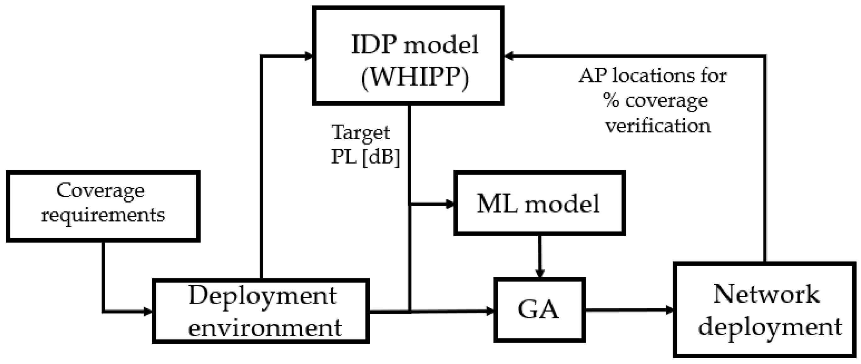
3.4.2. ML + GA Based Network Planning Approach

To find the deployment with a minimal number of 5G APs, while still providing the required quality of service, we used the architecture in Figure 1, and the link budget parameters from

Table 2. Parameter settings for the network optimization. CQI is the Channel Quality Indicator. SNR is the Signal to Noise Ratio. Rx is the minimal received power to satisfy the SNR requirement accounting for the given shadowing and fading margins.

Frequency	3500 MHz
Bandwidth	80 MHz
EIRP	20 dBm
Shadowing margin	7 dB
Fading Margin	5 dB
Thermal noise power at 300 K (@80 MHz bandwidth)	−95 dBm
CQI/Modulation/SNR/Bitrate/Rx [44]	CQI	Modulation	SNR [dB]	Bitrate [Mbps]	Rx [dBm]
	2	QPSK	−3	70	−86
	3	QPSK	0	96	−83
	4	16QAM	3	100	−80
	5	16QAM	5	188	−78
	12	256QAM	27	664	−56
	13	256QAM	29	774	−54
	15	256QAM	30	1000	−53

. The core of the architecture is a GA [13] taking as inputs the floor plan and the PL estimation (only one time calculation) made with the ML algorithm for every possible AP-Rx link (we refer the reader to Section 4.2.1 for more details). The output is a wireless network deployment with a minimal set of APs, that provides the required coverage at all the points inside the building, according to the ML-based PL model. It is then required to verify this coverage percentage with the actual IDP PL model.

Genetic Algorithm

Figure 2 shows a flow graph of the GA developed to find the minimal number of APs that can provide the required bit rate, according to the parameters from Table 2. Logically, Rx locations are excluded as possible AP locations in the optimization process. Each “individual” in the population corresponds to a possible network solution and is characterized by an array containing the state of the respective APs, where each AP corresponds to a gene of a solution. Every individual solution X_i, i = 1 …. population_size is represented by an M-dimensional vector, where M represents the number of candidate APs, of which the locations are set on a 4 m grid spanning the entire building (we refer the reader to Section 4.2 for more details). The parameter population_size is set to 100.

$$X_i=(X_{i,1}, X_{i,2},\dots .X_{i,M})$$

(5)

with $X_{i,j}$, j = 1 …. M, a gene of solution $X_i$, representing either switched off (set to 0) or switched on (set to 1).

The GA starts with an “Initialization” step during which the scenario parameters are set. It defines the Rx_Min, which is equal to the Rx threshold defined in Table 2 for each throughput. After the initialization phase, all candidate APs are randomly switched on (set to 1) or off (set to 0). Each iteration it (it = 1,…, max_it, max_it = 100) consists of the following consecutive steps.

• Sorting—sort all previous individuals (solutions) by their score values. The score is based on the characteristics of the solution, where coverage of all grid points is a hard requirement, and where a minimal number of deployed APs is desired, with (optionally) a maximal AVE_Rx value. This leads to the following score formula:

$$Score=2\left(100-co{v}_{perct}\right)+A{P}_{dep}+0.05\left(R{x}_{Min}-AV{E}_{Rx}\right)$$

(6)

where $co{v}_{perct}$ is the percentage of grid points that are covered with the minimum Rx level, $A{P}_{dep}$ is the sum of the active gene (APs switched on) of solution X_i (see Equation (3)), $R{x}_{Min}$ is equal to the Rx threshold defined in Table 2 for each throughput, and $AV{E}_{Rx}$ is the received signal level average of 100% of grid points.

• Crossover—from the sorted population, a new population is created where the best_individuals (five individuals) from the previous population are transferred unchanged to the new population. The other new child solutions (population_size—best_individuals) are obtained from a crossover operation between two individuals, each chosen as the fittest individual out of a set of 5 random individuals from the population of the previous generation. Each child gene is inherited from either one of the corresponding parent genes, with equal probability. The newly created child solution is added to the new population.
• Mutation—all individuals in the obtained new population are mutated. If the mutation has a better score than the original individual, the original individual in the population is replaced by the mutated individual. The mutation operation is as follows:

  ○

  If all receiver locations are not covered (Rx < Rx_Min), one random inactive AP is switched on

  ○

  If all receiver locations are covered (Rx ≥ Rx_Min), one random active AP is switched off

4. Results and Discussion

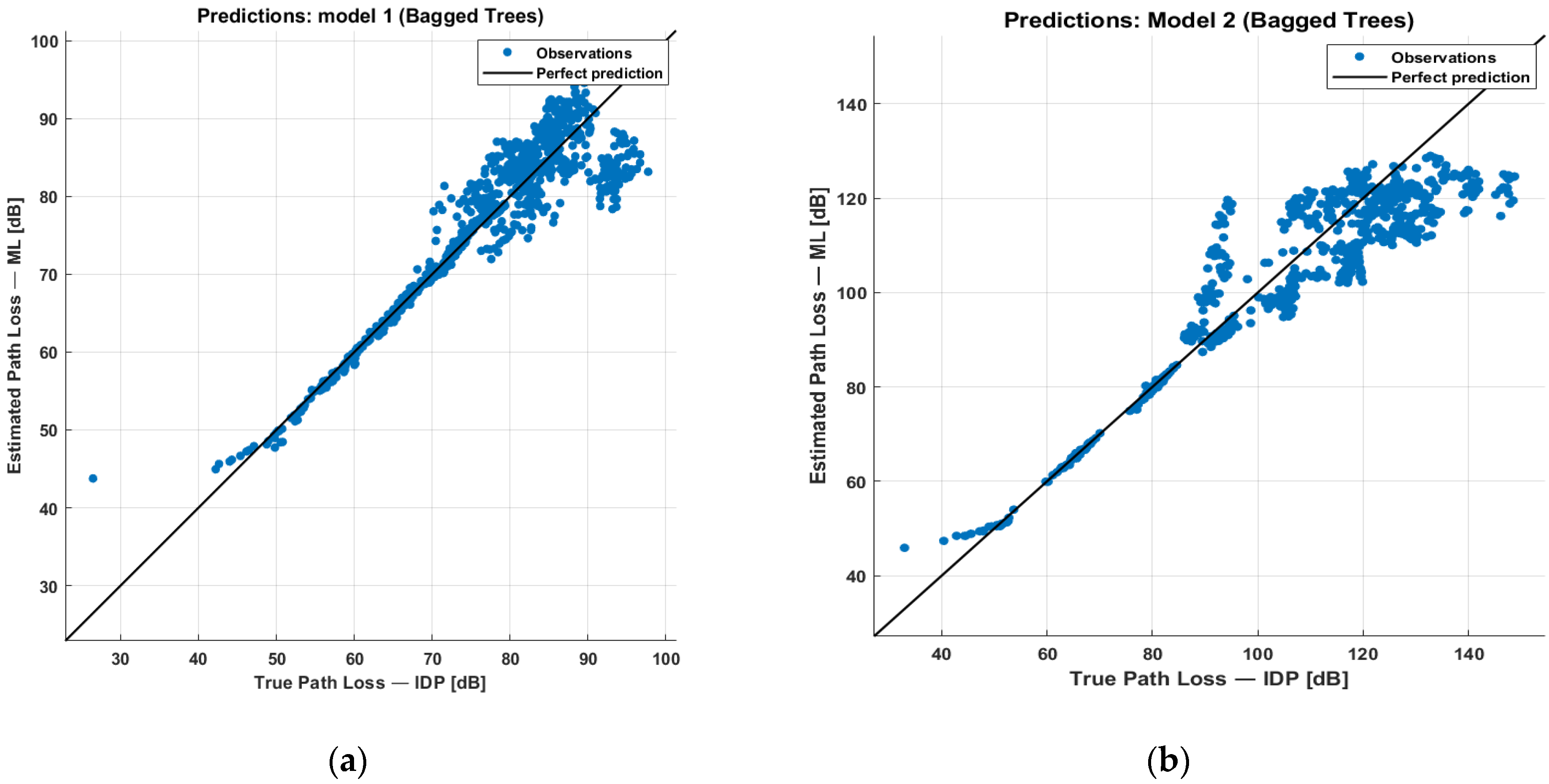
4.1. Machine Learning Model for PL Estimation

In Section 3.2 and Section 3.3, the resulting datasets for training/validating/testing the models were presented. Every one of them contains 11 parameters, 10 inputs, and 1 output resulting from the indoor environment and the physical locations of the AP and the receiver point. We analyzed two models based on the diffraction loss factor.

For model 1, we tested the constructed ML model using the iGent building and for model 2 using the Vooruit and Koutitas buildings. Figure 3 shows a scatter plot of the ML-estimated values vs. the assumed true values (WHIPP IDP estimation) for the two models. A perfect estimation would lie on the black line. It can be noticed that both models perform well, particularly for PL values from 50 dB up to around 80 dB. In network planning, the maximum allowable path loss determines if a receiver point is covered. So, the model will perform well, especially for low-power APs and high-throughput requirements, both of which impact the link budget and thus also the maximum allowable path loss.

To illustrate the accuracy of the path loss estimations, we compare the received power over the building area, as estimated by the proposed ML models and by the WHIPP IDP calculation (AP EIRP = 20 dBm). Figure 4 compares the simulated Rx due to a randomly placed AP, according to the WHIPP tool (1st row) and according to the ML PL model (2nd row) for the three buildings used in the testing process (samples not included in the training/validating dataset), i.e., iGent building for model 1, Vooruit and Koutitas buildings for model 2. The figure shows a good correspondence between both Rx calculations.

The absolute average difference between the WHIPP IDP model and the ML model is 2.5 dB for the iGent office building (Figure 4a), 2.3 dB for the Vooruit arts centre building (Figure 4(b.1)), and 1.3 dB for the Koutitas office building (Figure 4(b.2)).

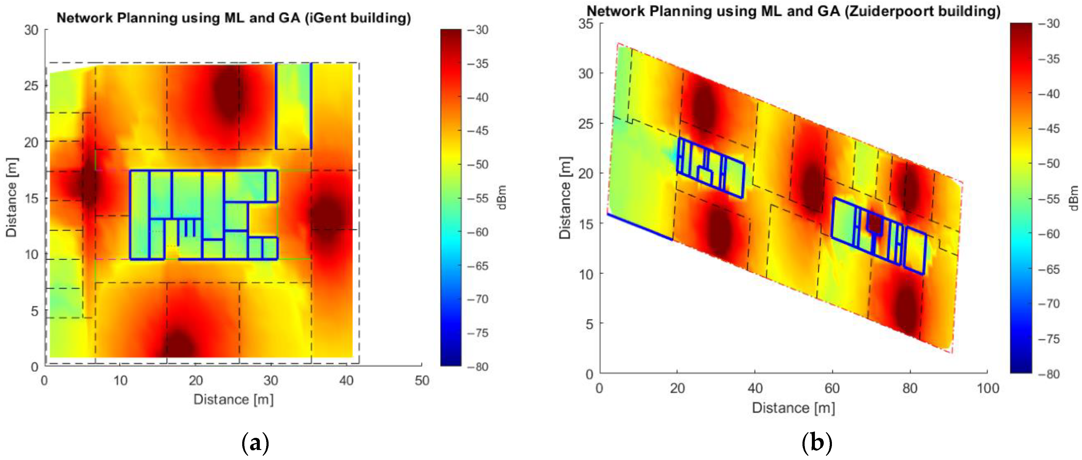
4.2. Network Planning Results and Performance

4.2.1. Wireless Network Planning for 664 Mbps

In a second phase, we can now use the quick and accurate ML model for network planning, using the GA as explained in Section 3.4. The reception quality specifications for the floors of the five buildings (Section 3.2) were taken from Table 2. Figure A1 (Appendix A) show the resulting network deployment for the floors of the five buildings. The deployments were designed based on the setting 12/256QAM/27dB/664 Mbps/-56dBm from Table 2, APs transmitting with an EIRP of 20 dBm, and without taking into consideration the maximum AVE_Rx for the whole floor.

Table 3. Comparison between the WHIPP and ML + GA network planners, with respect to the required number of APs, the time to calculate the network deployment, and the coverage percentage for the setting 12/256QAM/27dB/664 Mbps/-56dBm from Table 2.

Scenario	Possible APs	WHIPP Tool		ML + GA
		Required APs	Optimization Time [min]	Required APs	Pre-Processing Time [min]	GA Optimization Time [min]	% Rx Covered	AVERx Gain [dB]
iGent	52	4	7.15	4	83	0.11	99.37	3.80
Zuiderpoort	58	6	42.80	6	95	0.20	100.00	4.20
Vooruit	50	3	2.00	3	78	0.16	100.00	4.50
Koutitas	45	13	10.00	10	38	0.16	99.56	2.00
Library Jaume I	187	26	1358.00	26	480	1.56	100.00	3.00

compares the results from the WHIPP optimization with the one obtained using the proposed ML + GA approach. The coverage percentage of the GA-proposed deployment is evaluated by applying the WHIPP IDP PL model to the proposed ML-GA deployment. Both tools were built on the same set of candidate APs, obtaining a deployment with the same number of APs in almost all the cases. For the Koutitas building, however, only 10 APs were required (23% reduction) using the ML + GA approach, while 13 APs were required for the WHIPP tool. Hence, in terms of the required APs for network planning, our solution has similar, or better, performance than the WHIPP tool.

Table 3 confirms that the GA-proposed solution is reliable, as the coverage percentage with the aimed throughput is at least 99.37% (iGent building, 1105/1112 receiver points covered). In the Koutitas building, coverage was 99.56% (909/913) of the receiver points. The rest of the buildings have all grid points covered with the throughput that was aimed for. Furthermore, related to the time to make the planning, the GA optimization is much faster. It should be noted, though, that the ML PL calculation for all possible AP-Rx links requires a one-time calculation (Pre-processing Time in Table 3). However, these values can be re-used when another throughput requirement is set (see Section 4.2.3), when room-specific requirements are set, or when a maximal Rx is strived for (see Section 4.2.2), etc. The heuristic WHIPP algorithm, on the other hand, needs to re-execute the entire optimization algorithm for another throughput requirement and does not offer any flexibility that the GA can account for via its cost function.

4.2.2. Wireless Network Planning for 664 Mbps and a Maximal Average Received Power AVE_Rx

Table 4. Comparison between the WHIPP and ML + GA network planners, with respect to the required number of APs, the time to calculate the network deployment, and coverage percentage for the setting 15/256QAM/30 dB/1000 Mbps/-53 dBm from Table 2.

Scenario	Possible APs	WHIPP Tool		ML + GA
		Required APs	Time [min]	Required APs	GA Calculation Time [min]	% Rx Covered
iGent	52	7	1.82	7	0.14	100
Zuiderpoort	58	9	27.22	9	0.22	100
Vooruit	50	4	1.05	4	0.08	100
Koutitas	45	16	18.13	12	0.13	100
Library Jaume I	187	35	1709.00	31	2.58	100

(AVE_Rx gain [dB]) shows the results of the network deployment after targeting a maximal average received power over all grid points (AVE_Rx), maximizing the QoS. Figure A2 shows the resulting network deployment with the same setting as the deployment of Section 4.2.1, but accounting for a maximum AVE_Rx. It can be noticed that the AP distribution changed. In addition, to validate the approach of introducing this constraint, we evaluated the average received power of the GA-proposed deployment, according to the WHIPP IDP PL model. The results show that the average received power after applying the maximum AVE_Rx criterion is increased by 2.0 to 4.5 dB (see last column of Table 4). This indicates that the GA-proposed solution is able to maximize and homogenize the received signal level.

4.2.3. Wireless Network Planning for 1000 Mbps and a Maximal Average Received Power AVE_Rx

Finally, to further showcase the advantages of the ML + GA-approach over the WHIPP tool, Table 4 shows the results of the network design for a higher throughput requirement, being reflected by higher required received power (see Table 2, 15/256QAM/30 dB/1000 Mbps/−53 dBm). Table 4 shows that in the final proposed deployment 100% of Rx points are covered with the required signal strength. In terms of the number of APs, the ML + GA can find a better solution: 4 APs (25%) fewer for the Koutitas building and 4 APs (11%) fewer for the Library Jaume I building. Related to the time to make the deployment, the GA re-uses the preprocessed PL values calculated in the previous deployment, resulting in a calculation time that is in the worst case still 15 times faster than in the case of the WHIPP tool.

Above scenarios show that the ML model was able to accurately estimate PL calculated by more complex models with an MAE lower than 3 dB compared to an IDP-based path loss model. The same principles could equally be applied to other complex models that are based on physical inputs. It was subsequently shown that a GA using this ML model can find a better network deployment (with a lower number of APs) without compromising coverage and taking into account additional constraints like the maximum AVE_Rx.

5. Conclusions

We proposed a novel indoor network planning approach based on the combination of machine learning and a genetic algorithm. We used the Decision Tree Ensembles (Bagging) algorithm to build a generic model able to estimate the PL. The model was trained/validated with easy-to-calculate information from a building (e.g., number of walls between the AP and the point, total wall loss along the direct ray) and validated in three other buildings, yielding an MAE lower than 3 dB, compared to an advanced dominant path loss model accounting for physical characteristics of the environment. Subsequently, this ML model was used in a GA to perform network planning for finding a deployment with a minimal number of AP, and still delivering the required throughput. The results were compared to a heuristic optimizer in terms of the number of required APs to provide coverage, the time to calculate this deployment, and the deployment accuracy. The proposed ML + GA-based solution achieves the same, or better, results in the number of required AP to satisfy different reception conditions, is 15 times faster, and provides full flexibility towards replanning, with only minor impact on model performance.

Future work will consist of a time optimization for the features (inputs) calculation process, where the PL for all possible AP-grid point links is calculated to be used in the GA. A modification to the cost function in the GA will be added to target minimal human exposure, and a higher SIR. Finally, this approach will be tested for accurate wireless network planning using ray-tracing path loss models.

References

1. Dangi, R.; Lalwani, P.; Choudhary, G.; You, I.; Pau, G. Study and Investigation on 5G Technology: A Systematic Review. Sensors 2021, 22, 26. [Google Scholar] [CrossRef] [PubMed]
2. Ali, U.; Caso, G.; De Nardis, L.; Kousias, K.; Rajiullah, M.; Alay, Ö.; Neri, M.; Brunstrom, A.; Di Benedetto, M.-G. Large-Scale Dataset for the Analysis of Outdoor-to-Indoor Propagation for 5G Mid-Band Operational Networks. Data 2022, 7, 34. [Google Scholar] [CrossRef]
3. Adegoke, E.I.; Edwards, R.M.; Whittow, W.G.; Bindel, A. Characterizing the Indoor Industrial Channel at 3.5GHz for 5G. In 2019 Wireless Days (WD); IEEE: Piscataway, NJ, USA, 2019; pp. 1–4. [Google Scholar] [CrossRef]
4. Attaran, M. The impact of 5G on the evolution of intelligent automation and industry digitization. J. Ambient Intell. Humaniz. Comput. 2021, 1, 3. [Google Scholar] [CrossRef] [PubMed]
5. El Boudani, B.; Kanaris, L.; Kokkinis, A.; Kyriacou, M.; Chrysoulas, C.; Stavrou, S.; Dagiuklas, T. Implementing Deep Learning Techniques in 5G IoT Networks for 3D Indoor Positioning: DELTA (DeEp Learning-Based Co-operaTive Architecture). Sensors 2020, 20, 5495. [Google Scholar] [CrossRef] [PubMed]
6. Sheikh, M.U.; Mela, L.; Saba, N.; Ruttik, K.; Jantti, R. Outdoor to Indoor Path Loss Measurement at 1.8GHz, 3.5GHz, 6.5GHz, and 26GHz Commercial Frequency Bands. In Proceedings of the 2021 24th International Symposium on Wireless Personal Multimedia Communications (WPMC), Okayama, Japan, 14–16 December 2021; pp. 1–5. [Google Scholar] [CrossRef]
7. Diago-Mosquera, M.E.; Aragón-Zavala, A.; Rodriguez, M. Testing a 5G Communication System: Kriging-Aided O2I Path Loss Modeling Based on 3.5 GHz Measurement Analysis. Sensors 2021, 21, 6716. [Google Scholar] [CrossRef] [PubMed]
8. Samad, A.; Diba, F.D.; Kim, Y.-J.; Choi, D.-Y. Results of Large-Scale Propagation Models in Campus Corridor at 3.7 and 28 GHz. Sensors 2021, 21, 7747. [Google Scholar] [CrossRef]
9. Ullah, U.; Kamboh, U.R.; Hossain, F.; Danish, M. Outdoor-to-Indoor and Indoor-to-Indoor Propagation Path Loss Modeling Using Smart 3D Ray Tracing Algorithm at 28 GHz mmWave. Arab. J. Sci. Eng. 2020, 45, 10223–10232. [Google Scholar] [CrossRef]
10. Teh, C.H.; Chung, B.K.; Lim, E.H. Multilayer Wall Correction Factors for Indoor Ray-Tracing Radio Propagation Modeling. IEEE Trans. Antennas Propag. 2019, 68, 604–608. [Google Scholar] [CrossRef]
11. Fathurrahman, S.Z.; Rahardjo, E.T. Coverage of Radio Wave Propagation at UI Campus Surrounding Using Ray Tracing and Physical Optics Near to Far Field Method. In Proceedings of the TENCON 2018—2018 IEEE Region 10 Conference, Jeju, Korea, 28–31 October 2018; pp. 1123–1126. [Google Scholar] [CrossRef]
12. Plets, D.; Joseph, W.; Vanhecke, K.; Tanghe, E.; Martens, L. Coverage prediction and optimization algorithms for indoor environments. EURASIP J. Wirel. Commun. Netw. 2012, 2012, 123. [Google Scholar] [CrossRef] [Green Version]
13. Zhu, W.; Huang, C.-L.; Yeh, W.-C.; Jiang, Y.; Tan, S.-Y. A Novel Bi-Tuning SSO Algorithm for Optimizing the Budget-Limited Sensing Coverage Problem in Wireless Sensor Networks. Appl. Sci. 2021, 11, 10197. [Google Scholar] [CrossRef]
14. Zhang, Y.; Wen, J.; Yang, G.; He, Z.; Wang, J. Path Loss Prediction Based on Machine Learning: Principle, Method, and Data Expansion. Appl. Sci. 2019, 9, 1908. [Google Scholar] [CrossRef] [Green Version]
15. Tognola, G.; Plets, D.; Chiaramello, E.; Gallucci, S.; Bonato, M.; Fiocchi, S.; Parazzini, M.; Martens, L.; Joseph, W.; Ravazzani, P. Use of Machine Learning for the Estimation of Down- and Up-Link Field Exposure in Multi-Source Indoor WiFi Scenarios. Bioelectromagnetics 2021, 42, 550–561. [Google Scholar] [CrossRef] [PubMed]
16. Trogh, J.; Plets, D.; Martens, L.; Joseph, W. Advanced Real-Time Indoor Tracking Based on the Viterbi Algorithm and Semantic Data. Int. J. Distrib. Sens. Networks 2015, 11, 271818. [Google Scholar] [CrossRef]
17. Cheng, H.; Lee, H.; Ma, S. CNN-Based Indoor Path Loss Modeling with Reconstruction of Input Images. In Proceedings of the 2018 International Conference on Information and Communication Technology Convergence (ICTC), Jeju, Korea, 17–19 October 2018; pp. 605–610. [Google Scholar] [CrossRef]
18. Diba, F.D.; Samad, A.; Choi, D.-Y. Centimeter and Millimeter-Wave Propagation Characteristics for Indoor Corridors: Results from Measurements and Models. IEEE Access 2021, 9, 158726–158737. [Google Scholar] [CrossRef]
19. Ma, S.; Cheng, H.; Lee, H. A Practical Approach to Indoor Path Loss Modeling Based on Deep Learning. J. Comput. Sci. Eng. 2021, 15, 84–95. [Google Scholar] [CrossRef]
20. Zhang, Y.; Wen, J.; Yang, G.; He, Z.; Luo, X. Air-to-Air Path Loss Prediction Based on Machine Learning Methods in Urban Environments. Wirel. Commun. Mob. Comput. 2018, 2018, 8489326. [Google Scholar] [CrossRef]
21. Goudos, S.K.; Athanasiadou, G.; Tsoulos, G.V.; Rekkas, V. Modelling Ray Tracing Propagation Data Using Different Machine Learning Algorithms. In Proceedings of the 2020 14th European Conference on Antennas and Propagation (EuCAP), Copenhagen, Denmark, 15–20 March 2020. [Google Scholar] [CrossRef]
22. Apavatjrut, A.; Kamdee, S. On Optimizing WiFi RSSI and Channel Assignment using Genetic Algorithm for WiFi Tuning. ECTI Trans. Electr. Eng. Electron. Commun. 2021, 19, 322–330. [Google Scholar] [CrossRef]
23. Liu, N.; Plets, D.; Joseph, W.; Martens, L. An algorithm for optimal network planning and frequency channel assignment in indoor WLANs. In Proceedings of the 2014 IEEE Antennas and Propagation Society International Symposium (APSURSI), Memphis, TN, USA, 6–11 July 2014; pp. 1177–1178. [Google Scholar] [CrossRef] [Green Version]
24. Qiu, S.; Chu, X.; Leung, Y.-W.; Ng, J.K.Y. Joint Access Point Placement and Power-Channel-Resource-Unit Assignment for 802.11ax-Based Dense WiFi with QoS Requirements. In Proceedings of the IEEE INFOCOM 2020—IEEE Conference on Computer Communications, oronto, ON, Canada, 6–9 July 2020; pp. 2569–2578. [Google Scholar] [CrossRef]
25. Vilovic, I.; Burum, N.; Sipus, Z. Design of an indoor wireless network with neural prediction model. In Proceedings of the Second European Conference on Antennas and Propagation, EuCAP 2007, Edinburgh, UK, 11–16 November 2007. [Google Scholar] [CrossRef]
26. Zhang, Z.; Di, X.; Tian, J.; Zhu, Z. A multi-objective WLAN planning method. In Proceedings of the 2017 International Conference on Information Networking (ICOIN), Da Nang, Vietnam, 11–13 January 2017; pp. 86–91. [Google Scholar] [CrossRef]
27. Abdallah, W.; Mnasri, S.; Val, T. Distributed Approach for the Indoor Deployment of Wireless Connected Objects by the Hybridization of the Voronoi Diagram and the Genetic Algorithm. arXiv 2022, arXiv:2202.13735. [Google Scholar] [CrossRef]
28. Lee, B.-H.; Ham, D.; Choi, J.; Kim, S.-C.; Kim, Y.-H. Genetic Algorithm for Path Loss Model Selection in Signal Strength-Based Indoor Localization. IEEE Sens. J. 2021, 21, 24285–24296. [Google Scholar] [CrossRef]
29. Mohammed, R.A.; Salim, O.N.M.; Al-Nakkash, A.H.; AlAbdullah, A.A.S. Proposed APs Distribution Optimization Algorithm: Aware of Interference (APD-AI). IOP Conf. Ser. Mater. Sci. Eng. 2020, 745, 12040. [Google Scholar] [CrossRef]
30. Zhang, J.; Li, J.; Cai, M.; Li, D.; Wang, Q. The 5G NOMA networks planning based on the multi-objective evolutionary algorithm. In Proceedings of the 2020 16th International Conference on Computational Intelligence and Security (CIS), Guangxi, China, 27–30 November 2020; pp. 59–62. [Google Scholar] [CrossRef]
31. Omae, M.O.; Ndungu, E.N.; Kibet, P.L. Indoor LOS Wi-Fi Signal Coverage Modeling Using PSO Trained LOG10D-ANFIS with Random Input. Int. J. Sci. Eng. Res. 2019, 10, 1151–1158. [Google Scholar]
32. Abdallah, W.; Val, T. Genetic-Voronoi algorithm for coverage of IoT data collection networks. 30th International Conference on Computer Theory and Applications (ICCTA 2020), Alexandria, Egypt, 12–14 December 2020. [Google Scholar] [CrossRef]
33. Wölfle, G.; Wahl, R.; Wertz, P.; Wildbolz, P.; Landstorfer, F. Dominant Path Prediction Model for Indoor Scenarios. In German Microwave Conference (GeMIC); University of Ulm: Ulm, Germany, 2005; Volume 27. [Google Scholar]
34. Wolfle, G.; Landstorfer, F.M.; Gahleitner, R.; Bonek, E. Extensions to the field strength prediction technique based on dominant paths between transmitter and receiver in indoor wireless communications. In Proceedings of the 2nd European Personal and Mobile Communications Conference (EPMCC), Bonn, Germany, 30 September–2 October 1997. [Google Scholar]
35. Keenan, J.M.; Motley, A.J. Radio coverage in buildings. Br. Telecom Technol. 1990, 8, 19–24. [Google Scholar]
36. Breiman, L. Bagging predictors. Mach. Learn. 1996, 24, 123–140. [Google Scholar] [CrossRef] [Green Version]
37. Lomte, S.S.; Torambekar, S.G. Decision Tree for Uncertain Numerical Data Using Bagging and Boosting; Nagar, A.K., Jat, D.S., Marín-Raventós, G., Mishra, D.K., Eds.; Springer Singapore: Singapore, 2022; pp. 509–523. [Google Scholar]
38. Yadav, S.; Shukla, S. Analysis of k-fold cross-validation over hold-out validation on colossal datasets for quality classification. In Proceedings of the 2016 IEEE 6th International Conference on Advanced Computing (IACC), Bhimavaram, India, 27–28 February 2016; pp. 78–83. [Google Scholar]
39. Efron, B. Bootstrap Methods: Another Look at the Jackknife. Ann. Stat. 1979, 7, 1–26. [Google Scholar] [CrossRef]
40. Ensemble Methods: Bagging, Boosting and Stacking|By Joseph Rocca|Towards Data Science. Available online: https://towardsdatascience.com/ensemble-methods-bagging-boosting-and-stacking-c9214a10a205 (accessed on 1 April 2022).
41. Koutitas, G.; Samaras, T. Exposure Minimization in Indoor Wireless Networks. IEEE Antennas Wirel. Propag. Lett. 2010, 9, 199–202. [Google Scholar] [CrossRef]
42. Mahmood, T.; Al-Qaysi, H.K.; Hameed, A.S. The Effect of Antenna Height on the Performance of the Okumura/Hata Model under Different Environments Propagation. In Proceedings of the 2021 International Conference on Intelligent Technologies (CONIT), Hubli, India, 25–27 June 2021; pp. 1–4. [Google Scholar] [CrossRef]
43. Akhpashev, R.V.; Andreev, A.V. COST 231 Hata adaptation model for urban conditions in LTE networks. In Proceedings of the 2016 17th International Conference of Young Specialists on Micro/Nanotechnologies and Electron Devices (EDM), Erlagol, Russia, 30 June–4 July 2016; pp. 64–66. [Google Scholar] [CrossRef]
44. Chu, E.; Yoon, J.; Jung, B.C. A Novel Link-to-System Mapping Technique Based on Machine Learning for 5G/IoT Wireless Networks. Sensors 2019, 19, 1196. [Google Scholar] [CrossRef] [Green Version]
Figure 1. Flow graph of the network optimization algorithm and its validation with the WHIPP tool.
Applsci 12 03923 g001
Figure 2. Flow graph of Genetic Algorithm for network deployment.
Applsci 12 03923 g002
Figure 3. Comparison between the IDP path loss values and the ML-estimated ones for (a) Model 1 and (b) Model 2.
Applsci 12 03923 g003
Figure 4. Received power according to WHIPP IDP model (1st row) versus the estimation using the ML models (2nd row) with an R2 = 0.94. Received power (a) using PL Model 1 and testing on the iGent building. (b) using PL Model 2 and testing on Vooruit (b.1), and Koutitas (b.2) buildings.
Applsci 12 03923 g004