
Delay Analysis and the Control of Electro-Hydrostatic Actuators


1
College of Energy and Power Engineering, Nanjing University of Aeronautics and Astronautics, Nanjing 210016, China
2
Nanjing Research Institute, Huawei Technologies Co., Ltd., Nanjing 210012, China
*
Author to whom correspondence should be addressed.
Appl. Sci. 2022, 12(6), 3089; https://doi.org/10.3390/app12063089
Submission received: 30 January 2022
/
Revised: 9 March 2022
/
Accepted: 15 March 2022
/
Published: 17 March 2022
Abstract
:The electro-hydrostatic actuator (EHA) has a high energy density and a compact structure so it is widely used in all/more electric aircraft. To gain energy-saving capability, the hydraulic lock can be applied in the EHA system, which can overcome the change of load after the position control is complete, reducing the motor’s need to work continuously. Due to the use of a hydraulic lock in the EHA system, there is a more significant position output delay compared with the EHA system. The delay would lead to a dynamic response error. Therefore, an electro-hydrostatic actuator with a bidirectional hydraulic lock (BHL-EHA) model is established that can reflect the position output delay and it can be used to analyze its influence factors. According to the analysis, the factors affecting the delay are pump speed, external load, hydraulic lock cracking pressure, friction load, pump displacement, fluid volume of the system, and effective bulk modulus; thus, an equation that can be used to calculate the delay is proposed. At the same time, the experimental system of the BHL-EHA system is established, and the parameters of the experimental facility are completely consistent with the simulation model. Finally, a delay compensation control method is proposed, and the control time parameter is calculated based on the equation proposed above. The results of the simulation and the experiment show that the method can compensate for the delay caused by the hydraulic lock. Combined with a feedforward control, the method can dismiss the dynamic response error of 0.6 Hz sinusoidal tracking characteristics.
1. Introduction
In aviation, more electric aircraft (MEA) is becoming a hotspot as it outperforms traditional aircraft in terms of weight reduction, performance improvement, and increasing efficiency [1,2]. The “more electric” that uses electricity as the primary power source for the control system can reduce the number of power transfer systems. It utilizes the potential of ultra-reliable miniaturized power electronics, fault-tolerant electrical distribution systems, and electric generator/motor drives/actuators to increase performance and to reduce costs [3,4]. A power-by-wire (PBW) flight control system is the critical technology for MEA. It removes the centralized hydraulic system to obtain the advantages of the MEA, promoting broad use of electro-hydrostatic actuators (EHA). The EHA system is a form of PBW and the PBW makes the system more reliable. The PBW increases efficiency of MEA, and is needed in next generation all-electric aircraft (AEA) [5]. It is widely recognized that the EHA is an essential component of PBW [6,7,8].
Electro-hydrostatic actuators (EHA) were proposed in the 1990s, allowing the transmission of power from the electric to the hydraulic [9,10,11]. Compared to the traditional electro-hydraulic control system, the EHA system uses PBW technology that has high energy density, making it stand out from the numerous actuator systems and become a research hotspot for aircraft control [12,13]. In 1992, Joel R S applied EHA in the F-18 control system, and an experimental verification was performed on the flaps of the F18 in 1994 [14], which obtained an excellent result. Over the past decades, EHA has been applied to aircraft successfully.
Due to the incompressibility of oil, the hydraulic lock can keep the position output of the EHA system unchanged when the load changes. To further save energy and to avoid the energy loss caused by the continuous operation of the motor when the load changes or the pump becomes a hydraulic motor due to the load change after the motor stops working, the hydraulic lock is applied in the EHA system to realize an internal contracting brake. As mentioned above, the EHA is applied to the MEA, and the EHA system can be used in the control of the MEA on the angle of the compressor guide vane. The angle of the compressor guide vane is adjusted only when the rotor speed changes greatly, but the load of the aeroengine guide vane on the EHA system is constantly changing. Therefore, the position control of the aeroengine guide vane angle needs a low response speed, so the BHL-EHA system has good adaptability, which makes full use of the advantages brought by the hydraulic lock that is applied in the EHA system.
However, the EHA has a position delay output, especially when the load is large or the hydraulic lock is applied in the system. Particularly when the motor speed of the EHA system is low, the delay is especially obvious. So, it is still necessary to analyze the delay of the BHL-EHA system with a low-rated motor speed.
The reason for the delay is that it takes time for the pressure to reach the threshold that can start the piston cylinder in the EHA system. So, the factor that influences the pressure and the pressure requirement needs to be analyzed.
Nawaz proposed the EHA with a pressure accumulator [15] to maximize efficiency, but they did not use hydraulic locks and the delay in their system is not significant. Kang Rongjie proposed an EHA system with two pressure accumulators and an electromagnetic valve as a hydraulic lock [16]. Although the pressure accumulator improves the dynamic performance of the EHA, it gains the weight of the EHA and they did not study the delay. Many EHA systems realize the hydraulic lock using an electromagnetic valve [16,17], which can reduce the delay by controlling the electromagnetic valve, but it makes control more complicated. References [18,19] introduced the pilot check valve as the hydraulic lock, but the influence of the hydraulic lock was not studied, and the delay was not shown in their study. Altare proposed a novel structure of the EHA [20] in which the hydraulic lock and the pressure accumulator were applied, and it obtained a good control effect. However, the pressure accumulator increased the weight of the EHA, and the hydraulic locks they used had a more complex structure. Beyond that, the effect of the hydraulic lock was not studied in their paper, so it is unknown whether the hydraulic lock they used would influence the delay. In 2010, Triet Hung Ho proposed a new hydraulic closed-loop hydrostatic transmission energy-saving system. The hydraulic lock consisted of check valves that could prevent flowing back and the cavitation problem [21]. However, using the hydraulic lock ensures the system works typically to save energy, which is different from the EHA system. As the system Triet proposed was not an EHA system, the delay was not the focus of their research. Hoai An Trinh proposed a fault estimation and fault-tolerant control strategy with two observers for a pump-controlled electro-hydraulic system (PCEHS) [22]. The system had the same structure as the EHA studied in our paper, which also uses a hydraulic lock composed of a check valve. In Hoai’s study, their control method achieved excellent control results, but they did not consider the impact of delay.
Lasse Schmidt researched improving the efficiency and the dynamic properties in a system control in which a hydraulic lock was used to ensure self-locking [23]. In their study, a delay occurred. They designed a control methodology to minimize it. The study of the delay in their paper could help us to analyze the delay caused by the hydraulic lock, but they did not analyze the influence factor of the delay. Daniel Hagen investigated a self-contained electro-hydraulic cylinder (SSC) in which the hydraulic lock consisted of two pilot-operated check valves. In their SSC, they used the hydraulic lock to take care of passive load-holding [24]. However, it was selected by the electrically operated on/off valves (EV), which was different from the hydraulic lock that influenced the delay. Damiano Padovani researched the SSC with passive load-holding capability in which the arrangement of the hydraulic lock consisting of pilot-operated check valves was debated [25]. Their study shed some light on the research of the system’s stability using hydraulic locks, and it should be appreciated. Søren Ketelsen used an indirectly controlled hydraulic lock consisting of two valves that were closed unless the pilot pressure was high enough to open the valve against the spring force [26]. The hydraulic lock they used would not affect the controls, and in their study the delay was ignored. Many other authors have tried to optimize the performance of the traditional EHA system using control methods. Reference [27] used quantitative feedback theory to optimize the steady-state and transient position tracking performances, but the EHA they used in their study did not show a delay. In [28], a combination with a feedback modulator, self-resonance cancellation, and a self-resonance cancellation disturbance observer was used and it drastically improved the control performance. They conducted the methods on a traditional EHA system, so they did not use the hydraulic lock and the delay was not obvious in their study.
Based on the structure proposed by Sweeney [18], we built a model of BHL-EHA to display the phenomenon of position output delay. There are different models of the EHA [29,30,31]. Some of them describe the behavior of components to analyze the dynamics of the EHA. However, the model they built does not show the delay. There are many software packages for modeling hydraulic systems. For example, Ning established the hydraulic model of a piston pump in AMESIM [32]. The AMESIM software is a multi-disciplinary modeling and simulation platform for complex systems with many hydraulic components. In the AMESIM library, the available model showing the poppet position of the piloted check valve can be found. So, AMESIM is considered an excellent software to build the model.
This paper modeled the BHL-EHA based on the component characteristics using a method combining MATLAB and AMESIM. The delay in the BHL-EHA system is fully analyzed and a delay compensation control method is proposed based on the analysis. According to the analysis, the factors affecting the delay are pump speed, external load, hydraulic lock cracking pressure, friction load, pump displacement, the fluid volume of the system, and effective bulk modulus; thus, an equation that can be used to calculate the delay is proposed. Based on the model, an experimental facility was built to prove the correctness of the model and to verify the control method. Section 2 details the modeling of the BHL-EHA and the experimental facility that was built based on the model. In Section 3, a stability analysis of the system with the delay is conducted and the position output delay is analyzed based on the model proposed in Section 2, and the experimental verification is carried out. Section 4 proposes a delay compensation control method and the results of the simulation and the experiment are analyzed and displayed. Finally, in Section 5, the results and the discussion highlight the advantages of this paper.
2. Materials and Methods
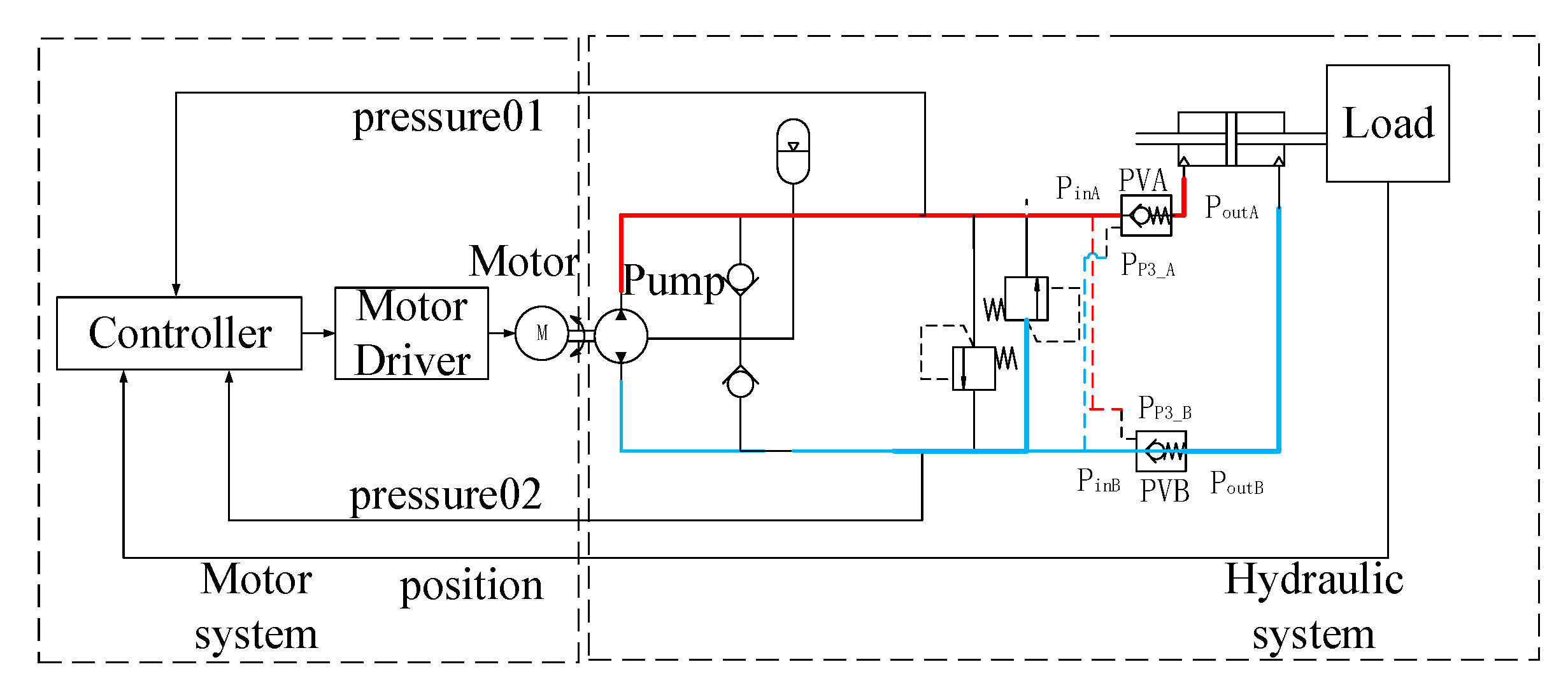
Figure 1 shows the BHL-EHA system structure. The EHA system consists of a motor, bidirectional gear pump, piston cylinder, fuel tank, check valve, an overflow valve, an electronic controller, a hydraulic lock, and an auxiliary component [18]. The position control of the piston-cylinder is realized by adjusting the motor’s speed and direction. The pump provides pressure and flows to the hydraulic system. The hydraulic lock is located at the front of the piston-cylinder in the hydraulic system. The position of the piston-cylinder is locked when there is no flow through the hydraulic lock.
As shown in Figure 1, the EHA system can be divided into the motor and the hydraulic systems. The output torque and the speed of the motor system are equal to the input torque and the speed of the hydraulic system. The motor system can be easily modeled in MATLAB using SIMULINK, and the hydraulic system can be conveniently modeled in AMESIM [33]. The interface of the two simulation platforms makes it possible to co-simulate in AMESIM and SIMULINK [34]. Therefore, the hydraulic system model is established in AMESIM, and the motor system model is established in SIMULINK.
Based on the model of the EHA system, the experimental facility can be built and the structure of the experimental facility is the same as the model. The parameters of the model are set according to the parameters of the experimental facility, so the simulation result of the model is in good agreement with the experiment’s result for the experimental facility.
2.1. Model of the Motor System
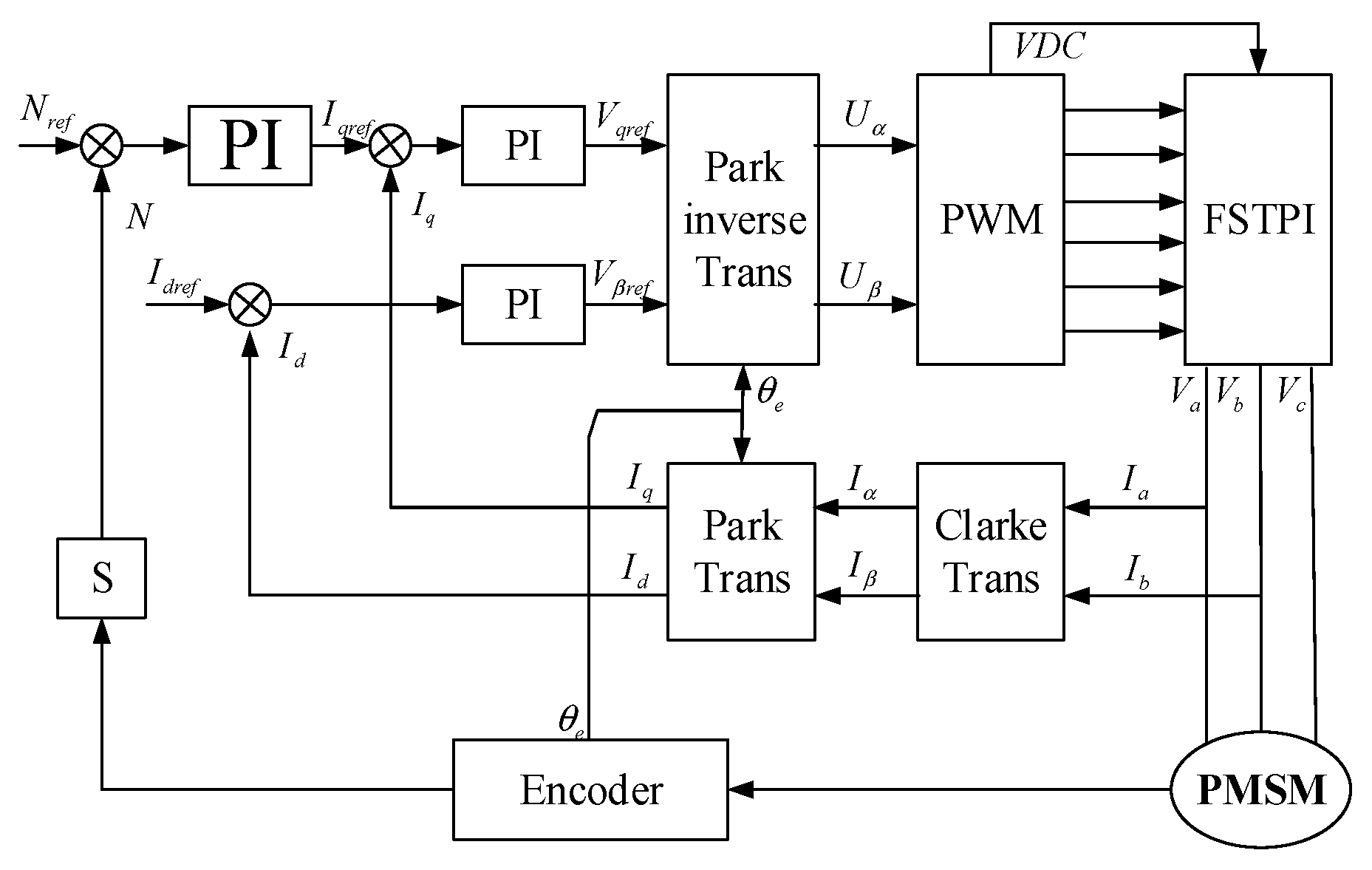
Due to the nonlinear factors of the motor, the linear model in the form of the transfer function is not sufficient to accurately describe the characteristics of the system. Thus, we use the MATLAB/SIMULINK interface that provides various nonlinear functions for modeling. The MATLAB model of the permanent magnet synchronous motor (PMSM) is established. Figure 2 shows the structure diagram of the PMSM system.
As shown in Figure 2, the voltage and the current of the PMSM can be transformed from the ABC coordinates to the d-q coordinates by using the Clarke transformation and the Park transformation. The encoder obtains the rotor position for transformation calculation. The double PI controller is used to adjust the rotational speed. A PI speed controller is adopted in the speed loop, and a vector controller is used in the current loop. In the current loop, the Id = 0 method is used [35]. The voltage in the d-q coordinates can be transformed to coordinates through the Park inverse transformation, generating the control signal to control the SVPWM controller. The SVPWM controller generates the SVPWM signal by using a three-phase inverter (FSTPI). In the d-q coordinates, the relationships of the motor voltage, current, and speed are as follows [34]:
where , , , is the voltage (V) and the current (A) of the motor under q-axis and d-axis, respectively. The inductance of the q-axis and the d-axis are and . The electromagnetic angular velocity is .
The [35], and the electromagnetic torque is:
and the angular velocity is:
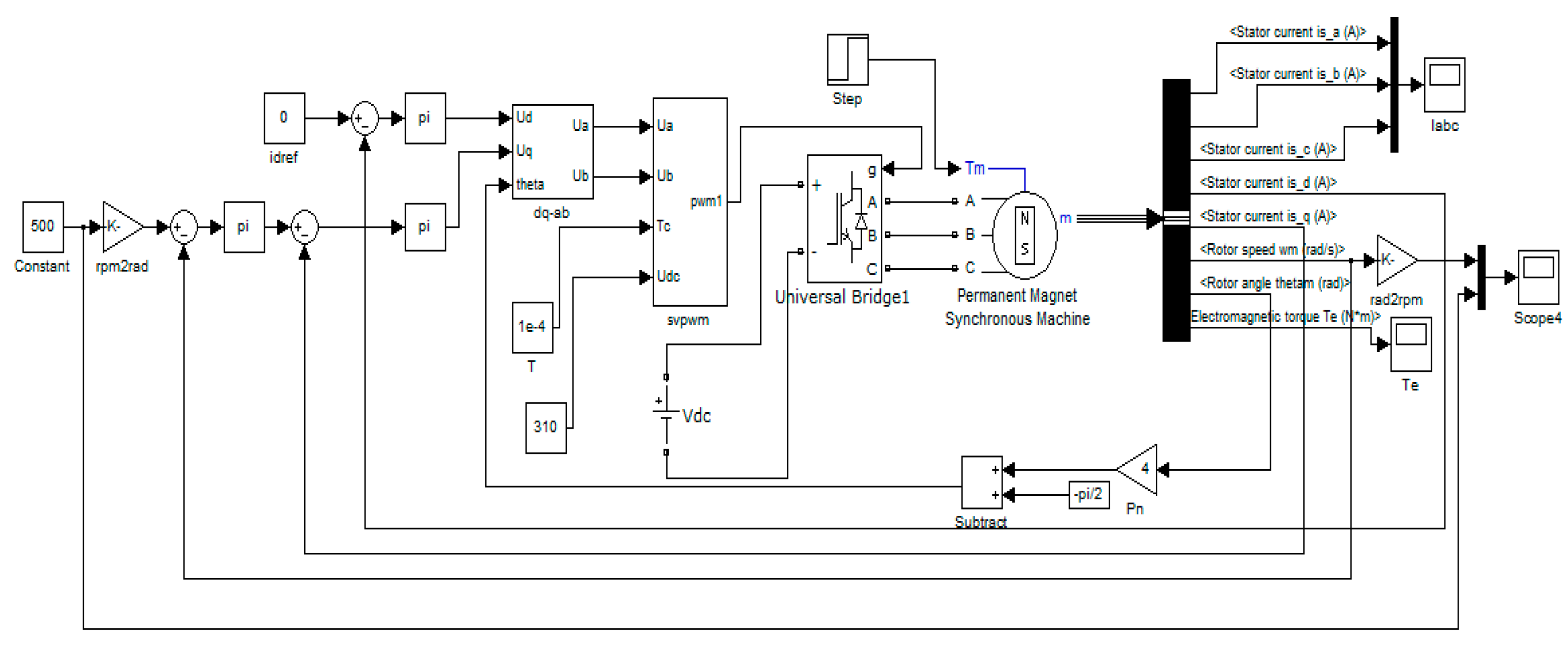
according to Equations (1)–(5), the model of PMSM is as shown in Figure 3. A PMSM component in SIMULINK is used. The Universal Bridge1 is the FSTPI. The Tm in Figure 3 is the torque of the pump, and the constant 500 in the figure is the rotational speed that is used to test the model.
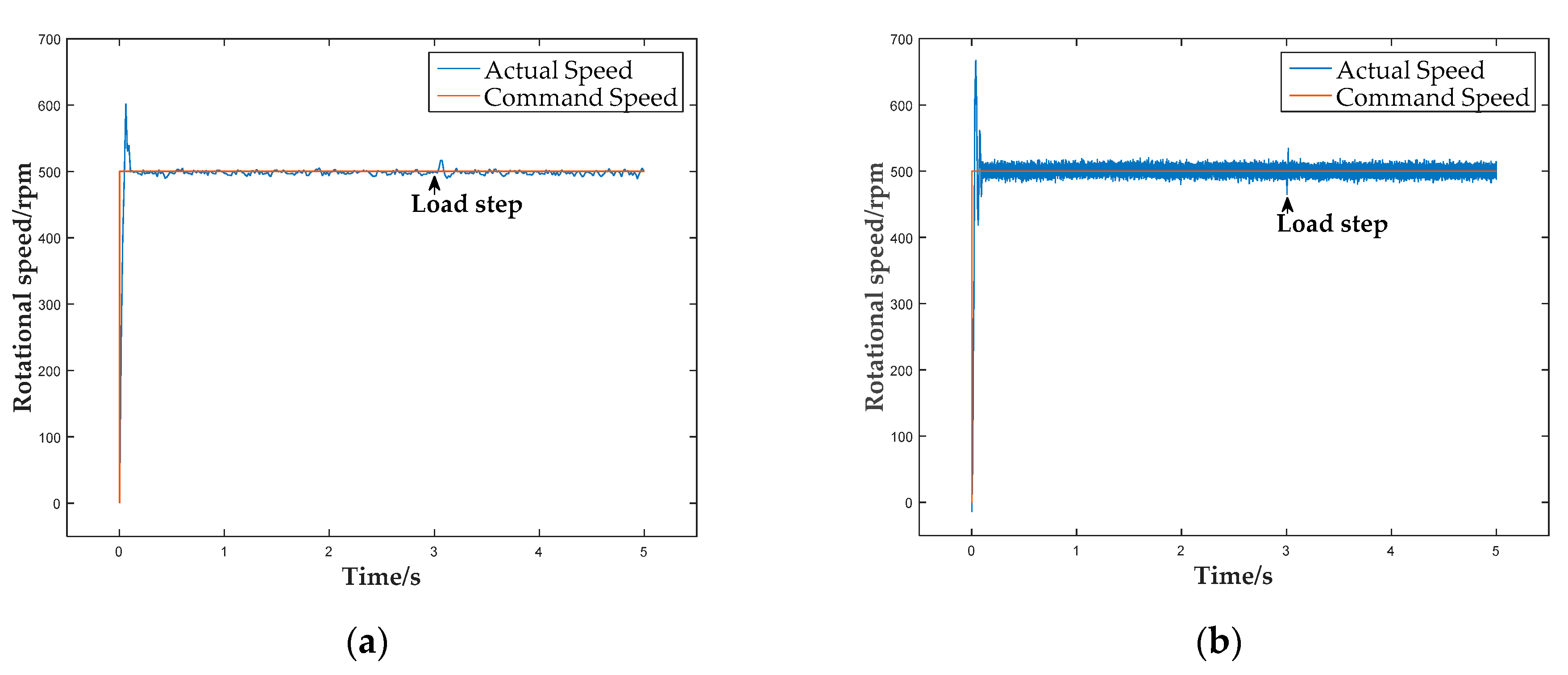
The PMSM’s parameters is shown in Table 1. The parameters of the PMSM are set according to the PMSM that will be used in the experimental facility. The rated speed affects the working limit of the motor. Since the delay of the BHL-EHA system is particularly obvious at low motor speed, the maximum speed of the motor is limited to 500 RPM to fully display this phenomenon. Figure 4 shows the result of the motor’s simulation and the experiment.
As shown in Figure 4, in the experiment, the overshoot is approximately 150 RPM, while in the simulation it is approximately 100 RPM. The setting time is approximately 0.10 s in the experiment, while in the simulation it is 0.08 s. It indicates that the simulation can reflect the experimental facility’s characteristics, and the control method of the experiment can achieve a good result.
2.2. Model of Hydraulic System
The most basic EHA hydraulic system consists of a hydraulic pump and a piston-cylinder. There are also many nonlinear factors in the hydraulic system. Therefore, the AMESIM was used to build a hydraulic system model, which could better reflect the characteristics of the hydraulic components. As the hydraulic system’s power element, the hydraulic pump can convert the mechanical energy into hydraulic energy and transfer energy to the piston cylinder to push the load. The flow of the pump can be calculated as follows:
is the input speed of the hydraulic pump, , is the inner leakage constant and outer leakage constant, and are the outlet and the inlet pressure of the pump. The motor drives the hydraulic pump, and the pump’s input torque is equal to the motor’s output torque. The output torque of the pump is:
where the torque of the friction and the moment of inertia of the pump are ignored. The friction and the moment of inertia can be ignored when the load is large enough.
The bidirectional hydraulic lock is a kind of pressure protection element composed of two parallel piloted check valves, and they cross-connect the inlet and the pilot port. The hydraulic lock can overcome the influence caused by the load’s disturbance, but it may lead to a delay. Therefore, the hydraulic lock is a critical component that should be analyzed.
The mechanical structure and the symbol of the hydraulic lock are shown in Figure 5. The piloted check valve A is located at the inlet of the piston-cylinder, while the piloted check valve B is located at the outlet.
The opening of the valve satisfies the function [34].
The dimensionless valve opening is , and are the inlet and the outlet pressure of the valve, is the check valve cracking pressure, is the pilot pressure, ratio is the pilot area ratio, and is the equivalent spring rate.
When the valve is not fully opened, it is equivalent to a throttle. The flow is associated with differential pressure and dimensionless valve opening [34]:
The flow coefficient is k, is the pressure difference of the inlet and the outlet of the valve, and is the fluid density.
The valve is fully open when the pilot pressure reaches the following condition [34].
According to Equations (8)–(10), the expression of the check valve is:
According to the above Equation (9), the hydraulic lock may cause a delay. When the valve is not open, the output of flow is 0. When the valve is open, the flow starts to output. The delay time depends on the valve opening time.
The piston cylinder is the primary execution component of the hydraulic system, which outputs force and displacement, according to the flow rate continuity and the force balance equation:
Then, the mathematical model of the piston cylinder can be obtained. Where is the total leakage coefficient of the piston cylinder, is the bulk modulus of elasticity of the oil, is the working chamber volume of the piston cylinder, is the output force, is the total mass of the load, is the viscous damping coefficient, and is the stiffness coefficient of the load.
Figure 6 shows the open-loop model in AMESIM. The hydraulic lock in Figure 6 is built according to the structure of the hydraulic lock in Figure 5 to reflect the characteristics of the hydraulic lock.
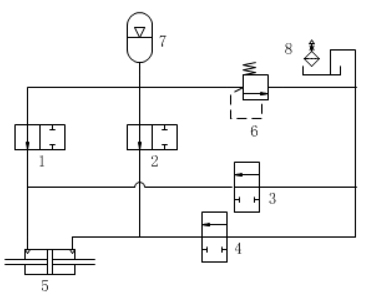
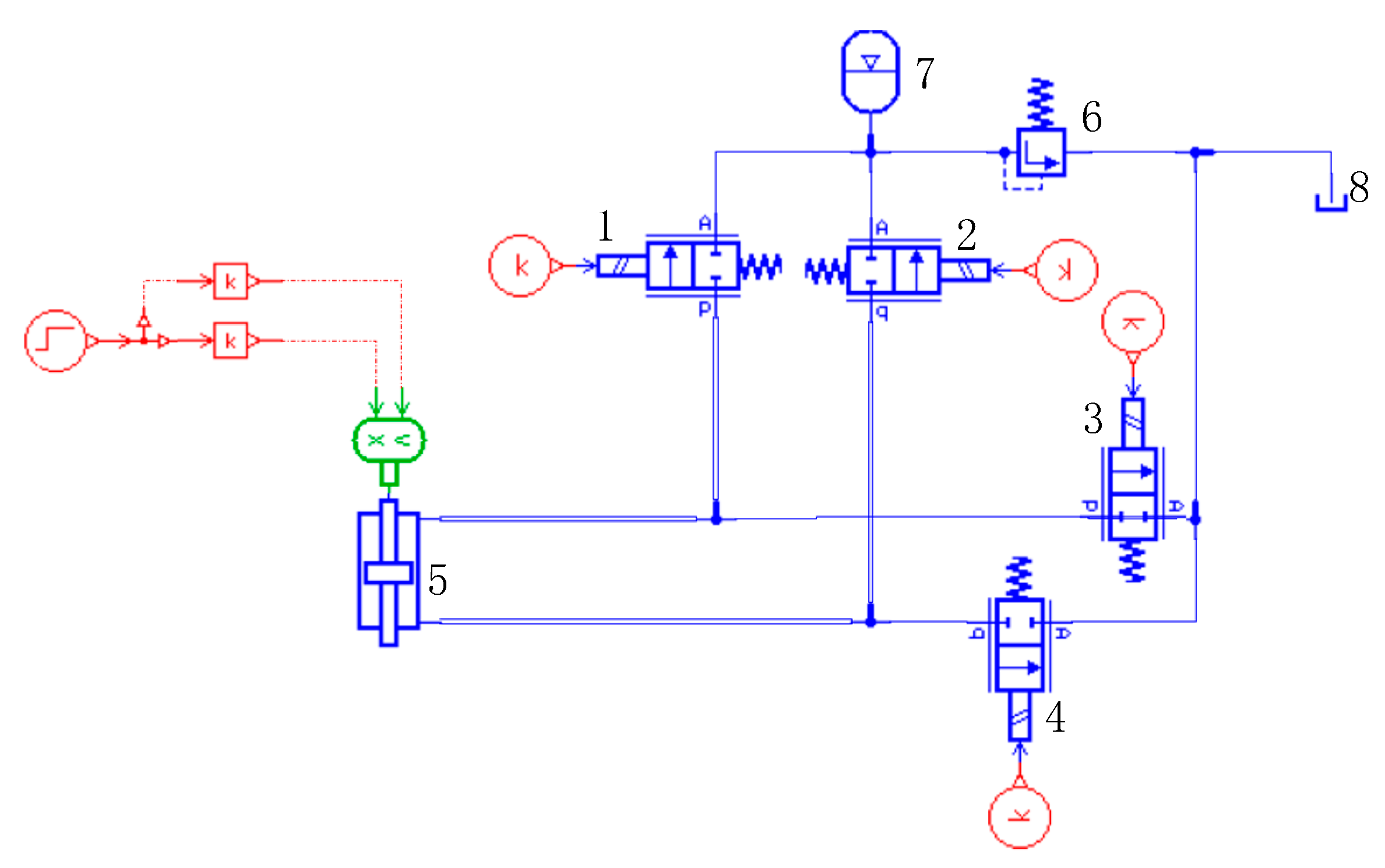
In order to test the EHA system, it is necessary to build a hydraulic loading system. The loading system in Figure 7 consists of an accumulator 7, an oil tank 8, four electromagnetic valves 1, 2, 3, and 4, and a piston-cylinder 5. The electromagnetic valve controls the flow path. The piston-cylinder of the loading system outputs load force to the EHA system. The accumulator provides energy to the loading system [36].
If electromagnetic valves 1 and 4 are opened and the electromagnetic valves 2 and 3 are closed, a spring-like load to the right will be output. While the electromagnetic valves 2 and 3 are opened and the electromagnetic valves 1 and 4 are closed, a spring-like load to the left will be output. The overflow pressure of the relief valve determines the upper limit of the spring-like force. Figure 8 shows the model of the hydraulic loading system in AMESIM and the component number in Figure 8 is the same as them in Figure 7.
The AMESIM-SIMULINK interface makes it possible to perform simulations with a combination of the hydraulic system and the motor system. According to the hydraulic device that was used in the experimental facility, the parameters of the hydraulic model are shown in Table 2.
The established hydraulic model uses the hydraulic library and the hydraulic component design (HCD) library in the AMESIM library. An orifice simulates the leakage of the pump. When the pressure difference is 4 bar, the leakage is 0.036 L/min. The pump elements with a leakage simulation can reflect the nonlinear characteristics caused by leakage in the experimental facility.
2.3. Experiment Facility
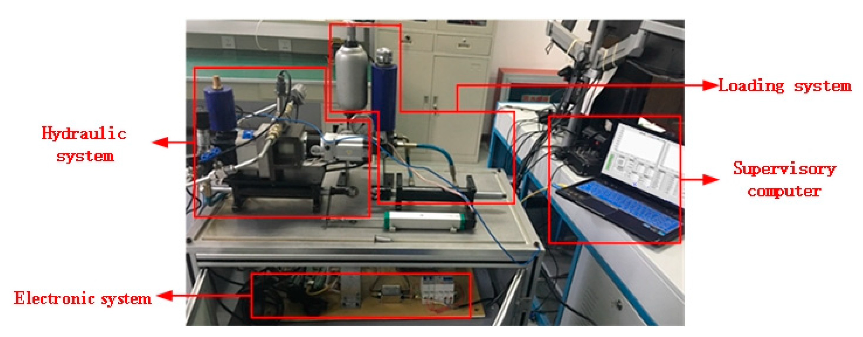
Based on the mathematical model of the EHA system, the experimental facility of the EHA was built. Figure 9 shows the structure of the experimental facility. It includes the motor control system shown in Figure 10, the hydraulic system shown in Figure 11, and the monitoring computer system shown in Figure 11.
Figure 10 demonstrates the motor control system facility, and the structure can be found in Figure 9.
The motor control system includes a power supply, an electronic controller, and an AC servo driver. The electronic controller is the core of the EHA system, which controls the motor’s speed and turn. The electronic chip TM4C1294NCPTD, a high-performance ARM Cortex-M based architecture on the controller, was used as the core of control. The chip provides an Ethernet communication function, enabling it to communicate with the monitoring computer through Ethernet, which makes data transmission faster and safer. The chip receives control data from the monitoring computer and the hydraulic system’s status parameters from sensors.
The hydraulic system consists of a motor, gear pump, double hydraulic chamber single rod piston cylinder, and a hydraulic lock. Figure 6 shows the order of connection of those components, and Figure 1 shows the details. The pressure sensors and the displacement sensors were set up in the system. The displacement sensor was connected parallel with the piston cylinder’s rod to measure the piston cylinder’s displacement output. Figure 11 shows the hydraulic system and the supervisory computer.
The loading system in Figure 11 consists of an accumulator, an oil tank, four magnetic valves and a piston cylinder. The magnetic valve controls the flow path, making the piston cylinder of the loading system move in the same or opposite direction as the piston cylinder of the hydraulic system. The accumulator provides energy to the loading system [36].
3. Analysis of the Stability and the Delay
3.1. Analysis of Stability
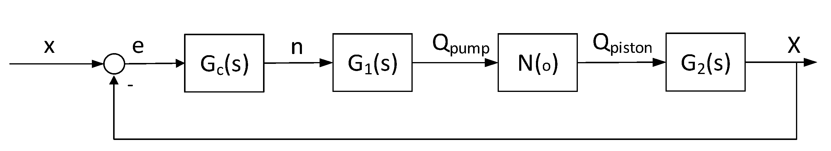
In Figure 12, is the transfer function of the controller, is the transfer function of the motor-pump system, is the transfer function that causes the delay, and is the transfer function of the piston cylinder. For single input single output models, the PID controller is widely used [37]. Therefore, we adopted the PID controller to analyze the stability of the closed-loop system.
Due to the hydraulic lock, the controller output was insufficient to overcome the leakage and the output displacement when the error was small. There was almost no overshoot in the system, so the differential link had little effect on the dynamic performance. So, the stability analysis of the closed-loop control system using the PI controller is analyzed. Assume that the controller is a PI controller.
Next, we need to analyze the transfer function that causes the delay . Figure 13 shows operating mode A that the piston-cylinder moves to the right.
As can be seen from Figure 13, the inlet of the piloted check valve A(PVA) is high pressure, and the inlet of the piloted check valve B (PVB) is low pressure. The piston-cylinder starts to move when the PVA and the PVB are both open and the hydraulic pressure force overcomes the damping-like load force, which means the piston-cylinder would move while:
while the piston-cylinder is moving, it is clear that:
So, the piston-cylinder would move while Equation (19) is satisfied. When Equation (19) is satisfied, it’s easy to know that Equation (17) must be satisfied, which means the influence of the PVB can be ignored.
All of the factors that lead to the delay can be seen as a transfer function . When the rotation direction of the motor changes, the system turns into mode B, and the integral of the flow rate should reset. This means that the output of the transfer function is:
Equation (20) indicates that can be seen as a switch, and the output of it is positive semidefinite.
In operating mode A, has been analyzed. In operating mode B, the position error is negative, so are the motor’s rotation speed , the flow rate out of the pump , and the flow rate inlet the piston-cylinder . So, the transfer function combining the mode A and the mode B can be expressed as:
and are linear transfer functions, which can be expressed as
so, the characteristic Equation of the closed-loop system is
Assuming that the motor with the controller is a simple inertial component with the nonlinear factor removed. The pump is a proportional component with the nonlinear factor removed. The piston-cylinder is an integral component with the nonlinear factor removed. So, in , the transfer function of the system is
and the characteristic Equations of the closed-loop system can be written as
The Rouse criterion shows that the system is stable only if . Due to the transfer function , when or is not large enough, the output is 0, making the error not 0. The integral control will lead to the accumulation of errors. It may lead to instability and oscillation. To satisfy the Rouse criterion, and to avoid the accumulation of errors, let us assume , and the zero and the pole of the transfer function could cancel at , and the other pole is
if is not big enough, the motor’s rotational speed is low when the error is small, and the check valve opening is almost zero. This means and , thus the system is stable and it will not oscillate. If is too big, the rotation output is high even when the error is small. It means and , thus the system is stable but it will oscillate.
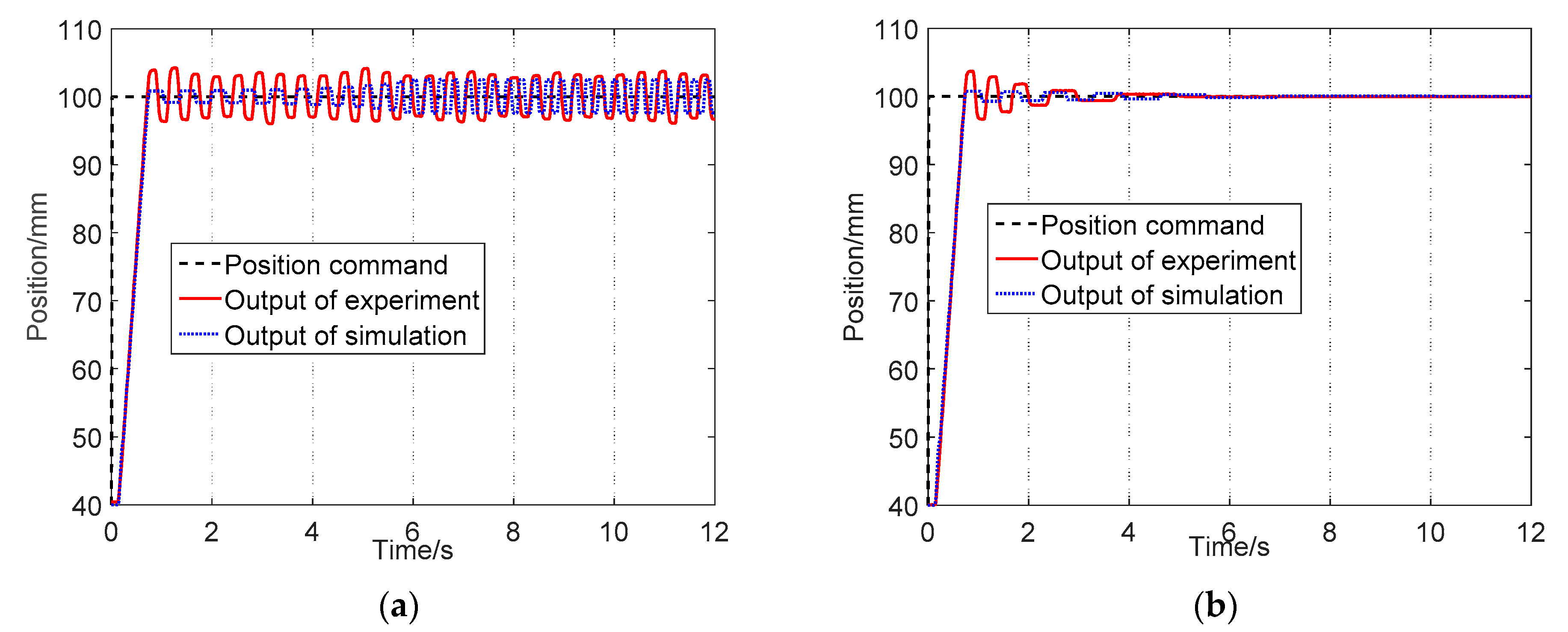
Figure 14 shows the closed-loop step control simulation and the experimental result with the substantial coefficient proportional controller.
In Figure 14a, the proportional coefficient is as large as 160, and the system has apparent oscillation. In Figure 14b, the proportional coefficient is as large as 120, but the oscillation of the system is eventually suppressed. The simulation and the experimental results show the same stability characteristics. Since the piston cylinder is an integral component, if there was no hydraulic lock and the proportional coefficient was appropriate, the steady-state error would be eliminated. The oscillation of the system is due to the larger proportional coefficient. Equation (29) shows that if , the oscillation occurs, and if , the oscillation suppresses. The pressure between the piloted check valve’s input and output is essential to . Due to leakage, when the pump speed is not high enough, . When the proportional coefficient is small, the pump speed is low and . So, the addition of the hydraulic lock reduces the oscillation of the system.
Therefore, the appropriate proportional coefficient is essential. The steady-state error is required to be within 1 mm to meet the requirements of position control in MEA, and corresponding to a 1 mm error, the proportional coefficient is 20. When the pump speed is 20 RPM, the output displacement of the piston-cylinder can be ensured, although there is a delay of 4.5 s. If the pump speed is lower than 20 RPM, it cannot be guaranteed that there is a position output, which leads to a steady-state error of approximately 1 mm.
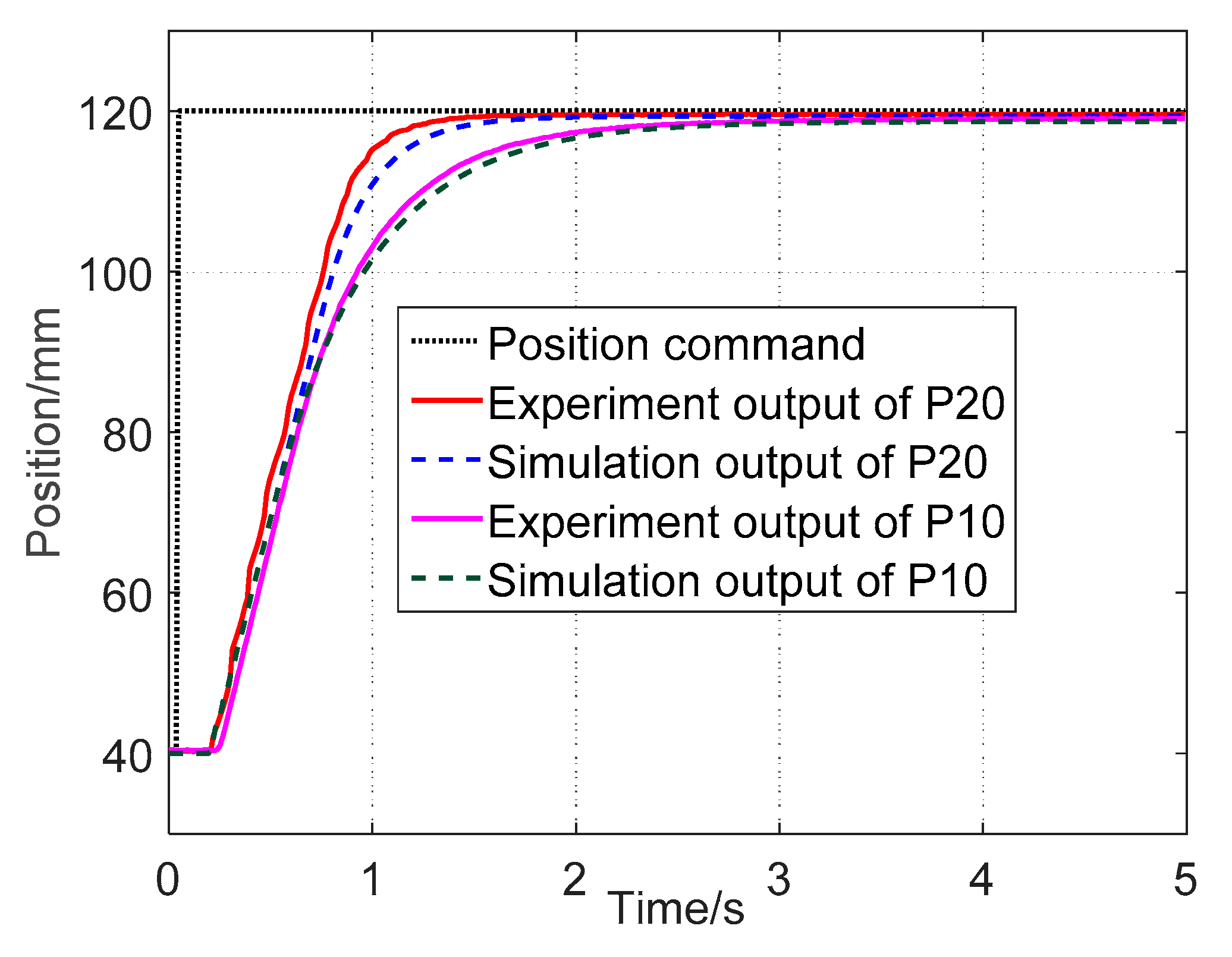
Figure 15 shows the closed-loop simulation and the experimental results of step control of position when the proportional coefficient is 10 and 20. The results show that with the proportional coefficients 10 and 20, the delay was approximately 0.15 s, and the rising times were 1 s and 1.5 s, respectively. At the same time, the simulation and the experimental results are consistent in both the dynamic and the steady-state, and the error of the dynamic state was less than 3%, while the error of the steady-state was less than 0.5%. The proportional coefficient had a noticeable influence on the dynamic characteristics of step control. The delay was the same because the controller output saturation was 500 RPM. The steady-state error was approximately 1.2 mm with the proportional coefficient 10. When the proportional coefficient was 20, the steady-state error was suppressed, which satisfied the analysis above. Due to the small proportional coefficient, which leads , the oscillation of the system was also suppressed.
The BHL-EHA system comprises the proportional component, inertial component, delay component, and integral component. As the inertial component was the motor with a closed-loop speed controller, the time parameter of the inertial component was small, which is shown in Figure 4. So, in the low-frequency range, the open-loop frequency characteristics of BHL-EHA were mainly affected by the proportion link, the delay component, and the integral link. However, the open-loop performance of the BHL-EHA system shown in Figure 16 was low. This was due to the maximum speed of the pump being limited to 500 RPM, so the performance of the BHL-EHA system was low.
Figure 16 is the open-loop sinusoidal simulation and the experimental results, and in the open-loop control, the input was the speed of the motor and the output was the position of the piston. The figure shows that the simulation results are consistent with the experimental results, which further shows the accuracy of the simulation model. There was a delay when the speed of the motor was 0, that is when the phase of sinusoidal speed was 0 or −180°. It can be seen in the figure that the output of the piston position is a cosine wave, which means that the piston-cylinder was an integral component and the integral link had the most influence. When the frequency changed, the phase lag hardly changed. The phase lag was approximately −90°, which was the same as the phase lag of the integral link. The delay did not affect the phase.
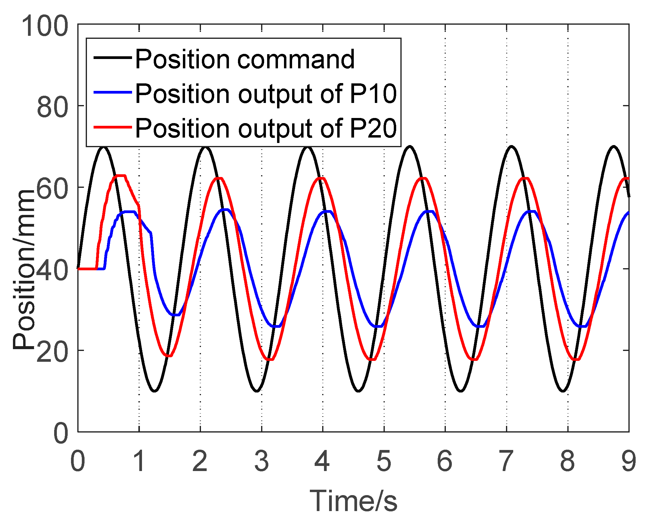
Figure 17 shows the closed-loop simulation of the sinusoidal position output control with different proportional coefficients. The lower the frequency of the sinusoidal control signal, the better were the control effects. The higher the proportional coefficient, the better were the control results. On the one hand, increasing the proportional coefficient could increase the cut-off frequency of the system. On the other hand, when the motor commutated, the delay influenced the sinusoidal position output control. The delay was smaller when the proportional coefficient was larger at the same error.
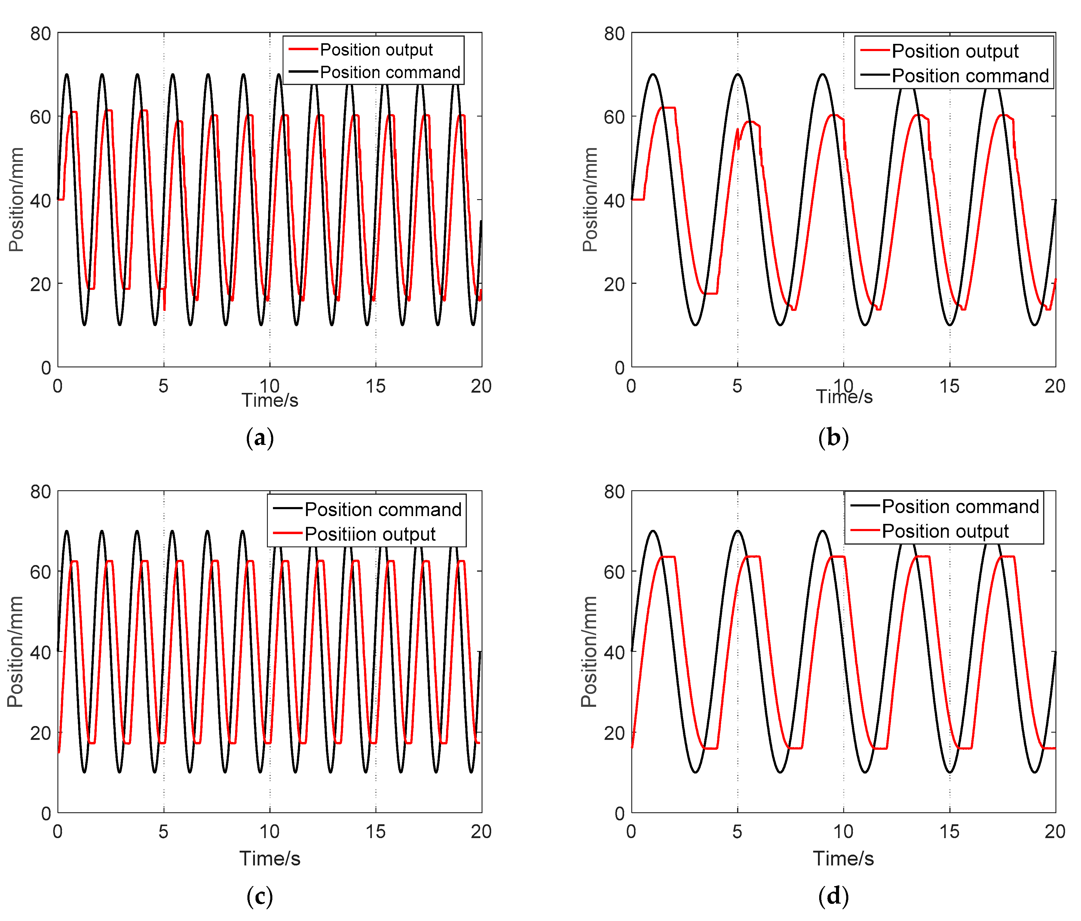
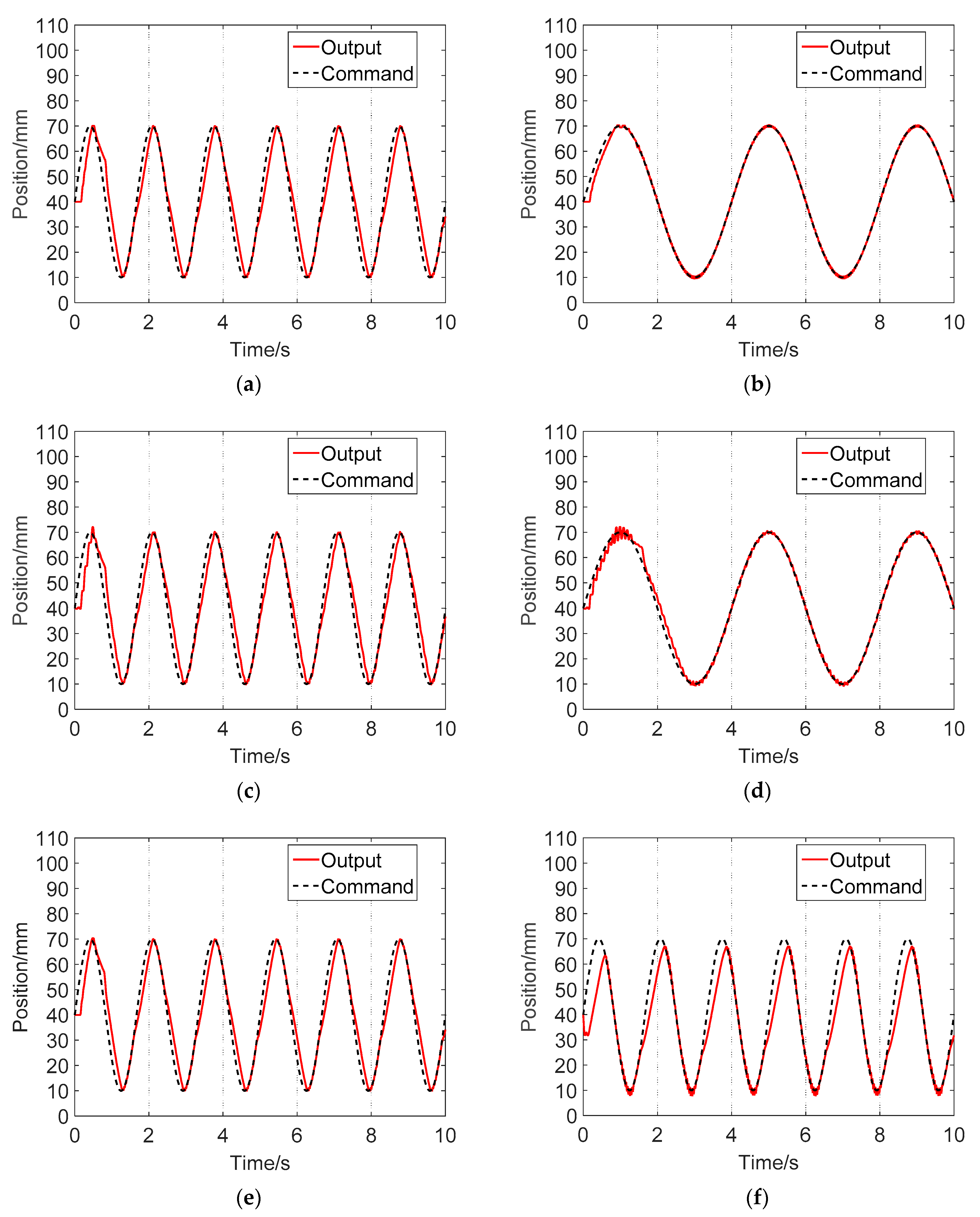
Figure 18a shows the simulation results with a proportional coefficient of 20 and Figure 18b with a proportional coefficient of 10. Figure 18c shows the experimental results with a proportional coefficient of 20 and Figure 18d with a proportional coefficient of 10. It can be seen from Figure 18 that the experimental results are consistent with the simulation results. Figure 18a,c show that when the frequency of the input command was 0.63 Hz, the amplitude of output displacement was approximately 40 mm, which was approximately of the input that was 60 mm. Moreover, when the proportional coefficient was 10, the closed-loop system’s gain margin was 0.25 Hz, which can be seen in Figure 18b,d.
It indicates that the cut-off frequency of the closed-loop system with a proportional coefficient of 20 was 0.6 Hz, while the cut-off frequency was 0.25 Hz when the proportional coefficient was 10.
Table 3 shows the cut-off frequency of the closed-loop system in different proportional coefficients by simulation. It can be seen that with the increase of the proportional coefficient, the cut-off frequency increased. However, with the increase of the proportional coefficient, the cut-off frequency did not increase significantly because the maximum output speed was limited to 500 RPM in this study.
3.2. Analysis of the Delay
In the low-speed open-loop experiment, the delay occurred. Figure 19 shows the simulation results of the simulation and the experiment, and the motor speed is 20 RPM to make the delay obvious.
As can be seen from Figure 19, The results of the simulation and the experiment are consistent. When the motor speed was low, there was a significant delay in the pressure and the position output. The hydraulic lock delayed the pressure output. When the differential pressure output was enough to overcome the load force, the position began to output. When the speed was only 20 RPM, the delay of the position output was up to 4.5 s, which had a very adverse impact on the position control of EHA. Therefore, it is necessary to study the causes of the delay.
The fluid resistance and the capacitance had a significant influence on the dynamic characteristic of the system. Since the characteristics of the pump and the piston-cylinder are well known, it is not introduced and analyzed in detail.
The fluid resistance and the capacitance are defined as:
The diameter, roughness, and flow of the pipe are related to , and is related to the elasticity modulus and the fluid’s compressibility.
According to the definition of fluid resistance and capacity, the pressure changes in the pipeline can be expressed as:
The pipe volume is V and is the effective bulk modulus of the pipe/fluid combination.
Combined with the analysis of Figure 13 and Equations (15)–(21), it is clear that the delay was related to the fluid flow Q, fluid capacitance , crack pressure of PVA , and output pressure of PVA . The output pressure of PVA was affected by the load force and the friction. The delay was determined by the flow-time integral. The output of the was 0 until the flow-time integral was greater than . With the pump and the piston cylinder’s leakage taken into account, the piston-cylinder could not move if the rotation speed was not high enough. According to the analysis above, the delay was considerable when the rotation speed of the motor was very low.
Therefore, in the model established in Section 2, the length and the diameter as well as Young’s modulus of the pipe would influence the delay of the system. The piston-cylinder diameter and the rod determine the movement rate of the piston rod at the same flow rate. The diameter of the piston-cylinder also determines the pressure difference under the same load force. Therefore, the parameters of the piston-cylinder element also influences the delay of the system. The use of the HCD element in the simulation can fully reflect the valve’s poppet position and provide a basis for analyzing the delay. At the same time, the Reynolds number and the flow coefficient of the hydraulic lock can also be obtained.
Figure 20 shows the poppet position of the hydraulic lock, the flow area, and the pressure at the input of the hydraulic lock. Since the flow area and the poppet position are of the same order of magnitude, the left y-axis shows both the flow area and the poppet position in Figure 20.
In the beginning, the poppet position changed to −0.2 mm, which was because of the spool displacement caused by the spring preload. With the increase of input pressure, the pressure generated by overcame the spring preload. When the valve poppet position was greater than 0, the valve opened.
As shown in Figure 20, the delay of the poppet position is almost the same as the delay of the flow area. The delay is approximately 3 s. Figure 19 shows that the pressure at the input of the piston-cylinder also started to increase at 3 s.
At approximately 4.2 s, the pressure at the input of the piston-cylinder reached 0.6 bar, and the piston-cylinder started to move. At the same time, the input pressure of the hydraulic lock reached 4.6 bar. It satisfied the condition that Equation (19) expresses.
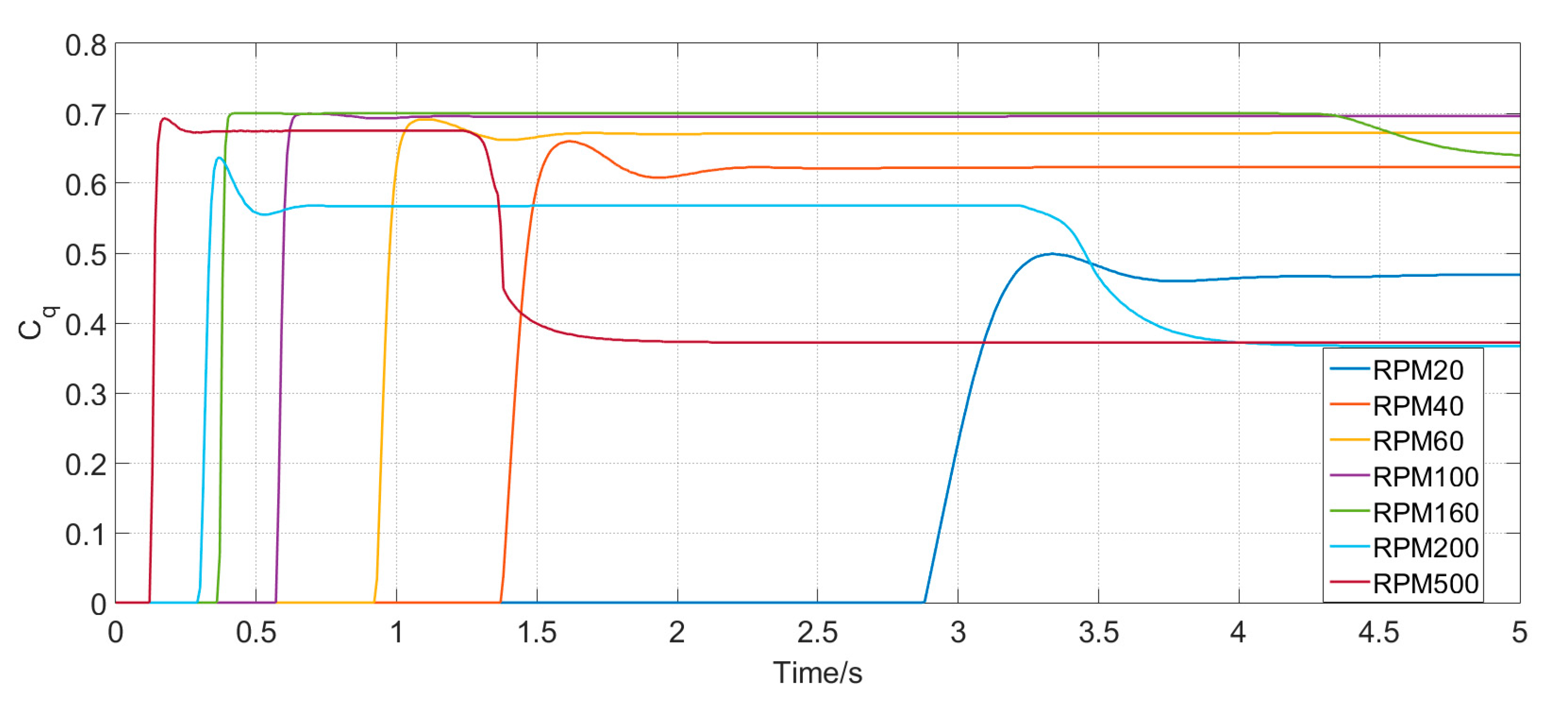
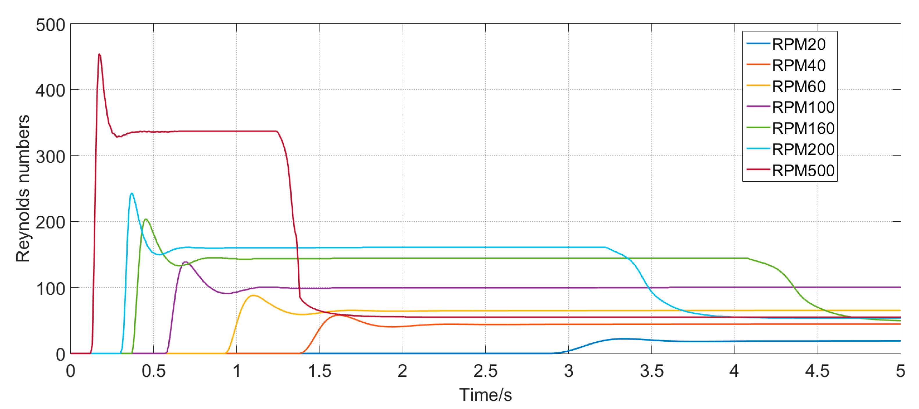
As the flow coefficient is a function of the Reynolds number , and is related to the velocity and the hydraulic diameter, so and are different at different pump speeds. Figure 21 shows flow coefficients and Figure 22 shows the Reynolds numbers of the hydraulic lock at pump speeds of 20 RPM, 40 RPM, 100 RPM, 160 RPM, 200 RPM, and 500 RPM.
As shown in Figure 22, the Reynolds number is larger at a higher speed. The maximum Reynolds number is 450. When the piston-cylinder started to move, the opening area and the flow rate of the hydraulic lock remained stable, and the Reynolds number also remained stable. At 160 RPM and above, the Reynolds number suddenly decreased and it soon remained stable because the flow rate decreased due to the movement of the piston-cylinder to the limit position. When the piston-cylinder reached the limit position, there was still a low flow rate due to leakage, so the Reynolds number will not be 0.
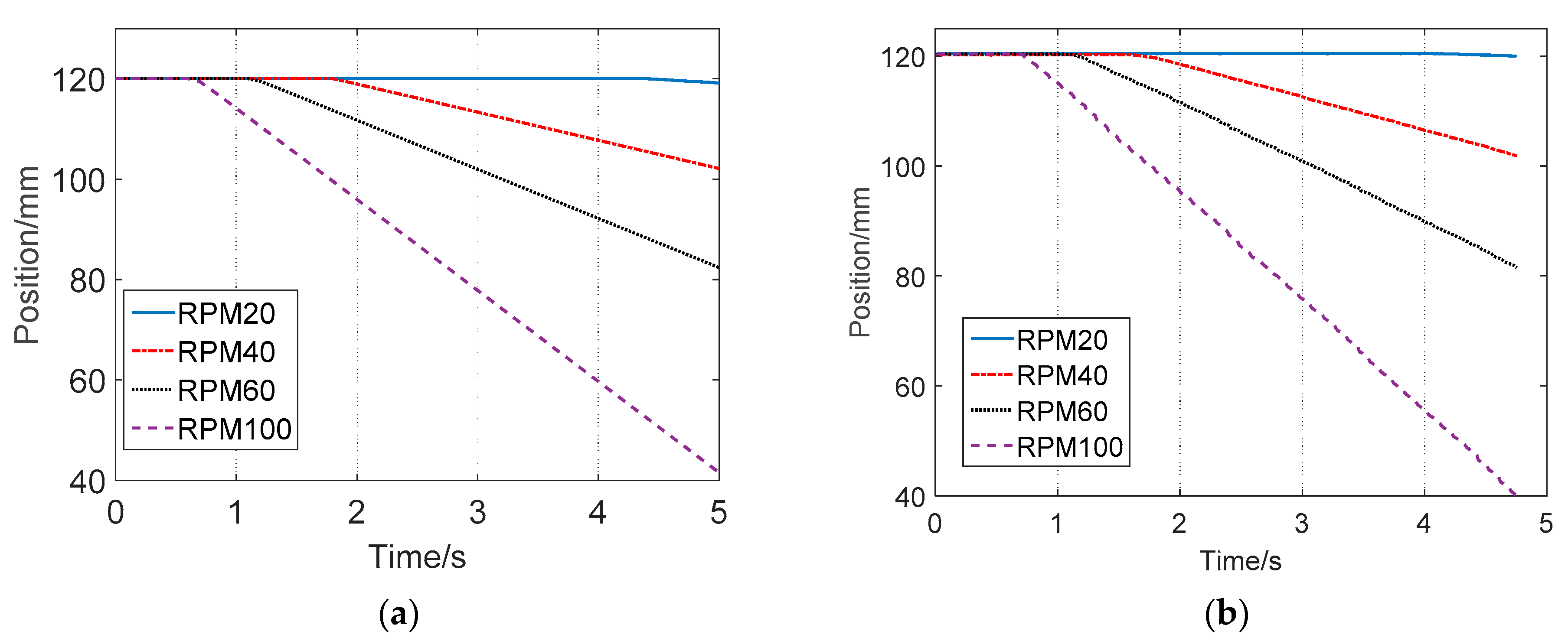
Figure 23 shows the simulation and the experimental results of the position output in the open-loop control at a different rotational speed.
It can be seen from Figure 23 that when the pump speed was low to 20 RPM, the position started to change at 4.2 s. When the pump speed was 40 RPM, 60 RPM, or 100 RPM, the position started to change at 1.7 s, 1.2 s, and 0.7 s, respectively. The larger the flow rate, the faster the pressure change, which resulted in a lower delay.
The delay of the simulation and the experiment can nearly agree. Table 4 shows more details about the opening time of the hydraulic lock, the rising time of the pressure difference of the piston-cylinder, and the position delay. The detailed data comparison between the experiment and the simulation is also shown in Table 4.
Table 4 indicates that the sum of the opening time of the hydraulic lock and the rising time of the pressure difference was equal to the delay of the position output. The results conform to the analysis of the delay. The hydraulic lock started to open when Equation (21) was satisfied. The product of the pump speed and the delay of position was approximately 65 to 85. This product was equivalent to the integral of flow over time. The difference of the product at different pump speeds may have been due to leakage, which needs to be studied in the future. At the same time, Table 3 also shows that the experimental results are consistent with the simulation results, and the delay length of the two is almost the same.
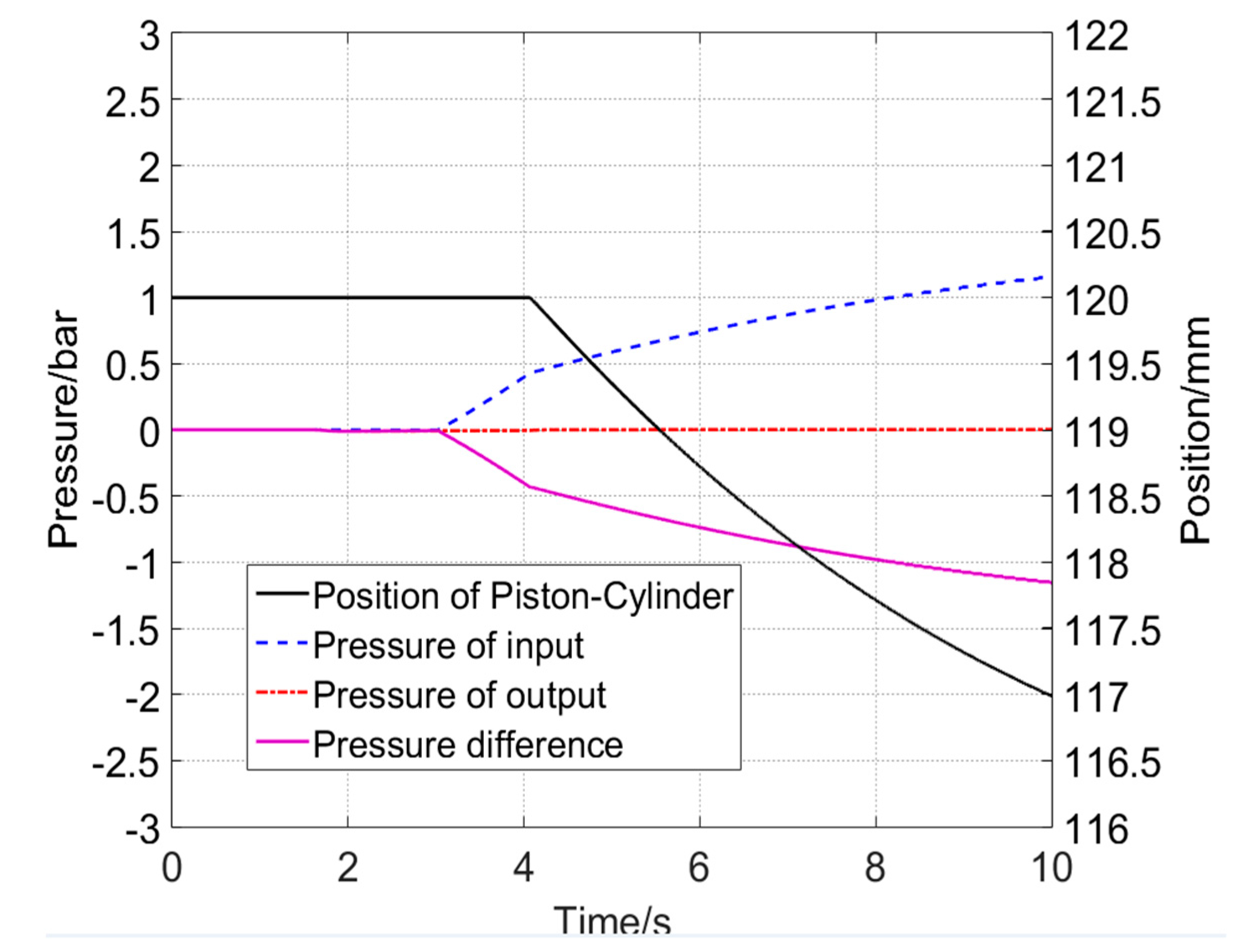
Figure 24 shows the position, inlet pressure, and outlet pressure of the piston-cylinder under spring-like loads at 20 RPM.
As shown in Figure 24, the opening time of the hydraulic lock is almost unaffected during spring-like loading. Hence, the delay of the position output of the piston-cylinder was almost unchanged. With the movement of the piston-cylinder, the pressure difference increased gradually. With the increase of the pressure difference, the movement speed of the piston-cylinder decreased gradually due to the leakage of the pump and the piston-cylinder. The spring-like loads will affect the dynamic characteristics of the position output, but it will not affect the delay. However, the damping-like load will affect the delay. That is because the piston-cylinder output hydraulic pressure must be greater than the damping (such as friction resistance) before it starts to move, while the spring-like load begins to increase after it starts to move.
It is difficult to achieve a quantitative analysis of the delay in the frequency domain caused by the hydraulic lock. Let’s define a factor number
where is the amplitude of the pump’s speed, and is the input frequency. When , as Table 3 shows, we solve for . The factor number indicates the system’s amplitude attenuation influenced by the hydraulic lock, and indicates the actual delay. If , the output is always 0 because the delay is bigger than the input frequency. The condition is the same as the condition that the factor number is less than 65. When , . Assume that
as grows larger, the influence of the hydraulic lock grows smaller. However, the minimum delay was 0.15 s when using the experimental equipment described in Chapter 2. That is because the maximum speed of the pump was 500 RPM, which means . This means that when the frequency is equal to 6.67 Hz, the hydraulic lock cannot be opened, which will also lead the output of the open-loop system to become 0.
At the same time, as shown in Figure 15 with its analysis, the spring-like load does not affect the delay. However, the damping-like load will affect the delay time. Therefore, when the damping-like load (such as friction) changes, the limit value of is not 65.
More generally, is the current pump rotation speed and let
According to the ideal pump flow equation, Equations (16) and (21), when the hydraulic cylinder starts to move, the delay time and have the following relationship
where is the pump displacement. Equations (32) and (33) show that once the rotational speed is determined, the delay time is determined. Equations (32) and (33) can be extended to all EHA systems with hydraulic locks. If the EHA system does not have the hydraulic lock, remove and in Equation (33).
4. Delay Compensation Control
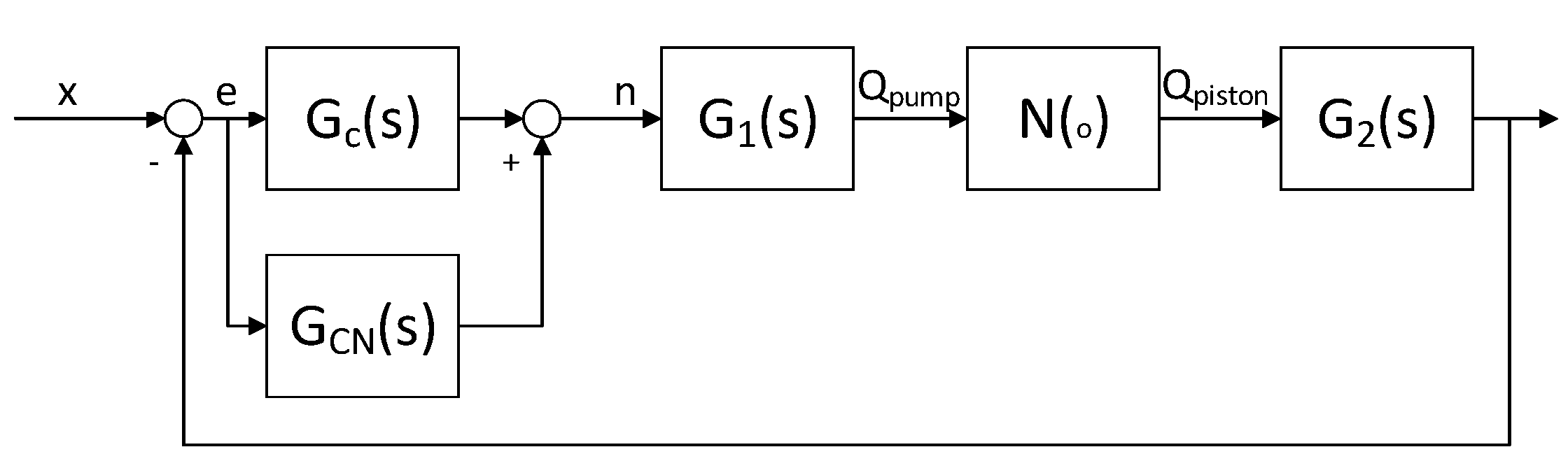
As Equations (32) and (33) show, once the hydraulic lock characteristics, pump characteristics, pipeline characteristics, and load are determined, there is a one-to-one correspondence between rotational speed and delay time. A delay compensation control method is used to minimize the delay. Figure 25 shows the transfer function diagram.
The feedforward control method can also eliminate the delay and the damping of a system with the transfer function . So, the delay compensation controller can be designed. When , is enabled and let , then
where is the feedforward values. When , it means the operation mode changes from A to B. When the operation mode changes, the controller output commands to the EHA system to minimize the delay. Once the maximum speed is determined, the minimum delay is determined according to Equations (32) and (33). In this case, the delay compensation controller can be constructed according to and .
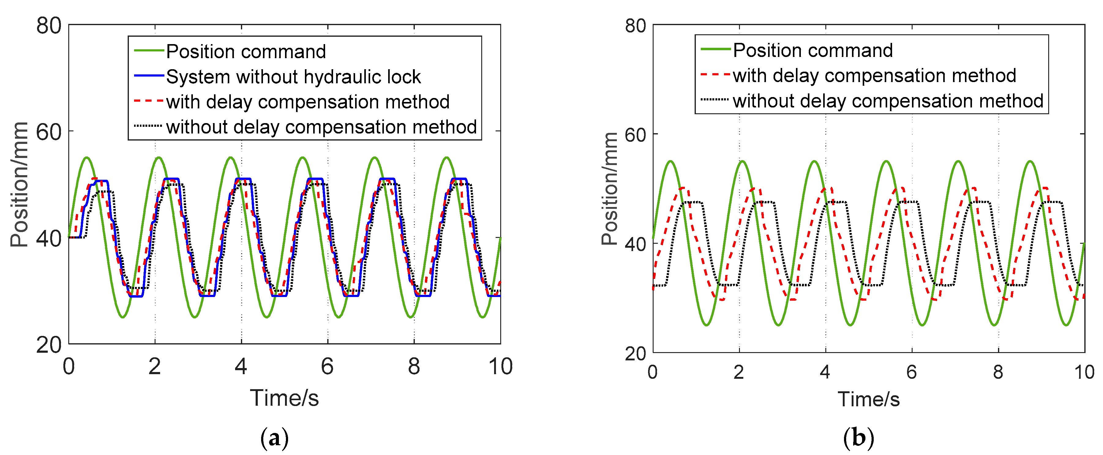
Figure 26a shows the simulation results of the EHA system with a hydraulic lock using the delay compensation control method with , the EHA system with the hydraulic lock not using the delay compensation control method, and the EHA system without the hydraulic lock using the PI control method. Figure 26b shows the experimental results of the EHA system with the hydraulic lock using the delay compensation control method with , and the EHA system without the hydraulic lock using the PI control method. As the hydraulic lock is placed in the pump, the experimental results lack comparison with the EHA system without the hydraulic lock. The input signal is a 15 mm amplitude, 40 mm mean level, and 0.6 Hz frequency sine wave. And the proportional and integral coefficients are . The result shows that using the delay compensation control method can reduce the influence of the hydraulic lock. In more detail, the delay occurs when the derivative of the position . A delay compensation control command is outputted to ensure the delay reaches the minimum value of . In this paper, and s, which is analyzed in Section 3, and it can be obtained by Equations (32) and (33). It can be seen from Figure 26 that the position output amplitude of the system using the delay compensation control method is very closed to the system without a hydraulic lock, which in the simulation was approximately 10.5 mm and in the experiment it was approximately 10.08 mm. In the BHL-EHA system, when the position command is at the stagnation point of the sine wave, if the delay compensation control method is not used, there will be a delay of approximately 0.35 s, which resulted in the amplitude of only 8 mm in the simulation and only 7.6 mm in the experiment. After using the controller, the amplitude error of the system was reduced from 49.3% to 32.8%. The phase lag was approximately 5° compared with the system that uses the delay compensation control method in the experiment.
Figure 27a,b show the simulation results using the delay compensation control method, with the same command of Figure 18a and Figure 18b, respectively. In Figure 27a, and in Figure 27b, . Figure 27c,d show the results when the sine load is applied, and the load is 10 Hz, 20 bar. Figure 27e shows the result of using the same command and control parameters as (a) when the temperature is 0 °C. Figure 27e shows the result of using the same command and control parameters as Figure 27a when the load of 5 MPa is applied.
Comparing Figure 18 and Figure 27, the delay compensation control method combined with feedforward control achieves excellent control results. When the sinusoidal input is applied, the output position tracks the input very well. The amplitude error is within 3% and the phase lag is 0°. Compared with the method without feedforward, this method reduces the amplitude error by 29.8% and corrects the phase lag of 10°. Compared with the normal PID controller, this method reduces the amplitude error by 46.3% and it corrects the phase lag of 15°.
It can also be seen from Figure 27e that the change of temperature and load has little effect on the delay compensation control method. Periodically changing load will cause a slight jitter of position output, but it will not affect the delay. According to Equations (32) and (33), the temperature change will change the effective bulk modulus , thus changing the delay . However, the change caused by is very small, so the control performance is almost not influenced, which ensures the robustness of the controller.
Figure 27f shows the result of the delay compensation control method when 5 MPa load is applied. According to Equations (32) and (33), with unchanged, the increase of the damping-like load will increase . As a result, the load increases the delay. In the positive half cycle of the sine command, the load direction is opposite to the command. In the negative half cycle of the sine command, the load direction is the same as the command. Therefore, the positive half cycle tracking performance is weakened, while the negative half cycle tracking performance is enhanced. However, compared with the result without the compensation control method (as shown in Figure 19, even without load), it can achieve a good control effect. However, to improve the control effect, the controller should be modified according to Equation (33) when the load changes
where is the delay time after adding the opposite load, calculated according to Equations (32) and (33) and is the delay time after adding the aiding load. Figure 28 shows the control effect under a 5 MPa unidirectional load after the controller parameters are modified.
By comparing Figure 28 with Figure 27f, although Figure 27f shows good robustness of the controller, a better control effect can be achieved in the positive half cycle of the sine command after controller parameter correction.
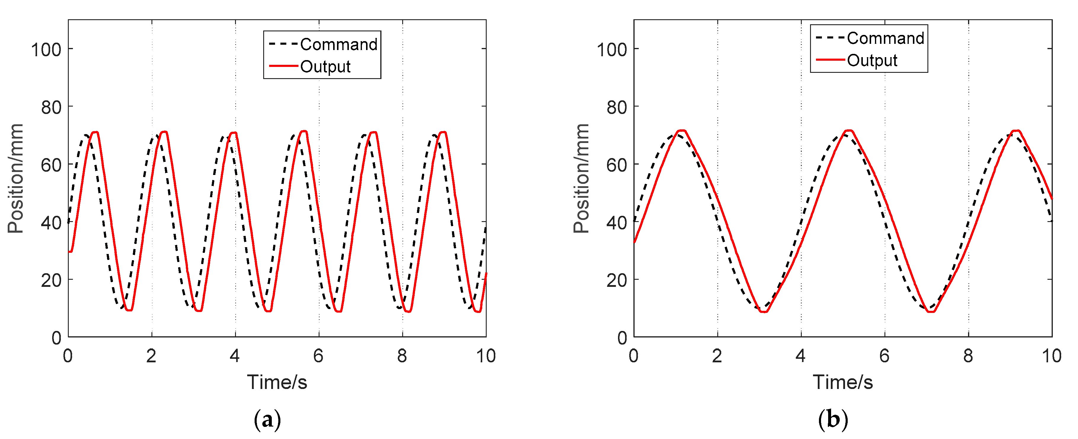
Figure 29a,b show the experimental results using the delay compensation control method, with the same command of Figure 18a,b, respectively. In Figure 29a, the proportional coefficient is 20 and the , while in Figure 29b, the proportional coefficient is 10 and the . The experimental results show that the delay compensation control method can strengthen the tracking performance of the BHL-EHA system and completely compensate for the amplitude difference of sinusoidal control; the amplitude of the position output is even 3% higher than the command amplitude.
Comparing Figure 29 with Figure 27, the experimental results are inconsistent with the simulation results that the phase lag is 10°, which may be caused by the dead zone of the actual experimental facility. Although there is a phase lag in the actual experimental results, compared with the control results without the delay compensation control (as shown in Figure 18), the phase lag is compensated.
5. Conclusions
Compared with the traditional hydraulic system, the EHA system has a higher energy density. However, to ensure that the position remains unchanged when the load changes, the motor needs to work continuously. To save more energy, the hydraulic lock is used to realize the internal contracting brake function of the EHA system. But the BHL-EHA system has a delay, which leads to a dynamic response error. In many other studies, the phenomenon of a delay in EHA is not considered sufficiently [20,21,22], but the delay of the BHL-EHA system needs to be analyzed. In this paper, the delay of the BHL-EHA system is studied, and the following conclusions are obtained:
- The delay of the BHL-EHA is demonstrated and analyzed. The delay is related to the fluid flow Q, the fluid capacitance , the hydraulic lock’s crack pressure and the load . More generally, the factors affecting the delay are explained by the proposed Equations (32) and (33);
- The stability of a closed-loop control using the PI controller is investigated. It proves that the system is stable only if . However, if the proportional coefficient is too large, the system has apparent oscillation due to the characteristic of the PI controller;
- A delay compensation control method is proposed to minimize the delay caused by the hydraulic lock. The results show that the delay compensation control method can minimize the delay of the BHL-EHA position output. In the simulation, the amplitude error was within 3% and the phase lag was 0°. Compared with the normal PID controller, this method reduces the amplitude error by 46.3% and it corrects the phase lag of 15°. In the experiment, the delay compensation control method could strengthen the tracking performance, the amplitude of the position output was even 3% higher than the amplitude of command, but there was a phase lag of 10°, which may have been caused by the dead zone of the actual experimental facility.
The delay compensation control method can be used in industrial application, as long as the parameters of the EHA system that Equations (32) and (33) need can be determined. However, the parameters of the EHA system would change with long working hours, which is the major obstacle that needs to be overcome.
However, this paper also has some limitations. The delay in the EHA system is inevitable, especially after using the hydraulic lock. Although this paper analyzes the causes of the delay and it proposes a delay compensation control method, the proposed method depends on the determined load. In future research, the control method should have the ability to adapt to load changes.
Author Contributions
Conceptualization, J.Z.; Data curation, J.Z.; Formal analysis, J.Z. and Y.Y.; Funding acquisition, T.Z.; Investigation, X.Z.; Methodology, J.Z. and X.Z.; Project administration, T.Z.; Resources, J.Z.; Software, J.Z. and L.L.; Supervision, T.Z.; Validation, J.Z.; Visualization, L.L.; Writing—original draft, J.Z.; Writing—review & editing, J.Z., L.L., X.Z. and Y.Y. All authors have read and agreed to the published version of the manuscript.
Funding
This work received the financial support of the Postgraduate Research & Practice Innovation Program of Jiangsu Province for the research (project number: KYCX18_0316). This work was supported by the National Natural Science Foundation of China (grant number: 51976089).
Institutional Review Board Statement
Not applicable.
Informed Consent Statement
Not applicable.
Acknowledgments
The authors thank Tian-Hong Zhang for his guidance on this paper and the help of students from our research office. In particular, we thank other researchers for their illuminating work in the EHA study.
Conflicts of Interest
The authors declare no conflict of interest.
References
- Rosero, J.A.; Ortega, J.A.; Aldabas, E.; Romeral, L. Moving Towards a more Electric Aircraft. IEEE Aerosp. Electron. Syst. Mag. 2007, 22, 3–10. [Google Scholar] [CrossRef] [Green Version]
- Croke, S.; Herrneschmidt, J. More electric initiative-power-by-wire actuation alternatives. In Proceedings of the National Aerospace and Electrics Conference (NAECON’94), Dayton, OH, USA, 23–27 May 1994; pp. 1338–1346. [Google Scholar]
- Naayagi, R.T. A review of more electric aircraft technology. In Proceedings of the 2013 International Conference on Energy Efficient Technologies for Sustainability(ICEETS), Nagercoil, India, 10–12 April 2013; pp. 750–753. [Google Scholar]
- Emadi, K.; Ehani, M. Aircraft power systems: Technology, state of the art, and future trends. IEEE Aerosp. Electron. Syst. Mag. 2000, 15, 28–32. [Google Scholar] [CrossRef]
- Botten, S.L.; Whitley, C.R.; King, A.D. Flight control actuation technology for next-generation all-electric aircraft. Technol. Rev. J. 2000, 8, 55–68. [Google Scholar]
- Huang, X.; Gerada, C.; Goodman, A.; Bradley, K.; Zhang, H.; Fang, Y. A brushless DC motor design for an aircraft electro-hydraulic actuation system. In Proceedings of the 2011 IEEE International Electric Machines & Drives Conference(IEMDC), Niagara Falls, ON, Canada, 15–18 May 2011; pp. 1153–1159. [Google Scholar]
- Wheeler, P.W.; Clare, J.C.; Trentin, A.; Bozhko, S. An overview of the more electrical aircraft. Proc. Inst. Mech. Eng. Part G J. Aerosp. Eng. 2012, 227, 578–1163. [Google Scholar] [CrossRef]
- AbdElhafez, A.A.; Forsyth, A.J. A review of more-electric aircraft. In Proceedings of the 13th International Conference on Aerospace Sciences and Aviation Technology (ASAT-13), Cairo, Egypt, 26–28 May 2009; pp. 1–13. [Google Scholar]
- Habibi, S.; Goldenberg, A. Design of a new high-performance electro-hydraulic actuator. In Proceedings of the 1999 IEEE/ASME International Conference on Advanced Intelligent Mechatronics (Cat. No.99TH8399), Atlanta, GA, USA, 19–23 September 1999; pp. 158–164. [Google Scholar]
- Manring, N.D.; Luecke, G.R. Modeling and designing a hydrostatic transmission with a fixed-displacement motor. J. Dyn. Syst. 1998, 120, 45–50. [Google Scholar] [CrossRef] [Green Version]
- Boldea, I.; Nasar, S.A. Linear Electric Actuators and Generators. IEEE Trans. Energy Convers. 1999, 14, 712–717. [Google Scholar] [CrossRef]
- Karpenko, M.; Sepehri, N. Hardware-in-the-loop simulator for research on fault tolerant control of electrohydraulic actuators in a flight control application. Mechatronics 2009, 19, 1067–1077. [Google Scholar] [CrossRef]
- Navarro, R. Performance of an Electro-Hydrostatic Actuator on the F-18 Systems Research Aircraft; National Aeronautics and Space Administration, Dryden Flight Research Center: Edwards, CA, USA, 1997; Volume 206224, pp. 1–37.
- Gao, B.; Fu, Y.; Zhongcai, P. Research of the servo pump’s electrically driven variable displacement mechanism. In Proceedings of the IEEE International Conference on Mechatronics and Automation, Niagara Falls, ON, Canada, 29 July–1 August 2005; pp. 2130–2133. [Google Scholar]
- Nawaz, M.H.; Yu, L.; Liu, H.; Rehman, W.U. Analytical method for fault detection & isolation in electro-hydrostatic actuator using bond graph modeling. In Proceedings of the 14th International Bhurban Conference on Applied Sciences and Technology (IBCAST), Islamabad, Pakistan, 10–14 January 2017; pp. 312–317. [Google Scholar]
- Rongjie, K.; Zongxia, J.; Shaoping, W.; Lisha, C. Design and Simulation of Electro-hydrostatic Actuator with a Built-in Power Regulator. Chin. J. Aeronaut. 2009, 22, 700–706. [Google Scholar] [CrossRef] [Green Version]
- Kopp, J.D.; Neal, T.P. Tandem Electro Hydrostatic Actuator. U.S. Patent 20040163386 A1, 16 November 2004. [Google Scholar]
- Sweeney, T.; Kubinski, P.T.; Anderson, D.J. Electro-Hydraulic Actuator Mounting. U.S. Patent 8161742 B2, 24 April 2012. [Google Scholar]
- Olson, M.; Prazak, J. Electro-Hydraulic Actuator. U.S. Patent 20110289912 A1, 1 December 2011. [Google Scholar]
- Altare, G.; Vacca, A. A design solution for efficient and compact electro-hydraulic actuators. In Proceedings of the 2nd International Conference on Dynamics and Vibroacoustics of Machines (DVM2014), Samara, Russia, 15–17 September 2014; Volume 106, pp. 8–16. [Google Scholar]
- Ho, T.H.; Ahn, K.K. Modeling and simulation of hydrostatic transmission system with energy regeneration using hydraulic accumulator. J. Mech. Sci. Technol. 2010, 24, 1163–1175. [Google Scholar] [CrossRef]
- Hoai, A.T.; Hoai, V.A.T.; Kyoung, K.A. Fault estimation and fault-tolerant control for the pump-controlled electrohydraulic system. Actuator 2020, 9, 132. [Google Scholar]
- Schmidt, L.; Ketelsen, S.; Padovani, D.; Mortensen, K.A. Improving the Efficiency and Dynamic Properties of a Flow Control Unit in a Self-Locking Compact Electro-Hydraulic Cylinder Drive. Fluid Power Systems Technology. Am. Soc. Mech. Eng. 2019, 59339, V001T01A034. [Google Scholar]
- Hagen, D.; Padovani, D.; Ebbesen, M.K. Study of a self-contained electro-hydraulic cylinder drive. In Proceedings of the 2018 Global Fluid Power Society PhD Symposium (GFPS), Samara, Russia, 18–20 July 2018; pp. 1–7. [Google Scholar]
- Padovani, D.; Ketelsen, S.; Hagen, D.; Schmidt, L. A self-contained electro-hydraulic cylinder with passive load-holding capability. Energies 2019, 12, 292. [Google Scholar] [CrossRef] [Green Version]
- Ketelsen, S.; Andersen, T.O.; Ebbesen, M.K.; Schmidt, L. A Self-Contained Cylinder Drive with Indirectly Controlled Hydraulic Lock. Model. Identif. Control 2020, 41, 185–205. [Google Scholar] [CrossRef]
- Cai, Y.; Ren, G.; Song, J.; Sepehri, N. High precision position control of electro-hydrostatic actuators in the presence of parametric uncertainties and uncertain nonlinearities. Mechatronics 2020, 68, 102363. [Google Scholar] [CrossRef]
- Sakaino, S.; Sakuma, T.; Tsuji, T. A Control Strategy for Electro-hydrostatic Actuator Considering Static Friction, Resonance, and Oil Leakage. IEEJ J. Ind. Appl. 2019, 8, 279–286. [Google Scholar] [CrossRef] [Green Version]
- Habibi, S.R.; Pastrakujic, V.; Goldenberg, A.A. Model Identification and Analysis of a High Performance Hydrostatic Actuation System; SAE Technical Paper; Society of Automotive Engineers (SAE): Warrendale, PA, USA, 2000. [Google Scholar]
- Crowder, R.; Maxwell, C. Simulation of a prototype electrically powered integrated actuator for civil aircraft. Proc. Inst. Mech. Eng. Part G J. Aerosp. Eng. 1997, 211, 381–394. [Google Scholar] [CrossRef]
- Pachter, M.; Houpis, C.H.; Kang, K. Modelling and control of an electro-hydrostatic actuator. Int. J. Robust Nonlinear Control 1997, 7, 591–608. [Google Scholar] [CrossRef]
- Ning, L.; Yongling, F.; Xinxue, S. Digital modeling of double press axial piston pump and its thermal analysis basing on AMEsim. J. Beijing Univ. Aeronaut. Astronaut. 2006, 32, 1055–2141. [Google Scholar]
- Ji, T.-L.; Qi, H.-T.; Teng, Y.-T. Analysis of sliding-mode control for EHA based on AMESim and MATLAB co-simulation. Chin. Hydraul. Pneum. 2016, 3, 19. [Google Scholar]
- LMS Imagine. AMESim Manual; LMS Imagine Lab: Roanne, France, 2013. [Google Scholar]
- Ezzat, M.; Glumineau, A.; Plestan, F. Sensorless speed control of a permanent magnet synchronous motor: High order sliding mode controller and sliding mode observer. IFAC Proc. Vol. 2010, 43, 1290–1295. [Google Scholar] [CrossRef]
- Yu, Y.; Zhang, J.M.; Zhang, T.H.; Zhao, Y.; Huang, X.H. Dynamic and Static Bidirectional Hydraulic Loading Divece Based on Accumulator. Patent CN206668637U, 24 November 2017. [Google Scholar]
- Bennett, S. Development of the PID controller. IEEE Control Syst. Mag. 1993, 13, 58–62. [Google Scholar]
Figure 1.
Schematic structure of BHL-EHA.

Figure 2.
Structure diagram of PMSM.

Figure 3.
Open-loop model of PMSM.

Figure 4.
The simulation and experimental results of the motor system. (a) The simulation results. (b) the experimental results.
Figure 4.
The simulation and experimental results of the motor system. (a) The simulation results. (b) the experimental results.

Figure 5.
The mechanical structure and the symbol of the hydraulic lock.

Figure 6.
AMESIM model of the hydraulic system.

Figure 7.
The schematic diagram of the hydraulic loading system.

Figure 8.
AMESIM model of hydraulic loading system.

Figure 9.
Structure of the experimental facility.

Figure 10.
Structure of the motor control system facility.

Figure 11.
Hydraulic system and supervisory computer.

Figure 12.
The transfer function diagram of the BHL-EHA system.

Figure 13.
Operating mode A of the EHA.

Figure 14.
The result of the position in closed-loop step control with the large proportional coefficient. (a) the proportional coefficient is 160. (b) the proportional coefficient is 120.
Figure 14.
The result of the position in closed-loop step control with the large proportional coefficient. (a) the proportional coefficient is 160. (b) the proportional coefficient is 120.

Figure 15.
The results of the position in the closed-loop step simulation and the experiment with the different proportional coefficients.
Figure 15.
The results of the position in the closed-loop step simulation and the experiment with the different proportional coefficients.

Figure 16.
The position output in the open-loop sinusoidal simulation. (a) 1 Hz, 500 RPM. (b) 1 Hz, 250 RPM. (c) 0.5 Hz, 500 RPM. (d) 0.5 Hz, 250 RPM.
Figure 16.
The position output in the open-loop sinusoidal simulation. (a) 1 Hz, 500 RPM. (b) 1 Hz, 250 RPM. (c) 0.5 Hz, 500 RPM. (d) 0.5 Hz, 250 RPM.

Figure 17.
The result of the position in the closed-loop sinusoidal simulation with the different proportional coefficients.
Figure 17.
The result of the position in the closed-loop sinusoidal simulation with the different proportional coefficients.

Figure 18.
The result of the position in the closed-loop sinusoidal simulation experiment with the different proportional coefficients and different frequencies. (a) simulation results when proportional 20 with 0.63 Hz. (b) simulation results when proportional 10 with 0.25 Hz. (c) experimental results when proportional 20 with 0.63 Hz. (d) experimental results when proportional 10 with 0.25 Hz.

Figure 19.
The simulation and the experimental results of position and pressure when pump speed is 20 RPM. (a) simulation results. (b) experimental results.
Figure 19.
The simulation and the experimental results of position and pressure when pump speed is 20 RPM. (a) simulation results. (b) experimental results.

Figure 20.
The poppet position, the flow area, and the pressure at the input of the hydraulic lock.

Figure 21.
The flow coefficients of the hydraulic lock.

Figure 22.
The Reynolds numbers of the hydraulic lock.

Figure 23.
The simulation and the experimental results of the position output in the open-loop control at the pump speeds of 20, 40, 60, and 100 RPM. (a) the simulation results. (b) the experimental results.
Figure 23.
The simulation and the experimental results of the position output in the open-loop control at the pump speeds of 20, 40, 60, and 100 RPM. (a) the simulation results. (b) the experimental results.

Figure 24.
The simulation results of the position and the pressure when the pump speed is 20 RPM when the load is applied.
Figure 24.
The simulation results of the position and the pressure when the pump speed is 20 RPM when the load is applied.

Figure 25.
The transfer function diagram of the delay compensation method.

Figure 26.
The simulation and the experimental results of the system using the delay compensation method with a typical PI controller and with the EHA system without the hydraulic lock. (a) the simulation results. (b) the experimental results.
Figure 26.
The simulation and the experimental results of the system using the delay compensation method with a typical PI controller and with the EHA system without the hydraulic lock. (a) the simulation results. (b) the experimental results.

Figure 27.
The simulation results in sine control using the delay compensation control method. (a) with 0.63 Hz. (b) with 0.25 Hz. (c) with 0.63 Hz and 10 Hz sine load applied. (d) with 0.25 Hz and 10 Hz sine load applied. (e) with 0.63 Hz and temperature 0 °C. (f) with 0.63 Hz and 5 MPa load applied.

Figure 28.
The simulation result after the controller parameters are modified.

Figure 29.
The experimental results in sine control using the delay compensation control method after the controller parameters are modified. (a) with 0.63 Hz. (b) with 0.25 Hz.
Figure 29.
The experimental results in sine control using the delay compensation control method after the controller parameters are modified. (a) with 0.63 Hz. (b) with 0.25 Hz.


Table 1.
The parameters of PMSM.
| Parameter | Quantity/Unit |
|---|---|
| Stator resistance | 0.045 Ω |
| Moment coefficient | 0.363 N·m/A |
| Rotor flux | 0.0605 V·S |
| Nominal voltage | 300 V |
| Lss inductance | 3.9 mH |
| Moment of inertia | 0.672 × 10⁻⁴ kg·m2 |
| Number of poles | 2 |
| Friction coefficient | 0 |
| Rated speed | 500 RPM |
Table 2.
The parameter of the hydraulic system.
| Parameter Name | Quantity/Unit |
|---|---|
| Pump delivery | 4 mL/rev |
| Characteristic flow rate of orifice (leakage simulation) | 0.036 L/min |
| The corresponding pressure drop of the orifice | 4 bar |
| Check valve cracking pressure | 0.1 bar |
| Pressure relief valve creaking pressure | 30 bar |
| Pressure relief valve flow rate pressure gradient | 30 L/min/bar |
| The spring rate of the hydraulic lock | 3 N/mm |
| Spool diameter of the hydraulic lock | 7.1 mm |
| Hole diameter of the hydraulic lock | 5 mm |
| Spring preload of the hydraulic lock | 8 N |
| Mass of the spool | 0.2 kg |
| Piston diameter of hydraulic lock | 9 mm |
| Rod diameter of hydraulic lock | 5 mm |
| Piston mass of hydraulic lock | 0.2 kg |
| Piston diameter of Piston-Cylinder | 32 mm |
| Piston-Cylinder’s length of stroke | 80 mm |
| Adiabatic index of air/gas | 1.4 |
| Rated speed of the pump | 1500 rev/min |
| Rod diameter of Piston-Cylinder | 25 mm |
| Mass of load | 0.5 kg |
| Coulomb friction force of piston-cylinder | 25 N |
| Stiction force of piston-cylinder | 25 N |
| Diameter of pipe | 15 mm |
| Length of pipe (Aluminum) | 200 mm |
| Length of pipe (hose) | 430 mm |
| Wall thickness of pipe | 5 mm |
Table 3.
The cut-off frequency in different proportional coefficients.
| Proportional Coefficients | Cut-Off Frequency |
|---|---|
| 5 | 0.15 Hz |
| 10 | 0.25 Hz |
| 15 | 0.46 Hz |
| 20 | 0.63 Hz |
| 25 | 0.69 Hz |
| 30 | 0.76 Hz |
| 35 | 0.80 Hz |
| 40 | 0.83 Hz |
Table 4.
The opening time of the hydraulic lock, the rising time of the pressure difference of the piston-cylinder, and the position delay (experiment/simulation).
Table 4.
The opening time of the hydraulic lock, the rising time of the pressure difference of the piston-cylinder, and the position delay (experiment/simulation).
| Pump Speed (RPM) | Opening Time of Hydraulic Lock (s) | The Rising Time of Pressure Difference (s) | The Delay of the Position Output (s) | Speed of Piston-Cylinder(mm/s) | Product of Speed and Delay |
|---|---|---|---|---|---|
| 20 | 2.90/2.92 | 1.12/1.25 | 4.02/4.17 | 1.48/1.30 | 80.4/83.4 |
| 40 | 1.28/1.39 | 0.46/0.35 | 1.80/1.74 | 3.64/5.19 | 72/69.6 |
| 60 | 0.90/0.93 | 0.19/0.21 | 1.10/1.14 | 11.03/9.22 | 66/68.4 |
| 100 | 0.48/0.58 | 0.09/0.12 | 0.64/0.70 | 18.13/17.36 | 64/70 |
| 160 | 0.30/0.34 | 0.05/0.06 | 0.36/0.40 | 32.01/29.20 | 57.6/64 |
| 200 | 0.22/0.31 | 0.06/0.05 | 0.28/0.36 | 41.31/38.83 | 56/72 |
| 500 | 0.10/0.13 | 0.04/0.03 | 0.13/0.16 | 88.17/85.06 | 65/80 |
Publisher’s Note: MDPI stays neutral with regard to jurisdictional claims in published maps and institutional affiliations. |
© 2022 by the authors. Licensee MDPI, Basel, Switzerland. This article is an open access article distributed under the terms and conditions of the Creative Commons Attribution (CC BY) license (https://creativecommons.org/licenses/by/4.0/).
Share and Cite
MDPI and ACS Style
Zhang, J.; Li, L.; Zhang, X.; Zhang, T.; Yuan, Y. Delay Analysis and the Control of Electro-Hydrostatic Actuators. Appl. Sci. 2022, 12, 3089. https://doi.org/10.3390/app12063089
AMA Style
Zhang J, Li L, Zhang X, Zhang T, Yuan Y. Delay Analysis and the Control of Electro-Hydrostatic Actuators. Applied Sciences. 2022; 12(6):3089. https://doi.org/10.3390/app12063089
Chicago/Turabian StyleZhang, Jiaming, Lingwei Li, Xinglong Zhang, Tianhong Zhang, and Yuan Yuan. 2022. "Delay Analysis and the Control of Electro-Hydrostatic Actuators" Applied Sciences 12, no. 6: 3089. https://doi.org/10.3390/app12063089
Note that from the first issue of 2016, this journal uses article numbers instead of page numbers. See further details here.