Comparative Study of AC Signal Analysis Methods for Impedance Spectroscopy Implementation in Embedded Systems

Abstract

For embedded impedance spectroscopy, a suitable method for analyzing AC signals needs to be carefully chosen to overcome limited processing capability and memory availability. This paper compares various methods, including the fast Fourier transform (FFT), the FFT with barycenter correction, the FFT with windowing, the Goertzel filter, the discrete-time Fourier transform (DTFT), and sine fitting using linear or nonlinear least squares, and cross-correlation, for analyzing AC signals in terms of speed, memory requirements, amplitude measurement accuracy, and phase measurement accuracy. These methods are implemented in reference systems with and without hardware acceleration for validation. The investigation results show that the Goertzel algorithm has the best overall performance when hardware acceleration is excluded or in the case of memory constraints. In implementations with hardware acceleration, the FFT with barycentre correction stands out. The linear sine fitting method provides the most accurate amplitude and phase determinations at the expense of speed and memory requirements.

1. Introduction

Alternating Current (AC) Signal analysis plays a key role in signal processing, filtering, and system identification. It is also very important for impedance spectroscopy, including human body tissue diagnosis [1], battery diagnosis [2], and cable diagnosis [3]. In this method, the impedance of a device-under-test (DUT) is measured at different frequencies. For this purpose, an excitation signal consists of a single frequency voltage sinewave or a current sinewave. The typical response of a linear time-invariant DUT is a current sinewave, respectively, a voltage sinewave, sharing the same frequency but having a different amplitude and phase. The impedance is calculated based on the amplitudes and phases of both voltage and the current. Conventionally, a sine frequency sweep and a magnitude-phase detector are used to calculate the impedance spectrum. However, this can be very time-consuming. Alternative excitation signals such as a multisine signal, i.e., the sum of multiple sinewaves, are used instead. It enables a shorter measurement time at the expense of more complex signal analysis [4]. Thereby, identifying the amplitude and phases of all the signals within the excitation and response signals can become challenging.

To determine the amplitude and phase spectrum, Fourier-Transform-based methods, such as the Discrete Fourier Transform (DFT), are typically used [4,5,6,7,8]. Fast-Fourier Transform (FFT) [4,9] is implemented to accelerate calculation of DFT [10]. Other approaches include Ordinary Least Squares, commonly known as Sinewave fit [11,12,13], Discrete-Time Fourier Transform (DTFT) [14], cross-correlation [15], non-linear data fitting. However, these approaches are computationally complex, and their efficiency for use and performance in nowadays’ embedded systems for impedance spectroscopy is still questionable as these devices come with limited resources, i.e., memory and processing capacity.

This paper compares AC signal analysis methods based on their processing time, memory consumption, precision, and accuracy against signal interference and signal incompleteness, i.e., spectral leakage, for embedded implementation. The second section presents the theoretical part and implementation details of the methods. The third section features a theoretical comparison of the processing time, memory usage, accuracy, and amplitude and phase determination precision. The signals are implemented in a reference Windows PC system for validation, using MATLAB, and C program using Visual C++ compiler. These results are compared with the STM32H743 implementation featuring Arm Cortex-M7 microprocessor running a native C program, a hardware-accelerated STM32 program, and a “Native” Teensyduino C code on Teensy 3.6. Although this work targeted two particular STM32 and Teensy microcontrollers models, the results can be generalized to single-board computers and microcontrollers with similar specifications.

2. Overview of AC Analysis Methods

2.1. Discrete Fourier-Transform-Based Methods

Discrete-Fourier Transform (DFT) is the discrete-time, discrete-frequency counterpart of Fourier-Transform, conceived for use with discrete signals. It aims to decompose the signal into a sum of discrete sinewave signals. Due to its discrete nature, the frequencies of the elementary sinewaves are chosen according to the available frequency bins to which their amplitudes and phases are determined in the transformation process. For instance, given a signal $x\left[k\right]$ with a sampling frequency $F_s$ and length N, the returned complex AC DFT Analysis component $\underline{X\left[n\right]}$ at the n^th. frequency bin $f_{bin}\left[n\right]=n\frac{F_s}{N}$ is given in (1):

$$\begin{array}{ccc}\underline{X\left[n\right]}& =& \sum _{k=0}^{N-1}x\left[k\right]\exp \left(\frac{-i2\pi k}{N}n\right)\hfill \\ & =& \sum _{k=0}^{N-1}x\left[k\right]\cos \left(\frac{-2\pi k}{N}n\right)\hfill \\ & +& i\sum _{k=0}^{N-1}x\left[k\right]\sin \left(\frac{-2\pi k}{N}n\right)\hfill \end{array}$$

(1)

where $i=\sqrt{-1}$. We recall that “$\exp \left(\frac{-i2\pi k}{N}n\right)$” and its equivalent Euler cos-sin terms are called DFT coefficients or a twiddle factors. Here the magnitude and angle of $\underline{X\left[n\right]}$ define, respectively, the non-normalized magnitude and the phase of the cosine signal at the nth frequency bin. The extraction of the single-sided amplitude spectra values of the sinewaves at frequency index n is done by normalizing the DFT amplitude to half the signal length $N/2$, as shown in (2). The phase spectrum is obtained by the arctangent Formula (3).

$$\begin{array}{c}\hfill A_k=2\frac{\parallel \underline{X\left[k\right]}\parallel }{N}\end{array}$$

(2)

$$\begin{array}{c}\hfill {\phi }_k=atan2(\Im \left(\underline{X\left[k\right]}\right),\Re \left(\underline{X\left[k\right]}\right))+\frac{\pi }{2}\end{array}$$

(3)

The calculation of DFT components can be performed according to (1). Various algorithms are used to speed up the calculation, such as Fast-Fourier Transform (FFT). Other algorithms embed the DFT in a filter to save memory, such as Goertzel Filter. Both techniques are documented in this section.

2.1.1. Fast Fourier Transform (FFT)

Fast-Fourier Transform algorithms speed up the computation of DFT values represented in (1), by removing computational redundancy and splitting the DFT calculation into smaller blocks that can be executed simultaneously. By default, it returns the results of FFT analysis for all frequencies within the available frequency bins of the input signal. One of the most known FFT methods is the Cooley-Tukey algorithm [16], which uses a divide-and-conquer strategy to decompose the calculation of a signal with smaller blocks, provided the number of samples is not a prime number. If the number of the samples is a power of two or four, Radix-2 [10,17], respectively, Radix-4 could be used [10,18], which are among the most popular implementations of Cooley-Tukey algorithms. Other algorithms for the FFT are the Prime-Factor algorithm (Good-Thomas) [19,20], the Rader algorithm [21], and the Bluestein algorithm, also called Chirp-Z Transform [22]. Nevertheless, Cooley-Tukey performs better in general-purpose computing, DSPs, and vector-based microprocessors, with Radix-4 and Radix-2 showing an advantage over the other methods [10], due to the binary nature of digital computing, but also lower complexity, parallelism ability, and efficient memory access (i.e., storing and loading) frequency and addressing of the algorithm [10,23].

As our main interest is the computation of DFT components using embedded and/or general computing and given a number of samples of 2048, Radix-2 is considered in this paper, unless otherwise stated. The analysis using Matlab was performed using the FFTW3 library [24]. The determination of amplitude and phases is done according to (2) and (3).

2.1.2. Goertzel Filter

Goertzel filter [25] implements the Discrete-Fourier Transform in the form of a second-order Infinite Impulse Response Filter [26,27]. Unlike FFT, each filter operates on a single frequency bin k. The principle of the algorithm runs on the computation of an intermediate sequence $y\left[k\right]$ as shown in Algorithm 1, from which the real and imaginary DFT components are extracted when the number of iterations reaches the number of samples N. The Goertzel filter is known to not only speed up computations but also reduce memory consumption. The determination of amplitude and phases is done according to (2) and (3).

Algorithm 1: Goertzel Filter for DFT

Input: k: Frequency Bin Index, N: Number of samples

Output: X: Complex DFT Analysis at frequency bin k

a ←$cos\left(\frac{2\pi k}{N}\right)$;

b ←$sin\left(\frac{2\pi k}{N}\right)$;

y[k] ← s + 2a·y[k − 1] − y[k − 2];

X ← Complex(a·y[k − 1] − y[k − 2], b·y[k − 1]);

2.1.3. Spectral Leakage Correction

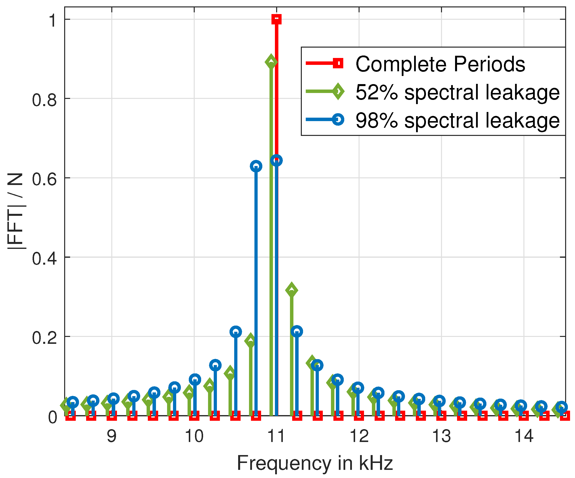
An essential property of the DFT is the discretization of the frequency vector. Assuming a large number of samples N and a sufficient resolution frequency $F_s$, the frequency resolution $f_{res}=\frac{F_s}{N}$ can provide a frequency bin $f_{bin}\left[k\right]=k·f_{res}$ that is equal or close to the desired frequency in which the AC signal analysis is desired. However, if this is not the case, a spectral leakage will occur (see Figure 1). Here both the amplitude and the frequency values split into two or more adjacent frequency bins.

Spectral leakage means that the assumed periodic signal in the time domain does not complete an exact integer period and loses its original periodicity. It can be approximated as the distance ratio to the closest frequency bin according to (4)

$$sl=2\times (0.5-|0.5-\left(t_{meas}·f-\lfloor t_{meas}·f\rfloor \right)\left|\right)$$

(4)

where $\lfloor ·\rfloor$ is the floor function and $t_{meas}$ is the total measurement time or signal duration. f is the frequency of the signal. Mathematically described, a truncated signal is a signal multiplied by a rectangular window [28], which is leaky if the periods are not complete (See Section 3.3.1). Therefore, at the frequency domain, a convolution of the results to a sinc is expected. By choosing two direct neighbor frequencies $f_{bin}\left[k\right]$ and $f_{bin}[k+1]$, with respective spectrum amplitude $y\left[k\right]$ and $y[k+1]$, the corrected frequency can be calculated via the barycenter method can be obtained using Equation (5) [28], which corresponds to the virtual non-integer frequency index q shown in (6):

$$\begin{array}{c}\hfill f_{corr}=\frac{f_{bin}\left[k\right]·y\left[k\right]+f_{bin}[k+1]·y[k+1]}{y\left[k\right]+y[k+1]}\end{array}$$

(5)

$$\begin{array}{c}\hfill q=\frac{k·y\left[k\right]+(k+1)·y[k+1]}{y\left[k\right]+y[k+1]}\end{array}$$

(6)

Therefore, the relative distance $\delta m$ between the center frequency to the nearest frequency bin is as shown in (7)

$$\delta m=q-\lfloor q\rfloor$$

(7)

The quantity $\delta m$ corresponds to $\frac{1}{2}sl$ for the frequency $f_{corr}$, as defined in (4). The corrected amplitude $A_{corr}$ and corrected phase ${\phi }_{corr}$ for the frequency $f_{corr}$ are respectively given in (8) and (9) [28]:

$$\begin{array}{c}\hfill A_{corr}=\frac{2\pi \delta m·y\left[k\right]}{sin\left(\pi \delta m\right)}\end{array}$$

(8)

$$\begin{array}{c}\hfill {\phi }_{corr}=\angle \underline{Y\left[k\right]}-\delta m\pi \end{array}$$

(9)

with $\underline{Y\left[k\right]}$ being the complex value of spectrum at bin index k. $\angle \underline{Y\left[k\right]}$ is evaluated as $\arctan 2(\Im \left(\underline{Y\left[k\right]}\right),\Re \left(\underline{Y\left[k\right]}\right))$.

2.2. Discrete-Time Fourier Transform

Discrete-Time Fourier Transform (DTFT) performs a Fourier transform on discrete-time “continuous” frequency signals [29]. Like DFT, it decomposes the signal into a sum of elementary sinewaves. Theoretically, f should be a continuous value ranging from DC to the sampling frequency $F_s$, but arbitrary frequencies are often chosen in practice. The extraction of the single-side spectrum amplitude and phase values using DTFT can be considered as a special case of finite impulse response filter, where a moving average is performed at the end of each iteration, as shown in (11) and detailed in [14].

DTFT can be explained as follows: Given a signal $x\left[k\right]=A·sin(2\pi fk\delta t+\phi )$ whose AC signal analysis, i.e., amplitude A and phase $\phi$, is desired is multiplied by 2 signals. The first is a cosine (quadrature-phase) signal with the same frequency $c=cos\left(2\pi fk\delta t\right)$, and the second is a sine signal (in-phase) $s=sin\left(2\pi fk\delta t\right)$. Alternatively, DTFT could be considered as a complex multiplication with the twiddle factor $exp\left(2i\pi fk\delta t\right)$. Averaging the output yields the real-part $\Re \left(Y\right)$ and imaginary-part $\Im \left(Y\right)$ as shown in (10) and (11), respectively:

$$\begin{array}{cc}\hfill \Im \left(Y\right)& =A\frac{cos\left(\phi \right)}{2}\hfill \\ \hfill & -\underset{\mathrm{nullified}\mathrm{when}\mathrm{N}\to \infty \mathrm{or}\mathrm{when}\mathrm{an}\mathrm{integer}\mathrm{period}\mathrm{is}\mathrm{fulfilled}}{\underbrace{A\frac{sin\left(2\pi Nf\delta t\right)}{2Nsin\left(2\pi f\delta t\right)}cos(2\pi f(N-1)\delta t+\phi )}}\hfill \end{array}$$

(10)

$$\begin{array}{cc}\hfill \Re \left(Y\right)& =A\frac{sin\left(\phi \right)}{2}\hfill \\ \hfill & +\underset{\mathrm{nullified}\mathrm{when}\mathrm{N}\to \infty \mathrm{or}\mathrm{when}\mathrm{an}\mathrm{integer}\mathrm{period}\mathrm{is}\mathrm{fulfilled}}{\underbrace{A\frac{sin\left(2\pi Nf\delta t\right)}{2Nsin\left(2\pi f\delta t\right)}sin(2\pi f(N-1)\delta t+\phi )}}\hfill \end{array}$$

(11)

Here $\delta t=1/Fs$ is the sampling period. In fact, by giving a very high number of samples, or by calculating the DTFT when the signal fulfills an integer number of periods, the real and imaginary parts will have the least influence from the spectral leakage as shown in Section 2.1.3.

2.3. Cross-Correlation (X-Corr)

Cross-correlation, abbreviated as x-corr or x-correlation, calculates the similarity between the input signal x and a reference signal y, by forming a new signal $R_{xy}$. The newly formed signal has its peak ${\Vert R_{xy}\Vert }_{\infty }=R_{xy}\left[l\right]$ at the time instance l, said to be the lag time at which maximum similarity between the two signals is observed. This time instance is the time shift between the two signals.

By using a reference sinewave signal with unitary amplitude, no initial phase, and with a frequency of choice f, the cross-correlation to a signal sharing the same frequency but a different amplitude and phases $x\left[k\right]=Asin(2\pi f\delta tk+\phi )$ returns a cross-correlation signal $R_{xy}$ signal which can be used to determine the phase and the amplitude of the signal. In this case, ${\Vert R_{xy}\Vert }_{\infty }$ at time instance l is evaluated as (12).

$$\begin{array}{ccc}\hfill R_{xy}\left[\mathit{l}\right]& =& A\frac{N}{2}cos(\phi +2\pi f\mathit{l}\delta t)\hfill \\ & -& \underset{\approx 0}{\underbrace{\frac{A}{2}\frac{sin\left(2\pi fN\delta t\right)}{sin\left(2\pi f\delta t\right)}cos(2\pi f\delta t(N-1-\mathit{l})+\phi )}}\hfill \end{array}$$

(12)

where $\delta t$ is the sampling time. Next, $R_{xy}\left[\mathit{l}\right]$ is normalized by $\frac{N}{2}$ and an integer number of periods of the signal are used to nullify the second expression. It is important to have a good phase precision when using cross-correlation to cancel $\phi +2\pi fl\delta t$. This corresponds to the existence of an integer l that verifies $-\phi \frac{Fs}{2\pi f}$. More details are given in Section 3.3. Finally, the phase can be extracted from (13).

$$\phi =2\pi \mathrm{lags}\left[\mathit{l}\right]\delta tf\left(\mathrm{mod}2\pi \right)$$

(13)

where $lags=\{-N\delta t,(-N+1)\delta t,\dots ,(N-1\left)\delta t\right\}$. Like DTFT, cross-correlation can only work with one frequency, and multi-frequency analysis requires a multiplication of the algorithm for each desired frequency.

2.4. Linear Least Squares Sine-Fit (LSQ)

Linear least squares for spectral analysis, also known as Vanicek method [12] and Sinewave-fit [13,30] uses linear regression, also known as ordinary least-squares to approximate the signal as the sum of sine and cosine signals. For a signal $x\left[k\right]=A·sin(2\pi fk\delta t+\phi )$, to which the amplitude and the phase of the frequencies $\{f_1,\dots ,f_{N_f}\}$ are desired, the linear algebra system describing the sum of sine could be written as follows:

$$A_{LSQ}p=X$$

(14)

where $A_{LSQ}$ is a $N\times 2N_f$ matrix, which contains the trigonometric coefficients, as shown in (15), X is a column vector of N elements containing the measurements and p is a column vector of $2N_f$ elements containing the linear combination coefficients of the cosine and sine signals, whose sum equals to the signal, which is analogous to the real and imaginary part of the spectrum.

$$A_{LSQ}=\left[\begin{array}{ccccc}cos\left(2\pi f_1\delta t\right)& sin\left(2\pi f_1\delta t\right)& \dots & cos\left(2\pi f_{N_f}\delta t\right)& sin\left(2\pi f_{N_f}\delta t\right)\\ cos\left(4\pi f_1\delta t\right)& sin\left(4\pi f_1\delta t\right)& \dots & cos\left(4\pi f_{N_f}\delta t\right)& sin\left(4\pi f_{N_f}\delta t\right)\\ ⋮& ⋮& ⋮& ⋮& ⋮\\ cos\left(2N\pi f_1\delta t\right)& sin\left(2N\pi f_1\delta t\right)& \dots & cos\left(2N\pi f_{N_f}\delta t\right)& sin\left(2N\pi f_{N_f}\delta t\right)\end{array}\right]$$

(15)

In this case, resolving p could be according to (16)

$$p={\left(A_{LSQ}^T{A}_{LSQ}\right)}^{-1}{A}_{LSQ}^{T}X$$

(16)

As we are using the multsine as the sum of sine, i.e., not cosines, the amplitudes and phase components of a frequency $f_k$ could be defined according to (17) and (18)

$$A_k=\sqrt{p{\left[2k\right]}^2+p{[2k+1]}^2})$$

(17)

$$A_k=atan2(p\left[2k\right],p[2k+1]))$$

(18)

2.5. Non-Linear Least Squares Sinewave Fitting (NLSQ)

Linear and non-linear least-squares curve fitting algorithms have been used for AC signal analysis to reduce random noise and eliminate the effects of systematic distortions that could affect the amplitude and phase spectrum, as depicted in [31]. A major difference from the previous paragraph is the use of a non-linear model for the sinewave fitting. Here the model is assumed as the sum of $N_f$ sinewaves, with amplitudes $A_k$ and phases ${\phi }_k$ as shown in (19)

$$x_{fit}\left[n\right]=\sum _{k=1}^{N_f}{A}_{k}sin(2\pi f_{k}n·\delta t+{\phi }_k)$$

(19)

By setting a variable vector $\beta$ at iteration (i), ${\beta }_{\left(i\right)}=\left[\begin{array}{cccccc}{A}_1& \dots & A_{N_f}& {\phi }_1& \dots & {\phi }_{N_f}\end{array}\right]$, (19) becomes (20)

$$x_{\left(i\right),fit}\left[n\right]=\sum _{k=1}^{N_f}{\beta }_{\left(i\right)}\left[k\right]sin(2\pi f_{k}n·\delta t+{\beta }_{\left(i\right)}[k+N_f])$$

(20)

By iterating (21) several times until a maximum number of iterations MAX_ITER is reached, or until a convergence criterion (25) is achieved, the final value of ${\beta }_{\left(i\right)}$ stores the values of the amplitudes and phases.

$${\beta }_{\left(i\right)}={\beta }_{(i-1)}+{\left(J_{\left(i\right|i-1)}^T{J}_{\left(i\right|i-1)}\right)}^{-1}{J}_{\left(i\right|i-1)}^T{r}_{\left(i\right)}$$

(21)

with $J\left(i\right|i-1)$ is the Jacobian Matrix in iteration (i) which takes the following form (22):

$$J_{\left(i\right|i-1)}=\left[\begin{array}{cccccc}\frac{\partial r_{\left(i\right)}\left[1\right]}{\partial A_1}& \dots & \frac{\partial r_{\left(i\right)}\left[1\right]}{\partial A_{N_f}}& \frac{\partial r_{\left(i\right)}\left[1\right]}{\partial {\phi }_1}& \dots & \frac{\partial r_{\left(i\right)}\left[1\right]}{\partial {\phi }_{N_f}}\\ ⋮& & ⋮& ⋮& & ⋮\\ \frac{\partial r_{\left(i\right)}\left[N\right]}{\partial A_1}& \dots & \frac{\partial r_{\left(i\right)}\left[N\right]}{\partial A_{N_f}}& \frac{\partial r_{\left(i\right)}\left[N\right]}{\partial {\phi }_1}& \dots & \frac{\partial r_{\left(i\right)}\left[N\right]}{\partial {\phi }_{N_f}}\end{array}\right]$$

(22)

and $r_{\left(i\right)}\left[n\right]=x_{\left(i\right)}\left[n\right]-x_{\left(i\right),fit}\left[n\right]$ is the residual at time instance n to the actual data, at iteration (i). Their partial derivative at time n with respect to the amplitude $A_k$ and phase ${\phi }_k$ are depicted in Equations (23) and (24), respectively.

$$\begin{array}{ccc}\hfill \frac{\partial r_{\left(i\right)}\left[n\right]}{\partial A_k}& =& -sin(2\pi f_{k}n\delta t+{\phi }_k)\hfill \\ & =& -sin(2\pi f_{k}n\delta t+{\beta }_{(i-1)}[N_f+k])\hfill \end{array}$$

(23)

$$\begin{array}{ccc}\hfill \frac{\partial r_{\left(i\right)}\left[n\right]}{\partial {\phi }_k}& =& -A_{k}cos(2\pi f_{k}n\delta t+{\phi }_k)\hfill \\ & =& -{\beta }_{(i-1)}\left[k\right]cos(2\pi f_{k}n\delta t+{\beta }_{(i-1)}[N_f+k]))\hfill \end{array}$$

(24)

The algorithm would achieve either a maximum number of iterations MAX_ITER or the convergence criterion shown in (25):

$$\Vert {\beta }_{(i-1)}-{\beta }_{\left(i\right)}\Vert <\epsilon$$

(25)

3. Comparison among Different AC Signal Analysis Methods

3.1. Processing Time

Analysis time or processing time is a particularly principal factor that determines the speed of AC signal analysis. However, with today’s progress, the comparison of the algorithms has become very practical and hardware/software-specific as hardware acceleration chips are being integrated into both generic computers and embedded systems to speed up analysis.

Among existing hardware accelerations are data-level parallelism, such as Single-Instruction Multiple-Data, where a large amount of data is processed simultaneously. Alternatively, instructions are parallelized, to execute concurrently or interleaved depending on the microprocessor’s architecture; For a single-core microprocessor, the instructions are executed interleaved to assure finishing the tasks at the same time. For multi-core multiprocessors, the instructions are split into different cores and are executed in parallel.

These accelerations are typically determined by a combination of program code which should target these hardware optimizations, compiler settings, and hardware capabilities. In this section and as a first step, we focus on the theoretical processing time of each AC signal analysis for generic computing without hardware acceleration. Then, in the second part, we discuss the possible hardware acceleration for each AC method in detail.

3.1.1. Theoretical Algorithm Complexity

In this section, we define the complexity of the algorithm according to two factors: N is the number of samples to be processed and $N_f$ is the number of frequency components whose associated amplitudes and phases are desired. This complexity gives information about the expected asymptotic time response per number of samples and the double of the number of frequency components (Double, due to amplitude and phase, or real and imaginary part determination).

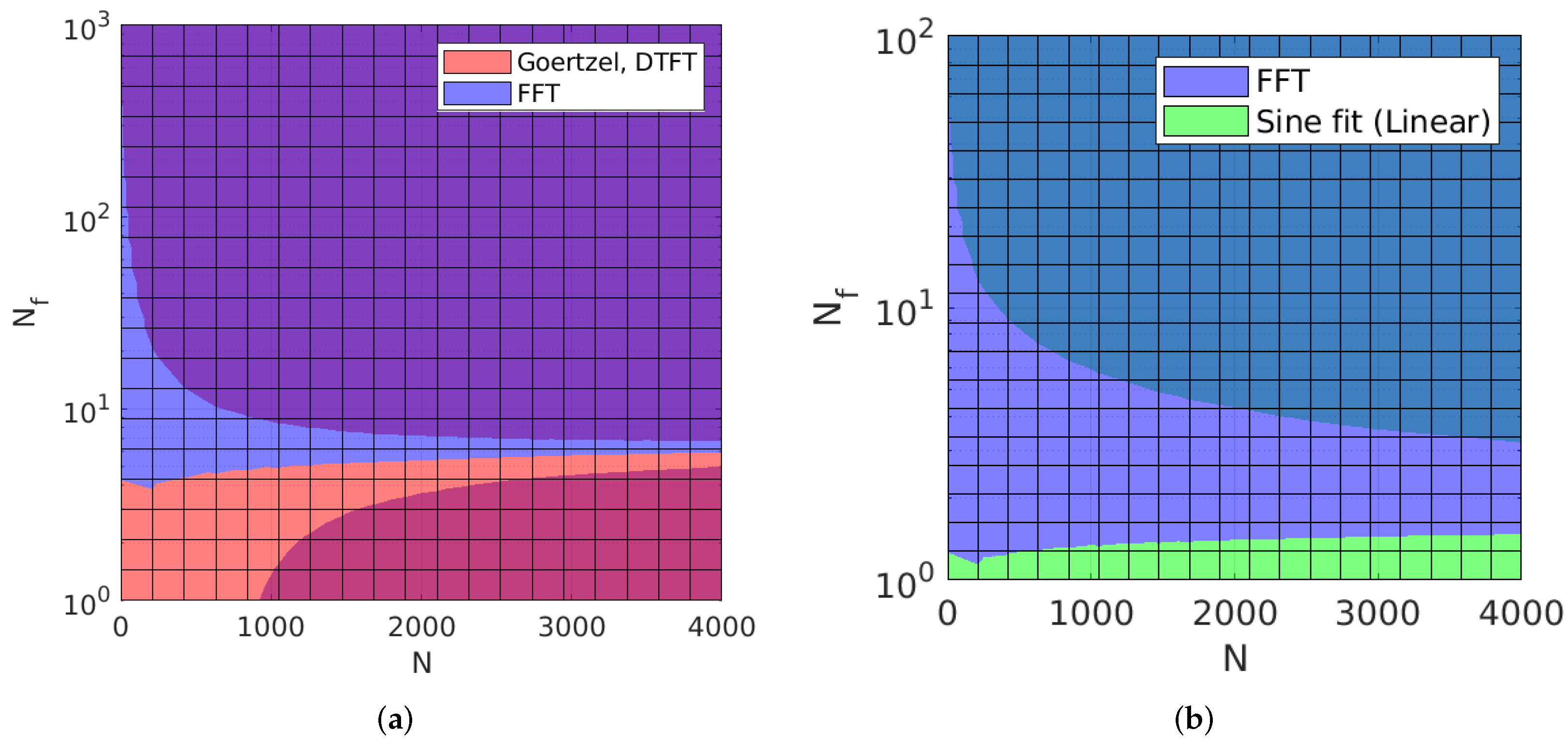
All algorithms are described in

Table 1. Comparison between Computation Complexity of Several Methods of AC signal analysis per Number of Samples and Number of Frequency Components.

Method	Type	Comp. Complexity	n. op/Iteration
FFT (Radix-2/4/8)	Transform	$O(\mathrm{N}{\log }_2\mathrm{N})$	-
Goertzel	Filter	$O\left(2\mathrm{N}{N}_f\right)$	6 $N_f$
Cross-Correlation	Transform	$O\left(2N_f{N}^2\right)$	-
Sine-fit (linear)	Transform	$O\left(({\left(2N_f\right)}^3+{\left(2N_f\right)}^{2}N+2N_{f}N)\right)$	-
Sine-fit (non-linear)	Transform	$O\left(n_{iter}({\left(2N_f\right)}^3+{\left(2N_f\right)}^{2}N+2N_{f}N+N)\right)$	-
DTFT	Filter/Transform	$O\left(2N{N}_f\right)$	6$N_f$ or 14 $N_f$

. Theoretically, DTFT and Goertzel would have similar times as they both have the least complexity among the algorithms compared. Most of the computation consists of multiplication and accumulation, operating on the desired frequencies only, which makes them linear to both N and $2N_f$. For a small number of frequencies $N_f$, they may outperform FFT (Radix-2, or Radix-4, or Radix-8). However, from an approximate of $N_f>lo{g}_2\left(N\right)$, FFT provides similar or lower computation times. In Figure 2a, the visualization of the better algorithm as a function of time complexity is shown. In this graph, the boundary line $N_f>lo{g}_2\left(N\right)$ separates the two regions where Goertzel/DTFT are expected to have slightly lower complexity (red shades colors) and the regions where FFT has lower complexity (purple shades). Clear red and purple define ambiguous regions, in which one may out perform the other. Finally, DTFT and Goertzel’s performances are not the same: While Goertzel uses a constant twiddle, requiring $6N_f$ operation per iteration, DTFT requires the twiddle to be calculated for each point. Therefore, a coefficient lookup table for DTFT may be required to obtain $6N_f$ operations per iteration, otherwise, $14N_f$ operations per iteration are required. In addition, if $2\pi$ is not set as a constant, or if time information, i.e., $n\delta t$, is not calculated beforehand, an additional $2N_f+2N_f$ operation for DTFT per iteration should be included.

Cross-correlation is done by the multiplication and addition of the reference signal that is shifted in time to the input signals, requires for all the samples. It, therefore, has a complexity of $O\left(2N^2{N}_f\right)$. Next are the sine-fit methods. For linear least-squares sine-fit, the multiplication of $A_{m}at$ to its conjugate has a time complexity of $O\left({\left(2N_f\right)}^{2}N\right)$. The inversion can be done using cofactor or adjoint matrix, one taking $O((2N_f+1)!)$ while the other $O\left({\left(2Nf\right)}^3\right)$, assuming adjoint method is used for inversion as it provides better performance for small $N_f$, a complexity $O\left({\left(2Nf\right)}^3\right)$ is required for matrix inversion. Last are two multiplications with respective complexity of $O\left({\left(2N_f\right)}^{2}N\right)$ and $O\left(2N_{f}N\right)$. Therefore, the overall complexity could be estimated to $O({\left(2N_f\right)}^{2}N+{\left(2N_f\right)}^3+2N_{f}N)$. Compared to FFT and shown in Figure 2b, the time complexity of linear least-squares sine-fit is less than FFT if there is only one frequency component. Otherwise, FFT has a slight advantage for $N_f<100$, as indicated by light bluish-purple in the graph. On the other hand, the turquoise region shows a clear advantage of FFT over the linear least-squares in terms of time complexity, when $N_f>100$.

Next is the non-linear least square sine fitting, which has similar requirements as linear least-squares, since it is based on linearization process through gradient operator, in addition to multiple iterations $n_{iter}$ needed to achieve the goal. In addition, the signal reconstruction requires $N{N}_f$ iterations, and an additional N subtraction operations are also required for the calculation of the parameters. Summing together, the overall time asymptotic complexity of non-linear sine-fit is $O\left([{\left(2N_f\right)}^{2}N+{\left(2N_f\right)}^3+2N_{f}N+N]n_{iter}\right)$.

3.1.2. Possible Hardware Acceleration

Although hardware acceleration is possible for all AC signal analysis methods, only some hardware acceleration methods could be relevant due to the computational overhead required before parallelization, such as filling arrays, etc. Other methods require more time to set up the context per each thread or transfer data to the dedicated units, negating the efficiency of the parallelism.

In

Table 2. Efficient Hardware Acceleration Methods for AC signal analysis Methods Treated in this paper.

Method	Possible Parallelism Method
	Data-Level	Instruction-Level
FFT (Radix-2/4/8)	x	x
Goertzel	x	x
Cross-Correlation	x	x
Sine-fit	x
DTFT	x	x

, we summarize the optimal acceleration methods for the AC signal analysis, whether data-level or instruction-level parallelism is relevant to the considered method.

First, and for FFT (Radix-2, or Radix-4, or Radix-8), block calculation can be accelerated by either using data-level or instruction-level parallelism or both. Data-level parallelization provides a more efficient way to compute the twiddle coefficients. It can also be used to evaluate the expressions within each radix block calculation or by concatenating them into a single vector. Alternatively, each radix block can be evaluated within one thread. Second, Both of Goertzel filter and DTFT computation can be parallelized at either data or instruction level to parallelize the calculation of each frequency component. When possible, concatenating all calculations in single or multiple vectors allows for more efficient parallelization. Third, Cross-correlation computation can be accelerated at the data level by concatenating all computation in a single vector or multiple vectors. Alternatively, parallelization can be performed at the instruction level for each frequency component. Fourth, Sine fitting can exploit data-level parallelism to calculate the novel signal. However, due to the sequence of its steps, parallelizing instructions is not efficient.

3.2. Memory Usage

This paragraph discusses the memory allocation required by each algorithm. The results reflect the expected approximate memory allocation within a generic floating-point-enabled processor, including stack memory usage.

Table 3. Comparison between the Memory Allocation Excluding Signal Length Required for the AC signal analysis.

Method	Required Memory Cases
FFT	N or 2N, plus additional 14–50 cases
Goertzel	7$N_f$
Cross-Correlation	$N_f$·(N+2) + 3, plus either 1 or $N{N}_f$
	SIMD: (2N+2)·$N_f$ + 3 + optional $2N$ + $3N$
Sine-fit (linear)	6$N{N}_f$ + 8 $N_f^2$ + 2 $N_f$
	• Cofactor/Adjoint, determinant, transpose require up to $4N_f^2+8$ cases
Sine-fit (non-linear)	6$N{N}_f$ + 2 N + 8 $N_f^2$ + 2 $N_f$ + 2
	• SIMD requires N for intermediate calculations
	• Cofactor/Adjoint, determinant, transpose require up to $4N_f^2+8$ cases
DTFT	$4N_f$, plus either 2 or $2N{N}_f$

shows an overview of the memory required by each algorithm without the input signal. Here N defines the number of samples and $N_f$ the number of frequency components. The uncertainty comes from the values from the practical Visual C++ and STM32CubeIDE application.

FFT can be performed in-place or out-of-place. In the case of in-place FFT, a complex format of the signal on which the FFT is performed is required and therefore additional N cases is required, as signals mostly real. For the out-of-place FFT algorithms, $2N$ cases are necessary to compute the values of the single-sided spectrum analysis. During the calculation in the in-place or out-of-place implementation, several cases are required for storing intermediate results, DFT twiddles/coefficients, and for bit reversing. Those cases may be around 14 to 50 cases depending on the chosen radix and the implementation method. The Goertzel filter requires 3 cases per frequency component to store the results, in addition to 2 more cases per frequency component for the coefficients, which could be replaced by 2 local memory cases. At the end of the processing, 2 more cases are needed to calculate the DFT values per frequency component.

The memory requirement of cross-correlation is dependent on the reference signal and the output size. If half of the output is desired and the reference signal is the same length as the input signal, the total required memory to store the results is $N{N}_f$. To store the position of the absolute value as well as its index, at least 2 additional cases per frequency component are necessary. For each frequency component, an additional memory case or a lookup table of N is needed. For the loop iterators, 3 more cases are needed. Typically, Standard and SIMD Cross-correlation require $2N$ to store the data, in addition to optional $2N$ cases to calculate absolute values. The largest absolute value and its index require $2N_f$ cases. 3N buffer cases may be required to store intermediate results needed to construct the reference signal per each frequency component and to square the signal to prepare for energy calculation. The latter also requires one more case for the sum. Iterators require two further cases.

Sine fitting requires the assignment of many matrices during the calculation. For linear least-squares sine fitting, 2 matrices $2N_f\times N$, 1 matrix $N\times 2N_f$ and 2 matrices $2N_f\times 2N_f$ are required, in addition of the variable vector $2N_f$. For the matrix inversion, $4N_f^2+8$ more cases are required. The non-linear sine-fit adds to the requirements needed in sine-fitting a vector containing the currently estimated signal with N elements, and the residual vector $2N_f$. 2 N intermediate memory cases may be required to store signal after each iteration. At least 2 more cases for loop iterators are needed in addition.

DTFT requires 2 memory cases per frequency component to store the result. A $2N{N}_f$ lookup table is required for the DTFT coefficients, which could be replaced by 2 local memory cases. Eventually, 2 more cases are required to calculate the final single-sided spectrum amplitude values.

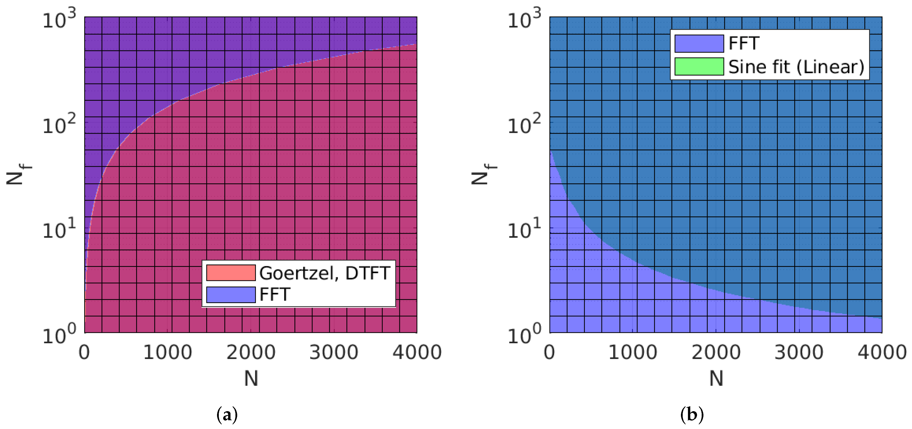
When these results are visualized, it is shown that Goertzel, then DTFT is advantageous in most of the cases, as compared to FFT as shown in Figure 3a. Although, on the other hand, FFT requires less memory than sine fitting (linear/non-linear) and cross-correlation, the asymptotic memory usage of Sine-fit linear, non-linear, and cross-correlation is similar. Therefore only one example (Sine-fit) was visualized in Figure 3b in comparison to FFT. In this graph, the FFT has a slight advantage in the light purple area and a landslide advantage in the turquoise area.

3.3. Influence of Spectral Leakage on the Accuracy of the Amplitude and Phase

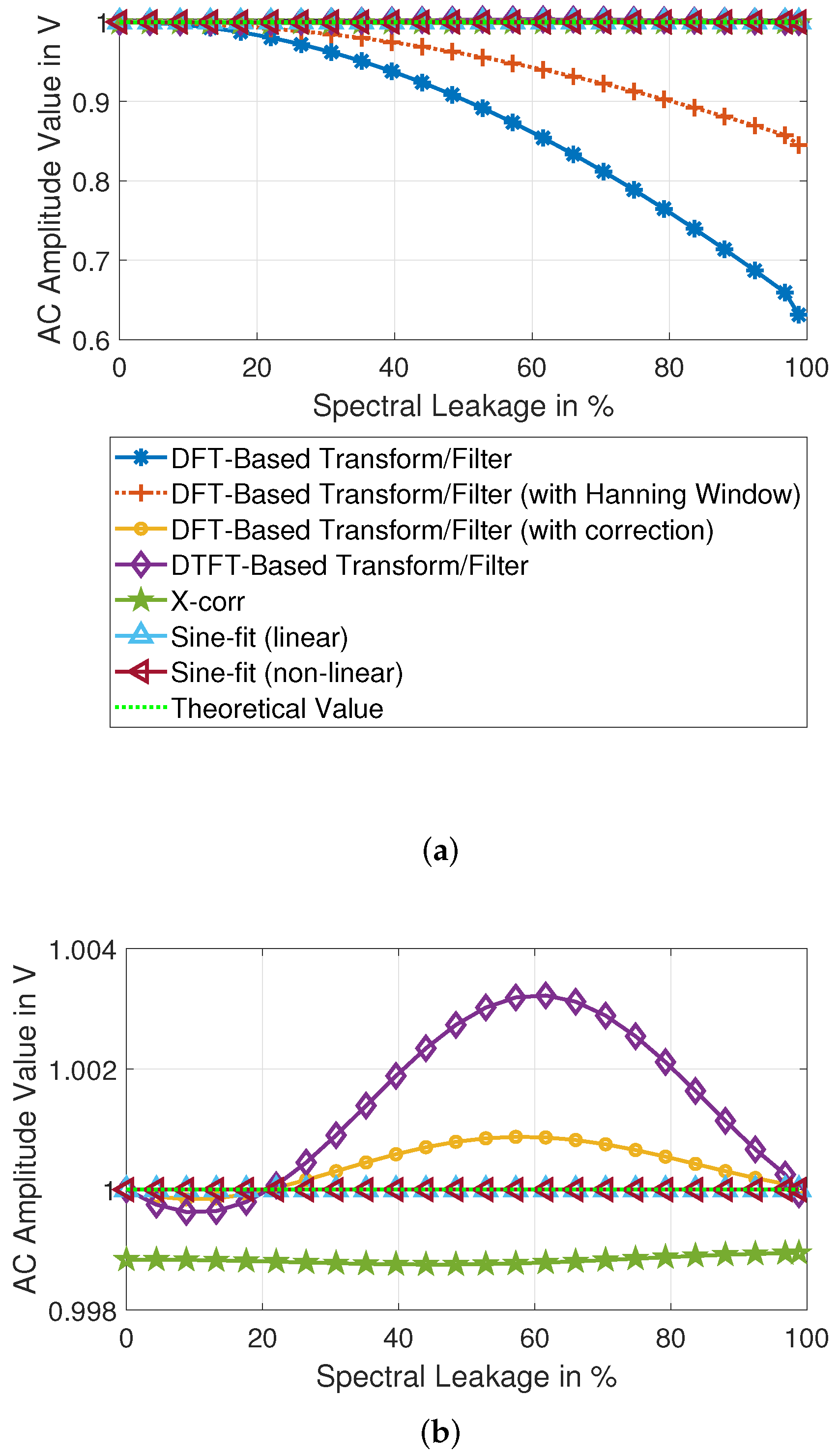
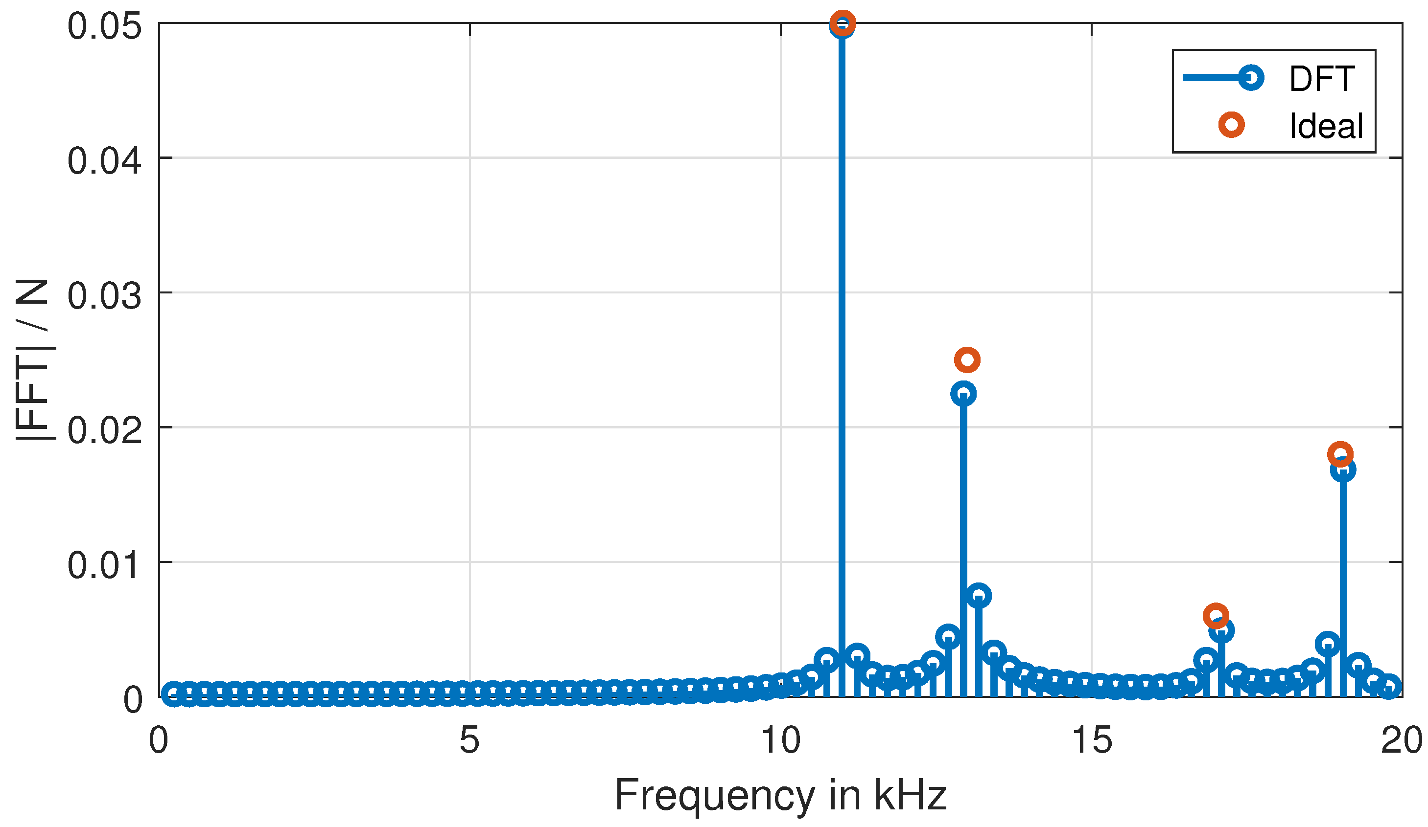
In this section, we also consider the general sinewave response signal $x\left[k\right]=A·sin(2\pi ft+\phi )$ with a length of N as an example for the theoretical part. An exemplary signal of 11 kHz with amplitude $A=1V$ and phase $\phi =\frac{\pi }{6}$, sampled at a rate of $F_s$ = 500 kHz, is used as a test scenario. The number of samples is 2048, the spectral leakage is 11.2%, and the distance to the nearest frequency bin $k=45$, corresponding to $f_{bin}\left[45\right]$ = 10,986.328 Hz, is $\delta m=0.05$. In the first part, we study the accuracy and precision of the amplitude values, while in the second part, we consider the accuracy and precision of the phase values. We note that DFT in this section represents both FFT and Goertzel.

3.3.1. Amplitude AC Signal Analysis Accuracy

Theoretically, all the AC signal analysis methods project the signals into an orthogonal Fourier basis formed by trigonometric reference signals, hence, no signal interference is expected, if the signal is a multisine. In practice, the signals are finite, hence, truncated. In the point-of-view of Fourier analysis, this truncation is none other than multiplication with a rectangular window in the time-domain and a convolution by sinc in the frequency domain. For incomplete signals, not only the desired frequency but also nearby frequencies are influenced. For example, for DTFT, the extra coefficients (10) and (11) become remarkable and are not nullified. The same problem is also spotted in DFT; Considering a distance to the closest frequency bin $\delta m$, its amplitude deviation is, therefore, $A(1-sinc(\delta m\left)\right)$. The use of window function, such as Hanning window function [32], for example, minimizes, but does not eliminate, the deviation to $A(1-\frac{sinc\left(\delta m\right)}{1-\delta m^2})$[28]. Similarly for DTFT, the deviation formula is demonstrated in Appendix A and depicted in (26) where $R=\frac{sin\left(2\pi fNdt\right)}{sin\left(2\pi fdt\right)}$.

$$\overline{\Vert X_{DTFT}\Vert }=A\left(1-\sqrt{1+{\left(\frac{R}{N}\right)}^2-2\frac{R}{N}cos(2\phi +2\pi f(N-1)\delta t)}\right)$$

(26)

However, this expression is not predictable when the initial phase is unknown. Therefore, assuming the worst case, it can be simplified to (27)

$$\overline{\Vert X_{DTFT,simp·}\Vert }=A\frac{sin\left(2\pi fN\delta t\right)}{Nsin\left(2\pi fdt\right)}\approx A\frac{sin\left(2\pi \delta m\right)}{Nsin\left(2\pi fdt\right)}$$

(27)

Since the FFT correction based on Section 2.1.3 generates a new frequency that emulates the DTFT, its behavior could be modeled as in (26), but with a different R-expression, since it inherits the behavior of the rectangular window from the original FFT. R then becomes $R=\frac{sinc\left(\delta m\right)sin\left(2\pi fNdt\right)}{sin\left(2\pi fdt\right)}$. The expression of the simplified corrected FFT for the worst case is then $A\frac{sinc\left(\delta m\right)sin\left(2\pi \delta m\right)}{Nsin\left(2\pi fdt\right)}$.

Cross-correlation loses its accuracy if the amplitudes from the AC signal analysis are very different due to the use of $L_{\infty }$ norm for amplitude and phase determination. In addition, it is also affected by the signal incompleteness, as shown in (12), as well as the resolution of the $\phi$ phase. To obtain accurate results, two conditions must be met: For the frequency in question, an integer number of periods; and an adequate phase resolution are required to satisfy the existence of an integer time l that satisfies $l=-\phi \frac{F_s}{2\pi f}$. This means that $\frac{F_s}{f}$ should be as low as possible. The maximum amplitude deviation expression, given a good phase resolution, could be simplified to the same expression as for DTFT (27), albeit with a negative sign.

Finally, sine-fitting methods show little to no sensitivity to spectral leakage due to both of them being solutions to inverse algebra problems.

For the exemplary signal and as shown in Figure 4b and summarized in

Table 4. Comparison between the sensitivity of the amplitude AC signal analysis methods to interference and to spectral leakage.

2pt Method	Sensitivity to Interference	Sensitivity to Spectral Leakage	Approx. Max. amp. Deviation Formula.	Max Deviation (Application/Figure 4a)
DFT-based	Low	Very High	$A(1-sinc(\delta m\left)\right)$	36%
DFT-based and windowed (Hann)	Low	High	$A(1-\frac{sinc(\delta m}{1-\delta m^2})$	15%
DFT-based and corrected	Low	Very Low	$\frac{Asinc\left(\delta m\right)}{N}\frac{sin\left(2\pi \delta m\right)}{sin\left(2\pi f\delta t\right)}$	0.08%
DTFT	Low	Low	$\frac{A}{N}\frac{sin\left(2\pi \delta m\right)}{sin\left(2\pi f\delta t\right)}$	0.32%
X-corr	High	Low	−$\frac{A}{N}\frac{sin\left(2\pi \delta m\right)}{sin\left(2\pi f\delta t\right)}$	0.27%
Sine-fitting	Low	Insensitive	-	0%

, the sine-fitting methods show no uncertainty. The second best is DFT with correction with a maximum deviation of 0.08%, then cross-correlation with a maximum deviation of 0.27%, then DTFT with a maximum deviation of 0.32%. Although the windowing allowed a lower maximum deviation of 15%, it is still considered high. The strongest influence is seen with the DFT algorithm without correction, with a maximum deviation of 36%.

3.3.2. Phase AC Signal Analysis

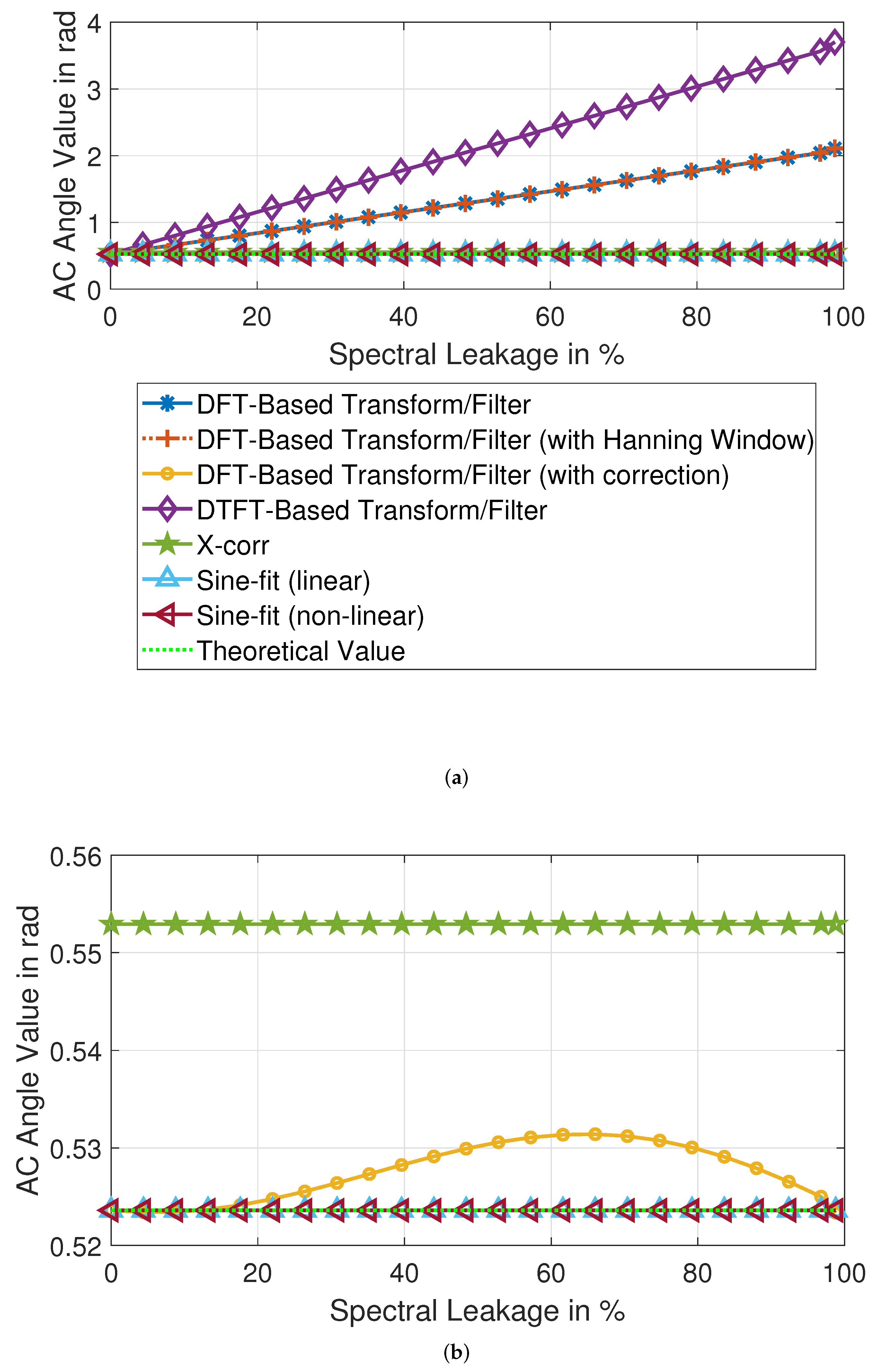
Spectral leakage affects the signal’s shape in the frequency domain, which eventually affects the phases for DFT and DTFT-based methods unless a correction formula is present for Fourier-based methods. On the other hand, the phase in the cross-correlation is mainly affected by the $L_{\infty }$ norm in addition to the phase resolution, which is $\frac{2\pi f}{F_s}$. Among all the solutions, only sine fitting solutions have the least influence by the spectral leakage during phase determination.

Analytically, the deviation expression can be intuitive, such as in the case of DFT and sine-fitting, but can also be convoluted in the other methods due to the non-linear behavior of the arc tangent of imaginary and real parts used in the phase calculation. In these cases, it is necessary to calculate the deviation in Cartesian coordinates beforehand. In DFT, with or without windowing, the phase deviation is always $\delta m\pi$. The phase analysis using cross-correlation depends mainly on the phase resolution. Sine-fitting methods show lower sensitivity to phase uncertainty. However, for DTFT and DFT with correction, the Cartesian calculation is necessary to derive the phase uncertainty. For this purpose, numerical simulations and test scenario studies are preferably used.

Table 5. Comparison between the sensitivity of the phase AC signal analysis methods to interference and to spectral leakage.

3.5pt Method	Sensitivity to Interference	Sensitivity to Spectral Leakage	Max Deviation (Application/Figure 4a)
DFT-based	Low	Very High	$\raisebox{1ex}{$\pi $}\!\left/ \!\raisebox{-1ex}{$2$}\right.$ rad
DFT-based and windowed (Hann)	Low	Very High	$\raisebox{1ex}{$\pi $}\!\left/ \!\raisebox{-1ex}{$2$}\right.$ rad
DFT-based and corrected	Low	Low	0.0078 rad
DTFT	Low	Low	0.0029 rad
X-corr	High	Low	0.0293 rad
Sine-fitting	Low	Insensitive	$1.44\times {10}^{-15}$ rad

summarizes these deviations.

When applied to the example signal for phase spectroscopy, it can be seen that sine fitting methods give the most accurate results. The maximum deviation is in the range of ${10}^{-15}$ resp. ${10}^{-14}$. DTFT has the third-lowest maximum deviation of 0.0293 rad, followed by DFT with correction, with 0.0078 rad. While the cross-correlation is not affected by the spectral leakage, as shown in Figure 5a, the phase resolution defines its precision, and therefore the constant deviation, independent of the spectral leakage, is 0.0293 rad. Finally, both the DFT with and without windowing yielded a maximum deviation of $\frac{\pi }{2}$, as shown in Figure 5a. A summary of the methods is shown in Table 5. The values of the phases are plotted against spectral leakage in Figure 5a, with a closer look in Figure 5b.

4. Test Scenario: AC Signal Analysis of the Sum of 4 Sines with Arbitrary Frequencies

In this section, we apply the previously mentioned algorithms for AC signal analysis to a multisine signal consisting of the sum of 4 sinewaves with arbitrary amplitudes and phases based on matrix measurements of [33]. The sampling frequency is set to 500 kHz. The properties of the signals are shown in

Table 6. Chosen Signal Properties as a Test Scenario.

Frequency (kHz)	Amplitude (V)	Phase (rad)	sp. lk (%)
11	0.05	0	11.2%
13	0.025	$\raisebox{1ex}{$\pi $}\!\left/ \!\raisebox{-1ex}{$4$}\right.$	49.6%
17	0.006	$\raisebox{1ex}{$\pi $}\!\left/ \!\raisebox{-1ex}{$6$}\right.$	73.6%
19	0.018	$\raisebox{1ex}{$\pi $}\!\left/ \!\raisebox{-1ex}{$2$}\right.$	35.2%

. The number of samples is set to a constant 2048.

The analysis follows in five different setups. The first platform is a reference to provide information on the performance of the methods on a generic computer. It consists of a generic Windows personal computer with a CPU Intel Core (TM) i7-7700HQ @ 2.80 GHz and 16 GB RAM. The CPU supports several SIMD instructions, including SSE2 and AVX instructions, which provide hardware acceleration to MATLAB code thanks to Intel Math Kernel Library (MKL) and FFTW-3.3.3-SSE2-AVX library. For a second reference, the codes are reimplemented in C using Visual C++, which uses a compiler optimization for the hardware.

The second platform is the STM32-based evaluation board STM32H743Zi. It features an Arm Cortex-M7 CPU clocked at 480 MHz, which is coupled with 1MB RAM. The built-in ADC is capable of a sampling rate of at 4 MSps, with at least sub GHz-bandwidth [34]. In this platform, two environments are used: The first one features the computation of algorithms with double-precision floating points. The methods are written in C and compiled in MCU GCC Compiler with no further optimization or hardware acceleration aside from compiler’s. In a second environment, Cortex Microcontroller Software Interface Standard (CMSIS) instructions were used to speed up the computation. The CMSIS-DSP library for Cortex-M7 for single-precision floating points calculations was used to calculate SIMD instructions when possible. The third platform is Teensy 3.6, which is programmed using Teensyduino, a software package for Arduino IDE. It features a Cortex-M4 CPU clocked at 180 MHz and 256 kB RAM. The built-in ADC is capable of a sampling rate of sub-MHz range, with a bandwidth of sub-GHz range. It is worth noting that for both microcontrollers and according to the Nyquist criteria, the maximum frequency should be less than half the sampling rate.

All the decimals are stored and processed as double-precision floating points unless otherwise noted. As CMSIS-DSP only supports single-precision floating-point, the decimals are implemented with single-precision floating-point. In most cases in native STM32 C code, we found that the native double-based trigonometric functions are faster than single float-based trigonometric functions. Further implementation details are discussed in this section.

The FFT is implemented using the FFTW library in MATLAB 2021a, Radix-2 in Visual C++, and STM32/Teensy Native code, and using a mixed-radix based on Radix-8 on CMSIS-DSP implementation. Cross-correlation was implemented with a lookup table (LUT) in all the implementations. Moreover, cross-correlation without LUT was proven to be more efficient only in STM32 native C, as explained in the next sections. The curve fitting was implemented with double precision in generic computing and both single and double precision in STM32 native C. In CMSIS-DSP, only the supported single-precision floating-point was used. DTFT was implemented with a LUT in generic computing and CMSIS-DSP and both with and without it in Native C.

Finally, MATLAB and CMSIS-DSP data are always vectorized, i.e., with lookup tables whenever possible, to enable hardware acceleration through SIMD instructions. In STM32 native C code, the trigonometric functions from the math library were used, while in the DSP-CMSIS library, the Arm-exclusive trigonometric functions were used instead. The methods were run multiple times. A total memory clear and removal of memory cache was ensured between runs by restarting the program/device several times.

4.1. Processing Time

In Section 3.1, the asymptotic complexity and the expected runtime as a function of the number of samples and frequency components were presented. However, as mentioned before, the actual processing time may differ due to the different optimization on the hardware/software side.

According to Section 3.1, the proposed scenario falls in the ambiguous region where Goertzel, DTFT, and FFT should have similar asymptotic computations, with an advantage for Goertzel and DTFT. They are then followed by linear sine-fit, nonlinear sine-fit, and cross-correlation ranked according to their ascending computational complexity. Nevertheless, it is important to consider the number of iterations, including overhead operations before or during the calculation process. This includes the computation of look-up tables, twiddle factors, and the computation of in-place coefficients for each algorithm. In fact, DTFT actually requires $14N_f$ up to $18N_f$ per iteration, while FFT Radix 2 only requires $5lo{g}_{2}N$. Therefore, for this test scenario, $55N$ operations are required for the FFT and $56N$–$72N$ operations for the DTFT. The Goertzel filter requires only $6N_f$ operations per iteration, resulting in $24N$ total operations, which should make it the fastest algorithm for this test scenario.

As shown in

Table 7. Total AC signal analysis Processing Time as Implemented in MATLAB and Visual C++ in ms.

-	MATLAB	PC/C (Visual C++)
FFT	0.51	0.81
Goertzel	7.92	0.51
X-corr	76.64	377.95
Sine-fit (linear)	8.02	2.10
Sine-fit (non-linear)	91.08	70.39
DTFT	10.98	0.92

, MATLAB results show that FFT is the fastest owing to the optimized FFTW3 library with a total processing time of 0.51 ms, followed by Goertzel (7.92 ms), then sine-fit linear (8.02 ms), then DTFT (10.98 ms), then cross-correlation (76.64 ms), and finally sine-fit (non-linear) (91.08 ms).

On the other hand, the results of Visual C++ match the expected theoretical results, as Goertzel filter is the fastest with 0.51 ms processing time, followed by FFT (0.81 ms), then DTFT (0.92 ms), then Sine-fit (2.1 ms), then sine-fit non-linear (70.39 ms), and finally cross-correlation (377.95 ms).

Table 8. Total AC signal analysis Processing Time as Implemented in Non-accelerated and Hardware-accelerated Environment in STM32 and Teensyduino 3.6.

	STM32	Teensy 3.6	STM32
	(Native/Double)	(Teensyduino/Double)	(CMSIS/Float)
FFT	99 ms	76 ms	8 ms
Goertzel	21 ms	57 ms	18 ms
	$\tilde{}$ 10 μs per iter.	$\tilde{}$ 27 μs per iter.	$\tilde{}$ 8 μs per iter.
X-corr	67 s	82 s	4 s
Sine-fit (linear)	638 ms	296 ms	139 ms
Sine-fit (non-linear)	58 s	38 s	12 s
DTFT	132 ms	280 ms	28 ms
	$\tilde{}$ 64 μs per iter.	$\tilde{}$ 136 μs per iter.	$\tilde{}$ 13 μs per iter.

shows the comparison between the native double-precision code implementation of the algorithm in STM32, native code implementation in Teensy, and STM32 optimized using CMSIS DSP library. In STM32 native implementation, Goertzel is the fastest algorithm with 21 ms runtime, followed by FFT with 99 ms, then DTFT with 132 ms, then sine-fit (linear) with 638 ms, then sine-fit (non-linear) with 58 s, and finally cross-correlation with 67 s. The same rank is seen for Teensy 3.6 implementation. However, this rank changes when the methods are implemented using CMSIS-DSP on STM32: FFT is the fastest with 8 ms runtime, followed by Goertzel with 18 ms, then DTFT with 28 ms, then sine-fit (linear) with 139 ms, then cross-correlation with 4 s, and finally sine-fit (non-linear) with 12 s.

At this point, it can be stated that the influence of hardware and software should not be underestimated. However, for native PC (Visual C++) and embedded implementations, the rank of each method is the same on each platform, which is consistent with the theoretical values in Figure 6. For the hardware-accelerated CMSIS implementation, the mixed radix implementation together with hardware acceleration was able to push DTFT behind FFT. Finally, during the experimentation, we noticed that all algorithms showed a slowdown when implemented with single-precision float functions, i.e., cosf and sinf, and that the CMSIS DSP library provides the fastest solutions for trigonometric operations.

As a partial conclusion: For this or a similar scenario, when the number of frequencies is small and when using a hardware-accelerated calculation, FFT is the fastest option for AC signal analysis. Second to FFT is the Goertzel filter, which is relatively fast in both hardware-accelerated generic and embedded computing systems and is slightly faster than DTFT. In a native implementation scenario, i.e., with no to less hardware acceleration, Goertzel performs the fastest, which is confirmed in both PC (Visual C++) and STM32/Teensyduino implementations. While DTFT’s trigonometric solution is accelerated in PCs, its embedded implementation counterpart lags behind. For this reason, DTFT is considered less efficient than FFT for embedded systems with the same or similar specifications for this test scenario.

4.2. Memory Usage

In this section, we compare the memory usage required for the designed scenario. Goertzel and DTFT (without LUT) have the lowest memory consumption, as given in

Table 9. Comparison of the memory consumption of the AC signal analysis methods in the native C and vectorized hardware-accelerated implementation.

Method	Req. Cases	Actual Memory Use in kB
		Native Embedded/Double	STM32 Using CMSIS-DSP/Float
FFT	2062–4146	32.09 kB (4110 cases)	8.14 kB (2086 cases)
Goertzel	28	224 bytes	112 bytes
X-corr (without LUT)	8204	64.05 kB	-
X-corr (with LUT)	26,633	-	74.01 kB
Sine-fitting (linear)	49,936	390.12 kB	195.06 kB
Sine-fitting (non-linear, float)	≈55,450	208.81 kB (55,457 c.)	216.56 kB (55,441 c.)
Sine-fitting (non-linear, double)	≈55,450	417.14 kB (55,457 c.)	-
DTFT (without LUT)	18	132 bytes	-
DTFT (with LUT)	16,402	128.13 kB	64.06 kB

. Sorted from highest to lowest memory requirements, non-linear least squares sine-fit requires the highest memory allocation, with around 55 k cases, then linear least-squares sine-fit with 49 k cases, then cross-correlation (with LUT variant) with 26 k cases, then DTFT (with LUT variant) with 16 k cases, then cross-correlation (without LUT) with 8 k cases, then FFT with 2 k to 4 k cases. On the other hand, Goertzel requires 28 cases which is 10 cases more than DTFT (without LUT variant). In most cases, the native embedded and CMSIS implementation requires the same number of cases, unless otherwise noted in Table 3. CMSIS operates on single-float precision, and therefore it requires half memory allocation space as the native embedded.

4.3. AC Signal Analysis Precision

This paragraph examines the results of the analysis of the test scenario. As shown in

Table 10. Amplitude results returned by AC signal analysis algorithms for the considered test scenario.

A	0.0500	0.0250	0.0060	0.0180
DFT	0.0498	0.0225	0.0049	0.0169
DFT (w. correction)	0.0500	0.0250	0.0061	0.0179
DTFT	0.0499	0.0252	0.0060	0.0175
X-corr	0.0499	0.0251	0.0065	0.0178
Sine-fit	0.0500	0.0250	0.0060	0.0180

and

Table 11. Phase results returned by AC signal analysis algorithms for the considered test scenario.

$\mathit{\phi }$	0.0000	0.7854	0.5236	1.5708
DFT	0.1900	1.5867	−0.7761	1.0036
DFT (w. correction)	0.0099	0.8009	0.7393	1.6785
DTFT	0.0118	0.7568	0.4602	1.5628
X-corr	−0.0000	−2.3876	−2.6389	1.5959
Sine-fit	0.0000	0.7854	0.5236	1.5708

, the spectral leakage has a significant impact on the accuracy of the results. DFT-based methods are the most affected by spectral leakage. The influence of the more significant spectral dispersion is still strong despite the corrections. This can be mainly seen in the results of the third and fourth sine signals, as shown in Figure 7. DTFT and cross-correlation gave very similar results, but it clearly shows that in AC signal analysis with cross-correlation of the third sine, which has the lowest amplitude, is worse than the other sines. On the other hand, sine-fitting methods deliver flawless amplitude results. Overall, sine-fitting and DFT with correction are among the better solutions.

The phase analysis, as shown in Table 11, shows similar deviation results as the amplitude. The DFT is strongly influenced by spectral leakage, and despite the correction, the deviations of all signals are still to be classified as high. DTFT shows better results, in this case, thanks to the lower influence of the other signals. The phases calculated by cross-correlation show a significant deviation from the expected ones, with all different phases being wrong except for the first and fourth signals. The sine fitting gave perfect results. It can be concluded that sine fitting methods are the best solution, with DTFT and FFT (with correction) being the runners-up.

4.4. Discussion

The choice of the platform and tool comes first. The hardware-accelerated implementation not only speeds up but also enables the application of sophisticated methods such as sine fitting in both linear and non-linear methods. In general, vectorizing the results results in a faster execution but more memory consumption.

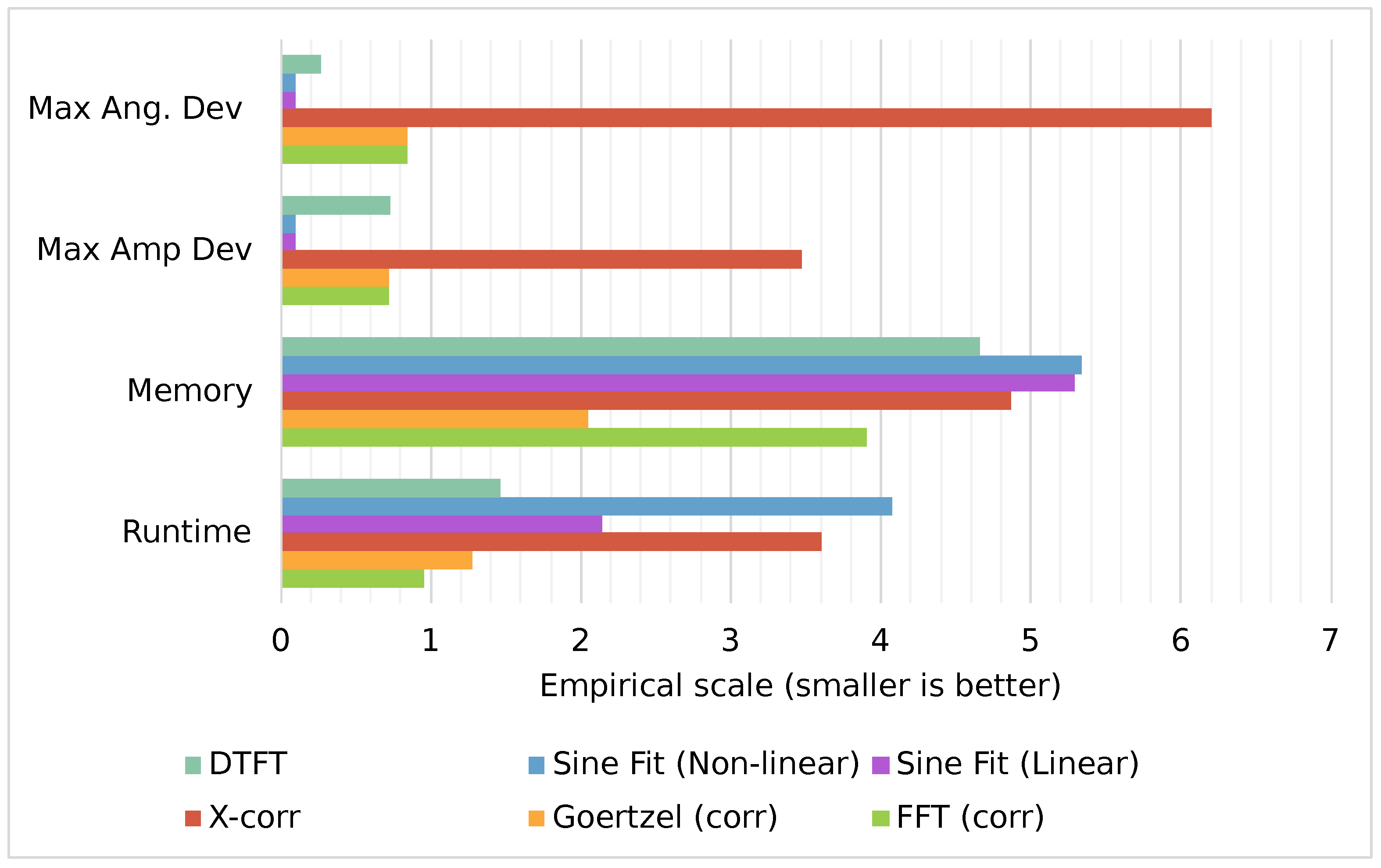
A comparison of the methods on an empirical scale is depicted in Figure 8. In this graph, the experimental data from the previous section from CMSIS-STM32 hardware acceleration are collected and are scaled with the help of $log(1+x)$. In this graph, smaller bars are better. The most accurate solution is sine-fit in both amplitude and phase accuracy. However, they suffer from long runtime. In this study, the linear least-squares sine-fit was deemed sufficient and enough to provide good results in a reasonable runtime. Yet, both sine-fit methods require expansive memory allocation that may not be available in all the microcontrollers. Therefore, FFT or Goerzel, both with correction are all-rounder solutions, could be used as an alternative, as they are both fast and memory-saving and have a good amplitude and phase accuracy. Alternatively, when phase accuracy is the most desired, DTFT could be used instead.

5. Conclusions

In this work, we compare AC signal analysis methods in terms of processing speed, memory consumption, amplitude, and phase accuracy for embedded solutions. First, we compare the computational complexity of all algorithms on a system without hardware acceleration. The memory consumption of each algorithm is then assessed, along with the expected accuracy in amplitude and phase determination. For validation, a test scenario is used, including four arbitrary sine waves. The AC signal analysis methods were first implemented in a Windows PC reference system using MATLAB and Visual C++. The results are compared with a native C program running on the STM32 and Teensy 3.6, with less hardware acceleration. Then a vectorized, hardware-accelerated CMSIS DSP program is implemented in STM32. It is shown that for native solutions, the Goertzel filter provides an all-rounder solution. In contrast, the FFT provides an all-rounder solution for the CMSIS DSP-based solution, given complete signals or barycenter correction technique for incomplete signals. Although, the phase accuracy lacks behind DTFT. However, when precision is desired in the expenses of execution time, linear least-squares sine fitting is the best solution, especially for prematurely truncated signals.

References

- Bouchaala, D.; Kanoun, O.; Derbel, N. High accurate and wideband current excitation for bioimpedance health monitoring systems. Measurement 2016, 79, 339–348. [Google Scholar] [CrossRef]
- Tröltzsch, U.; Kanoun, O.; Tränkler, H.R. Characterizing aging effects of lithium ion batteries by impedance spectroscopy. Electrochim. Acta 2006, 51, 1664–1672. [Google Scholar] [CrossRef]
- Shi, Q.; Kanoun, O. Wire fault location in coaxial cables by impedance spectroscopy. IEEE Sens. J. 2013, 13, 4465–4473. [Google Scholar] [CrossRef]
- Kallel, A.; Bouchaala, D.; Kanoun, O. Critical implementation issues of excitation signals for embedded wearable bioimpedance spectroscopy systems with limited resources. Meas. Sci. Technol. 2021, 32, 084011. [Google Scholar] [CrossRef]
- Fairweather, A.; Foster, M.; Stone, D. Battery parameter identification with pseudo random binary sequence excitation (prbs). J. Power Sources 2011, 196, 9398–9406. [Google Scholar] [CrossRef]
- Sanchez, B.; Vandersteen, G.; Bragos, R.; Schoukens, J. Basics of broadband impedance spectroscopy measurements using periodic excitations. Meas. Sci. Technol. 2012, 23, 105501. [Google Scholar] [CrossRef]
- Arbo, M.H.; Utstumo, T.; Brekke, E.; Gravdahl, J.T. Unscented multi-point smoother for fusion of delayed displacement measurements: Application to agricultural robots. MIC J. 2017, 38, 1–9. [Google Scholar] [CrossRef] [Green Version]
- Angelis, A.D.; Buchicchio, E.; Santoni, F.; Moschitta, A.; Carbone, P. Practical broadband measurement of battery EIS. In Proceedings of the 2021 IEEE International Workshop on Metrology for Automotive, MetroAutomotive 2021, Bologna, Italy, 1–2 July 2021; pp. 25–29. [Google Scholar] [CrossRef]
- Schoukens, J.; Pintelon, R.; Van Der Ouderaa, E.; Renneboog, J. Survey of excitation signals for FFT based signal analyzers. IEEE Trans. Instrum. Meas. 1988, 37, 342–352. [Google Scholar] [CrossRef]
- Duhamel, P.; Vetterli, M. Fast Fourier transforms: A tutorial review and a state of the art. Signal Process. 1990, 19, 259–299. [Google Scholar] [CrossRef] [Green Version]
- Lindahl, P.A.; Cornachione, M.A.; Shaw, S.R. A time-domain least squares approach to electrochemical impedance spectroscopy. IEEE Trans. Instrum. Meas. 2012, 61, 3303–3311. [Google Scholar] [CrossRef]
- Vaníček, P. Further development and properties of the spectral analysis by least-squares. Astrophys. Space Sci. 1971, 12, 10–33. [Google Scholar] [CrossRef]
- Zhang, J.Q.; Zhao, X.; Hu, X.; Sun, J. Sinewave fit algorithm based on total least-squares method with application to ADC effective bits measurement. IEEE Trans. Instrum. Meas. 1997, 46, 1026–1030. [Google Scholar] [CrossRef]
- Wang, W.; Chen, D.; Yao, W.; Chen, W.; Lu, Z. Fast lock-in amplifier electrochemical impedance spectroscopy for big capacity lead-acid battery. J. Energy Storage 2021, 40, 102693. [Google Scholar] [CrossRef]
- Gücin, T.N.; Ovacik, L. Online impedance measurement of batteries using the cross-correlation technique. IEEE Trans. Power Electron. 2019, 35, 4365–4375. [Google Scholar] [CrossRef]
- Cooley, J.; Tukey, J.W. An algorithm for the machine calculation of complex Fourier series. Math. Comput. 1965, 19, 297–301. [Google Scholar] [CrossRef]
- Johnson, H.; Burrus, C. An in-order, in-place radix-2 fft. In Proceedings of the ICASSP’84. IEEE International Conference on Acoustics, Speech, and Signal Processing, San Diego, CA, USA, 19–21 March 1984; Volume 9, pp. 473–476. [Google Scholar]
- Danielson, G.C.; Lanczos, C. Some improvements in practical Fourier analysis and their application to X-ray scattering from liquids. J. Frankl. Inst. 1942, 233, 435–452. [Google Scholar] [CrossRef]
- Thomas, L.H. Using a computer to solve problems in physics. In Applications of Digital Computers; Freiberger, W., Prager, W., Eds.; Ginn: Boston, MA, USA, 1963; pp. 44–45. [Google Scholar]
- Good, I.J. The interaction algorithm and practical Fourier analysis. J. R. Stat. Soc. Ser. B 1958, 20, 361–372. [Google Scholar] [CrossRef]
- Rader, C.M. Discrete Fourier transforms when the number of data samples is prime. Proc. IEEE 1968, 56, 1107–1108. [Google Scholar] [CrossRef]
- Bluestein, L. A linear filtering approach to the computation of discrete Fourier transform. IEEE Trans. Audio Electroacoust. 1970, 18, 451–455. [Google Scholar] [CrossRef] [Green Version]
- Pavan Kumar, K.; Priya Jain, R.K.S.; Rohith N, R.K. FFT Algorithm: A Survey. Int. J. Eng. Sci. 2013, 2, 22–26. [Google Scholar]
- Frigo, M.; Johnson, S.G. The design and implementation of FFTW3. Proc. IEEE 2005, 93, 216–231. [Google Scholar] [CrossRef] [Green Version]
- Goertzel, G. An algorithm for the evaluation of finite trigonometric series. Am. Math. Mon. 1958, 65, 34–35. [Google Scholar] [CrossRef] [Green Version]
- Tchegho, A.; Gräb, H.; Schlichtmann, U.; Mattes, H.; Sattler, S. Analyse und Untersuchung der Quantisierungseffekte beim Goertzel-Filter. Adv. Radio Sci. 2009, 7, 73–81. [Google Scholar] [CrossRef] [Green Version]
- Regnacq, L.; Wu, Y.; Neshatvar, N.; Jiang, D.; Demosthenous, A. A Goertzel Filter-Based System for Fast Simultaneous Multi-Frequency EIS. IEEE Trans. Circuits Syst. II Express Briefs 2021, 68, 3133–3137. [Google Scholar] [CrossRef]
- Biancacci, N. FFT Corrections for Tune Measurements. 2011. Available online: https://indico.cern.ch/event/132526/contributions/128902/attachments/99707/142376/Meeting1-06-11_FFT_corrections_for_tune_measurements.pdf (accessed on 22 April 2020).
- Oppenheim, A.V.; Schafer, R.W. Digital Signal Processing (Book); Research Supported by the Massachusetts Institute of Technology, Bell Telephone Laboratories, and Guggenheim Foundation; Prentice-Hall: Englewood Cliffs, NJ, USA, 1975. [Google Scholar]
- Zhang, J.Q.; Zhao, X.; Hu, X.; Sun, J. Sinewave fit algorithm based on total least-squares method. In Proceedings of the Quality Measurement: The Indispensable Bridge between Theory and Reality (No Measurements? No Science! Joint Conference-1996: IEEE Instrumentation and Measurement Technology Conference and IMEKO Tec, Brussels, Belgium, 4–6 June 1996; Volume 2, pp. 1436–1440. [Google Scholar]
- Taylor, J.; Hamilton, S. Some tests of the Vaníček method of spectral analysis. Astrophys. Space Sci. 1972, 17, 357–367. [Google Scholar] [CrossRef]
- National Instruments. 2015. Available online: https://download.ni.com/evaluation/pxi/Understanding%20FFTs%20and%20Windowing.pdf (accessed on 22 April 2020).
- Hu, Z.; Ramalingame, R.; Kallel, A.Y.; Wendler, F.; Fang, Z.; Kanoun, O. Calibration of an AC zero potential circuit for two-dimensional impedimetric sensor matrices. IEEE Sens. J. 2020, 20, 5019–5025. [Google Scholar] [CrossRef]
- Munjal, R.; Wendler, F.; Kanoun, O. Embedded wideband measurement system for fast impedance spectroscopy using undersampling. IEEE Trans. Instrum. Meas. 2019, 69, 3461–3469. [Google Scholar] [CrossRef]
- Brett, M. Sum of Sines and Cosines—Tutorials on Imaging, Computing and Mathematics. 2016. Available online: https://matthew-brett.github.io/teaching/sums_of_cosines.html (accessed on 26 December 2021).
Figure 1.
Influence of Incomplete Signal on the Single-side Discrete Fourier Analysis for a Sample 11 kHz Signal with a Complete Last Period, Quarter-complete Period (52% Spectral Leakage), and Half-complete Period (98% Spectral Leakage).
Figure 2.
(a) Time complexity of DTFT/Goertzel vs. FFT as a function of N and . (b) Time complexity of Sine-fit (linear) vs. FFT as a function of N and .
Figure 3.
(a) Memory usage of DTFT/Goertzel vs. FFT as a function of N and . (b) Memory usage of Sine-fit (linear) vs. FFT as a function of N and .
Figure 4.
(a) Full Comparison of the Different Signals. (b) A Zoom into the most Precise Methods.
Figure 5.
Figure 6.
Bump Chart of the AC signal analysis Methods Ordered by their speed in the Different Implementations.
Figure 7.
Amplitude spectrum using DFT on the test scenario.
Figure 8.
Methods comparison for implementation on a STM32 microcontroller with hardware acceleration.