Application of Hierarchical Agglomerative Clustering (HAC) for Systemic Classification of Pop-Up Housing (PUH) Environments

Abstract

This paper is the result of the first-phase, inter-disciplinary work of a multi-disciplinary research project (“Urban pop-up housing environments and their potential as local innovation systems”) consisting of energy engineers and waste managers, landscape architects and spatial planners, innovation researchers and technology assessors. The project is aiming at globally analyzing and describing existing pop-up housings (PUH), developing modeling and assessment tools for sustainable, energy-efficient and socially innovative temporary housing solutions (THS), especially for sustainable and resilient urban structures. The present paper presents an effective application of hierarchical agglomerative clustering (HAC) for analyses of large datasets typically derived from field studies. As can be shown, the method, although well-known and successfully established in (soft) computing science, can also be used very constructively as a potential urban planning tool. The main aim of the underlying multi-disciplinary research project was to deeply analyze and structure THS and PUE. Multiple aspects are to be considered when it comes to the characterization and classification of such environments. A thorough (global) web survey of PUH and analysis of scientific literature concerning descriptive work of PUH and THS has been performed. Moreover, out of several tested different approaches and methods for classifying PUH, hierarchical clustering algorithms functioned well when properly selected metrics and cut-off criteria were applied. To be specific, the ‘Minkowski’-metric and the ‘Calinski-Harabasz’-criteria, as clustering indices, have shown the best overall results in clustering the inhomogeneous data concerning PUH. Several additional algorithms/functions derived from the field of hierarchical clustering have also been tested to exploit their potential in interpreting and graphically analyzing particular structures and dependencies in the resulting clusters. Hereby, (math.) the significance ‘S’ and (math.) proportion ‘P’ have been concluded to yield the best interpretable and comprehensible results when it comes to analyzing the given set (objects n = 85) of researched PUH-objects together with their properties (n > 190). The resulting easily readable graphs clearly demonstrate the applicability and usability of hierarchical clustering- and their derivative algorithms for scientifically profound building classification tasks in Urban Planning by effectively managing huge inhomogeneous building datasets.

1. Introduction

1.1. Description of PUH-Environments–Web Search and Literature Survey

Pop-up housings (PUH) and temporary housing solutions (THS), respectively, can be characterized based on multiple aspects in terms of technical, architectural, infrastructural, economic, ecological, temporal and socio-cultural considerations as well as local conditions and contextual circumstances.

The following introductory statements are based on the general analysis of over 85 PUH/THS structures (see list ‘Collection of PUH-examples’ in Supplementary Materials) that have been researched and recorded/documented for later classification of PUH, which is the main aim of this paper. Moreover, the principal methodology of clustering, applicable to numerous similarly structured problems, is presented.

On the one hand, a rising need for affordable and sustainable THS, mainly in urban regions of developed countries, can be observed. This refers to a trend in the housing demand of young people, such as singles, students, workers and professionals, artists as well as young families. Rising requirements in the working environment concerning flexibility and mobility/stand-by duty, potentially lower-income situations and changing social developments/living conditions, among others, are triggering the subtle change in housing needs, particularly of younger generations. Such THS might play a role in the decarbonization of the building sector as well. Tumminia et al. [1] showed through LCA- and energy consumption simulations that for a high energy efficiency prefabricated building module for temporary housing, mainly consisting of fiber-reinforced plastic (FRP), the pre-use phase causes the most (72%) total environmental impacts compared to the use-phase (23%). Generally speaking, it is vital to use LCA methods to assess the overall energy and environmental performances of such temporary housing units [1].

Apart from housing units of solely architectural experiments and design studies, or artists’ visualization projects, there is also a market for (fairly extravagant) micro or tiny homes, ashore and afloat. These units are often single and provide (temporary) housing solutions for users who are seeking exclusive, often self-sustaining housing conditions, frequently being rather highly priced.

On the other hand, there are THS for people and user groups with a more ‘urgent or critical’ housing demand, such as socially underprivileged (local) people, lowest-income households, asylum seekers, refugees and homeless people, to name a few. These THS aim to provide more ‘basic’ housing/shelter options with high affordability and ease of build possibilities in mind.

In general, the global need for temporary housing is rising through the increasing severity of natural disasters, increase in number of climate refugees due to climate change and rapid urban population growth in developing countries [2].

THS for post-disaster situations seem to be analyzed most in the scientific literature [3,4,5,6]. Concerning a post-disaster temporary housing settlement, several contextual factors have to be considered, such as physical characteristics of the settlement, availability of vital services such as education, health and work, infrastructure services, accessibility to the temporary houses within the settlement, economic prospect of the temporary settlement as well as socio-cultural, educational and financial standards of the occupants, as pointed out by Abulnour [3]. Temporary accommodation in post-disaster situations is an issue that goes beyond the simple provisioning of housings since the whole space for the temporary settlement is important [4].

A considerable part of the provided THS is not produced in the affected region but in a different country, often neglecting local resources, such as building materials and labor workforce. Therefore, social problems and environmental degradation are often the consequence of false planning strategies (i.e., not considering the option of prolonged usage) and commonly require transition to permanent housing [4]. The lack of environmental, economic and social sustainability of temporary housing environments in post-disaster situations stems from poor governmental decision-making, lack of understanding of user’s needs and lack of realization and adaptability to local conditions, as discussed by Perrucci et al. [2].

As a consequence of the need to capture the great diversity of and to classify the researched and analyzed THS, a method being able to ‘cope’ with the heavy inter-disciplinary characteristics of the THS (i.e., mixed categorical and numerical data) had to be found. Therefore, a high amount of time has been spent for selecting, testing and refining a wide variety of already known clustering algorithms to come up with the best suitable clustering method in order to solve the aforementioned THS classification/structuring problem.

1.2. Data/Buildings Classification and Applied Clustering Algorithms

Throughout the past decade, data classification and clustering algorithms have been applied extensively in the fields of biology, engineering, information science, medical sciences as well as behavioral and social sciences, to name a few. Furthermore, cluster analysis has been widely used in many applications such as business intelligence, image pattern recognition, web search, biology and security [7]. The need for, and advantageous uses of, cluster analysis probably stem from the rising amount of readily available and processable big data and the urge to generate interpretable structures and usable classifications and correlations out of seemingly unstructured or highly heterogeneous datasets.

Concerning the classification and (technical) evaluation of buildings, various scientific studies have already been performed, mainly for energy consumption profiling [8,9,10,11,12,13,14] and assessing/improving energy efficiencies of different buildings [15,16] as well as benchmarking buildings [17,18,19,20,21,22,23]. A comprehensive review of performed cluster analyses in the building sector can be found in [15].

Throughout these performed studies (covering building topics), two methods for classification and clustering of data have proven themselves to be highly suitable and appropriate: hierarchical and k-means clustering algorithms. K-means is an iterative algorithm that divides a given dataset into k clusters by minimizing the sum of all squared Euclidian distances to the respective cluster centers (centroids to be chosen). Different ‘cluster quality indices’ are applied herein to obtain the optimal number of clusters, e.g., the ‘Davies and Bouldin’ and the ‘Silhouette’ indices. Grouping data into clusters so that objects within each specific cluster are very similar to each other but also very dissimilar to objects in other clusters requires distance measures (metrics based on indices of proximity) so that similarities and dissimilarities can be assessed correctly. Hierarchical data clustering results in a so-called ‘dendrogram’ (graphical clustering tree structure), which represents groupings of objects at specific (dis-) similarity levels. Which clustering algorithm to choose is a matter of specific properties, i.e., type and scale of the given dataset, for example. As a matter of fact, HAC can yield impressive and rather easily readable results concerning clustering and classification of general building information/datasets. In the following, the effective application of HAC on inhomogeneous data of PUH-environments is presented, leading to the obvious suggestion that HAC could be far more intensely used for building classification tasks in urban planning. For a detailed description of a novel clustering algorithm (k-CMM), especially suited to mixed numerical and categorical data, see e.g., Dinh et al. [24].

2. Methodology

2.1. Data Preparation–Data Type and Scale

Firstly, before initiating a cluster analysis through a specific clustering algorithm, an examination of the given dataset has to be performed in order to specify general clusterability (is cluster structure present?), data quality and data structure, as pointed out in Jain and Dubes [25]. The result of this first data analysis helps in choosing an appropriate distance metric, which is crucial for proper clustering results. In the present study, an analysis of over 85 PUH/THS (from now on referring to ‘objects’) has been performed, and a representative table with all (n) objects and over a hundred (d) attributes, describing them as holistically as possible, has been generated. This dataset is viewed as the (d x n) pattern matrix, where each row of this matrix represents a pattern, and each column denotes a feature/property. Features are categorized as binary; thus, each individual object does (Yes) or does not (No) contain a specific attribute. Binary features are best coded on a qualitative, nominal scale, e.g., (0, 1). Therefore, a suitable distance metric, measuring proximity between objects, must be chosen according to the data type and scale. The implemented metric for the (d x n) pattern matrix of PUH/THS results in the so-called proximity matrix [d(i, j)], containing the pairwise indices of proximity between the ith and jth object.

2.2. Cluster Analysis

2.2.1. Descriptions and Definitions of Application-Oriented Hierarchical Cluster Analysis (HCA)

As mentioned before, the proximity matrix describes the proximity between objects to be clustered using a problem-specific metric. It is the only, and therefore crucial, input to a clustering algorithm. The following application-oriented hierarchical clustering represents an exclusive (each object belongs to exactly one cluster with no overlapping), intrinsic (unsupervised, no a priori partition) and hierarchical (interlaces sequence of partitions) form of object classification. The following mathematical notations are explicitly taken from Jain et al. [26].

Hierarchical cluster analysis (HCA) is a procedure for transforming a defined proximity matrix into a sequence of interlaced partitions.

The n objects to be clustered are denoted by the set χ where x_i is the ith object:

$$\chi =\left\{x_1,x_2, x_3\dots .x_n \right\}$$

(1)

A partition, Γ of χ, divides χ into subsets $\left\{C_1,C_2\dots . C_m\right\}$, which satisfy the following expressions:

$$C_i\cap C_j=\varnothing$$

(2)

for all i and j from 1 to m, i ≠ j, where ∅ is the empty set,

$$C_1\cup C_2\cup \dots \cup C_m=\chi$$

(3)

the union of all clusters results in the total quantity of all n objects.

Thus, the hierarchical clustering algorithm yields a sequence of partitions in which each partition is nested into the next partition in the sequence. The process is repeated to form a sequence of nested clusters until a single cluster containing all n objects remains [26]. This approach is also called hierarchical agglomerative clustering (HAC). The visualization of the clustering results is obtained through a special type of tree structure called a dendrogram. A dendrogram consists of layers of nodes, each representing a cluster. Cutting a dendrogram horizontally creates a clustering [26]. Therefore, a suitable ‘cut-off’ criterion, described later in detail in the present chapter, must be defined in order to achieve an optimum number of clusters for a given set of objects.

Two specific hierarchical clustering methods can be distinguished, the single-link and the complete-link form. The sequences of clusterings created by these two methods depend on the proximities only through their rank order. Single-link clusters are characterized as maximally connected subgraphs, whereas complete-link clusters are maximally complete subgraphs [26]. In single-link clustering, the similarity of two clusters stems from the similarity of their most proximate similar objects. In complete-link clustering, the similarity of two clusters stems from the similarity of their most dissimilar objects. This diverse approach induces a different dendrogram; thus, a conscientious interpretation and analysis of the resulting clusterings are necessary.

2.2.2. Applied Clustering Technique

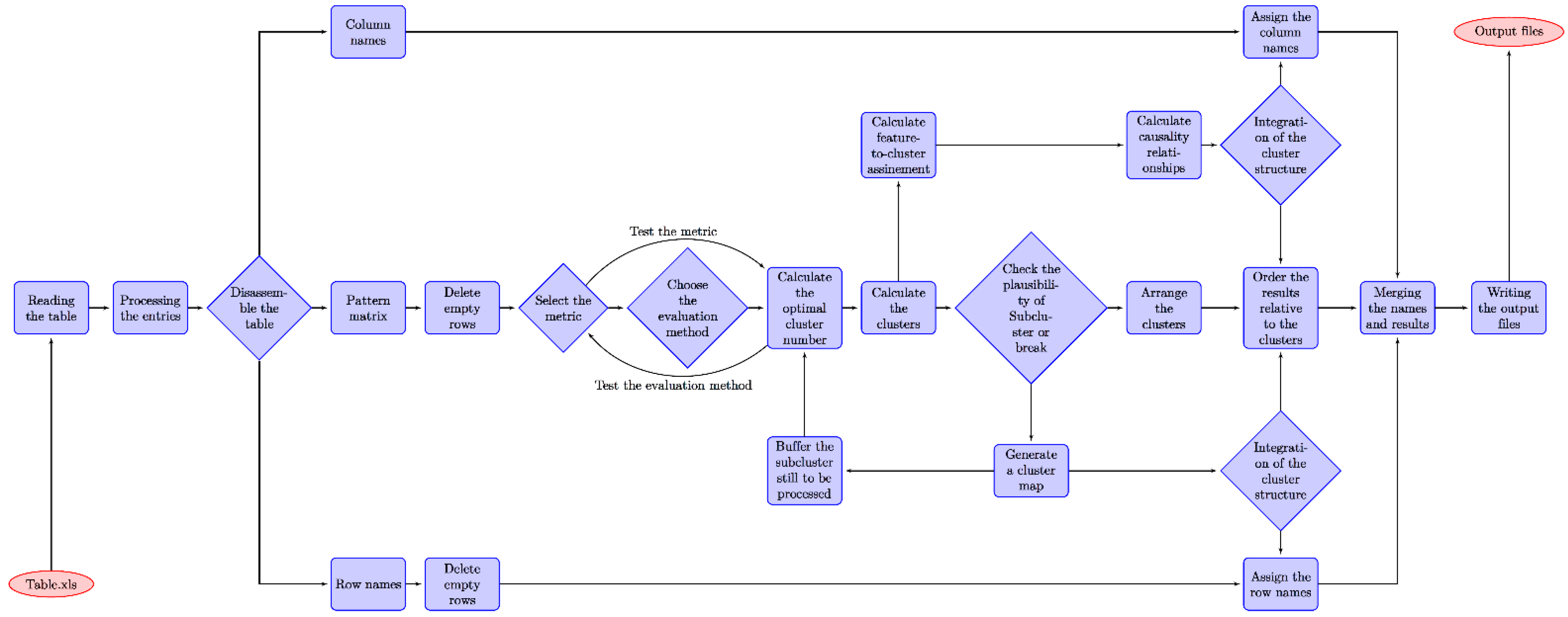
Figure 1 illustrates the step-by-step procedure performed to obtain the most suitable metric and cut-off criterion for the optimum number of clusters, thus calculating the final proximity matrix and displaying the obtained clusters through dendrograms. Accordingly, a final table with all objects (listed PUH) clustered by inconsistency coefficient and weighted match of columns has been generated. The following distance measures were included in this selection algorithm as depicted in Figure 1: basic, squared and standardized Euclidean distances, the City Block-, Minkowski-, Chebychev-, Mahalanobis-, Cosine-, Correlation-, Spearman-, Hamming- and Jaccard distances.

2.2.3. Measuring Dissimilarity: Proximity Index ‘Hamming Distance’ (Minkowski Metric)

Because of the underlying data nature and, as a result of the conducted selection algorithm, the most suitable and comprehensibly applicable metric out of all investigated proximity indices was chosen as the Minkowski proximity index d(i, k) between the ith and kth patterns, measuring dissimilarity d(i, i) = 0 for all i:

$$d\left(i, k\right)={\left({\displaystyle \sum }_{j=1}^d{\left|x_{ij}-x_{kj}\right|}^r\right)}^{\raisebox{1ex}{$1$}\!\left/ \!\raisebox{-1ex}{$r$}\right.}$$

(4)

where r ≥ 1.

Choosing r = 2 results in the Euclidean distance, the most common of the Minkowski metrics. For r = 1 and exclusively for binary features, the values are either 0 or 1. In this particular case, the Minkowski metric corresponds to the so-called ‘Hamming distance’. This metric is particularly useful for measuring differences and similarities as:

$$d\left(i, k\right)={\displaystyle \sum }_{j=1}^d\left|x_{ij}-x_{kj}\right|$$

(5)

with r = 1, see Equation (4).

2.2.4. Determining the Number of Clusters: Clustering Index ‘Calinski-Harabasz’-Criterion

In order to find the structure contained in the data, it is necessary to specify a suitable and ideal number of clusters for hierarchical clustering. To determine this number, the following evaluation criteria were analyzed in more detail, the Calinsky-Harabasz, Davies-Bouldin, Gap, Silhouette and Cut-off criteria for inconsistent data. A detailed description of the application of the Silhouette coefficient can be found in Dinh et al. [27].

The chosen Calinski-Harabasz index (known as Variance-Ratio criterion) is defined as the quotient of the degree of separation and compactness, using a normalization factor to limit the monotonous increase of the index with an increasing number of clusters. The Calinski-Harabasz index (CH-i) can therefore be written as:

$$CH\left(n\right)=\frac{S{S}_B}{S{S}_W}\times \frac{n-k}{k-1}$$

(6)

where n is the total number of data points (observed objects), k is the number of clusters, SS_B is the overall between (inter)-cluster variance or separation degree and SS_W is the overall within (intra)-cluster variance or compactness degree. Accordingly, the optimum number of clusters is achieved with the highest value of CH-i.

2.2.5. Deep Search

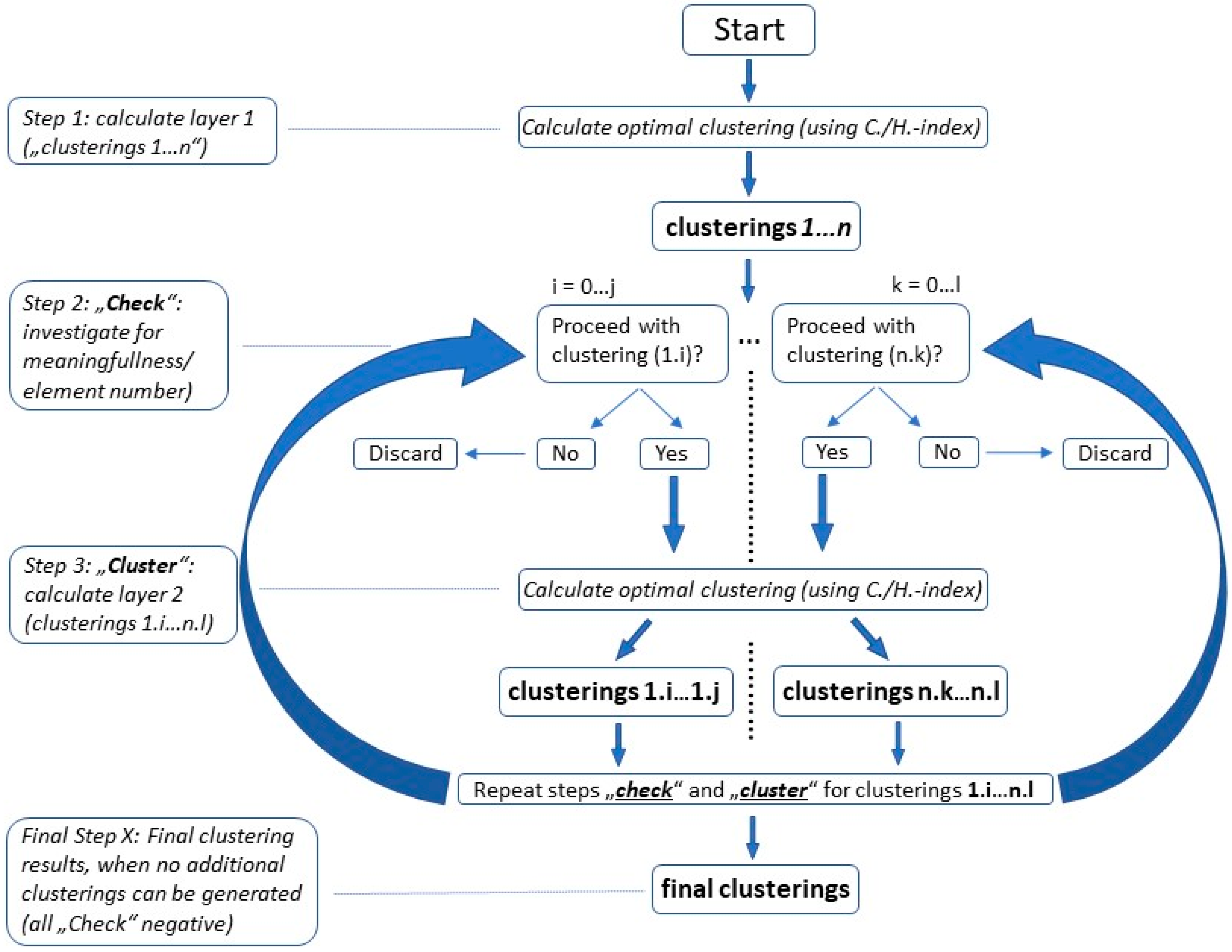
A depth-first search is used to identify any deeper structure in the data. The structure of the data is exposed recursively. In the first step, the optimal clustering is calculated. This step is called Layer 1. In the next step, the same procedure is applied again to each of the calculated clusters. After each new application, the calculated clusters are checked for meaningfulness with respect to the resulting clusters. If the result of the decomposition is mostly a cluster with only one element, this clustering step is discarded, and the search for this branch is stopped. If a cluster contains too few objects at the beginning of the new step, the process is stopped for this branch. Each new cycle is assigned to a new layer. The notation for this is Cluster-number_layer1-number_layer 2-…

For a more distinctive cluster analysis, and in order to obtain a deeper interpretation of the clustering results (assignments of an object (PUH) to a specific cluster), Bayesian rules are applied, and possible conclusions are drawn from there. Figure 2 shows the respective flow chart of the applied depth-first-search algorithm (showing procedure exemplary for the first two layers).

2.2.6. Limitations of Applied Method

As mentioned in the introductory section, there exist several proven distance (dissimilarity) measures as well as various clustering indices (cut-off criteria) to provide the optimum number of clusters for scattered, inhomogeneous data. The authors tried to conscientiously identify the most suitable metric and the best applicable clustering index according to the given datasets’ characteristics. Overall, several Matlab simulation test runs with different metrics and cut-off criteria were performed prior to settling on the mentioned Minkowski metric together with the ‘Calinski-Harabasz’-criterion. This choice, although evaluable and logically deducted, confines the possible clustering results, which potentially differ from each other when applying a specific metric and cut-off criterion. As a consequence, the provided clusterings in this paper must be considered as specific results from the application of an individually chosen and user-specific clustering technique, which might, albeit not heavily, differ from the results of other applied clustering algorithms.

2.3. Assessment

Two values were defined to evaluate whether a characteristic is meaningful with regard to a cluster. The first number evaluates how large the proportion of objects with this property is in the cluster. This value is referred to as P (proportion). The second number indicates how meaningful a characteristic of a cluster is in relation to all other clusters in the same level. This number is referred to as S (significance).

2.3.1. Proportion P_i

P_i describes the proportion of objects which possess the characteristic in relation to the number of objects in the considered cluster i.

$$P_i≔\frac{\#\left(Objects in the cluster which have the characteristic\right)}{\#\left(Objects in cluster\right)}$$

(7)

Equation (7) defines the proportion of the considered characteristic in the cluster with #, being the number of elements that have the described property and i being the cluster number.

2.3.2. Significance S_i

Significance S_i describes the likelihood that an object with an observed characteristic is in a particular cluster on the level under consideration. The Bayes theorem is used to define this value.

In the Bayesian approach, an observation is not allocated to a cluster with probability 1. The Bayesian approach generates cluster probabilities for each object. This is especially important for observations close to cluster boundaries [27].

Bayes’ theorem can be stated mathematically as follows, hereby defining the significance S_i:

$$S_i=P\left(A|B\right)=\frac{P\left(B|A\right) P\left(A\right)}{P\left(B\right)},$$

(8)

where A and B are events and P(B) ≠ 0.

P(A│B) and P(B│A) respectively denote the likelihood of event A (B) occurring, given that B (A) is true, called the conditional probability. P(A) and P(B) are the probabilities of observing events A and B independently of each other, called the marginal probability. Based on the definition, S_i describes a measure that, if an object has a characteristic, it is located in cluster i.

3. Results

3.1. Input Data for Clustering Algorithm

The presented methodology can be applied to all systems following the below-listed criteria. The input data for the verification of the model has been chosen from an evaluation of case examples for temporary living. The types of housing examples are called ‘objects’ within this publication. The objects have been selected within a scientific study on a global basis, whereas only objects in Vienna were physically visited. All other objects were only selected if comprehensive information could be accessed online. The described criteria were developed and selected within an interdisciplinary, scientific team of energy engineers, architects, waste management experts, sanitary engineers, landscape architects and special planning experts. Each criterion had to fulfill the condition that only ‘yes’ or ‘no’, and ‘existing’ or ‘not existing’ could be selected, e.g., one floor (yes/no), private kitchen (existing/not existing); where yes and no (as well as existing and not existing) were coded as 1 and 0, respectively.

Pattern and Proximity Matrix

As mentioned in the Introduction, 54 out of more than 85 analyzed objects (type of housing) were put together, i.e., listed as a complete dataset in a representative table with all (n) objects and nearly two hundred (d) properties, viewed as the (d x n) pattern matrix. Features were categorized as binary, and thus, each individual object did (marked with an X and being represented as 1) or did not (empty field being represented as 0) contain a specific property.

The data for the remaining objects were too incomplete, scattered or unclear to be included in the final table. The complete matrix is shown in the Supplementary Materials.

The pattern matrix represents the starting basis for all further clustering considerations and algorithmic calculations. Being rather large (see complete table with all objects and properties in ‘attachments’ to this paper), only a fragment of the matrix is depicted at this point, solely for illustrative purposes, showing all final objects, but only a fraction of all listed properties, see

Table 1. Extraction of (d x n)-pattern matrix as input table for further clustering calculations.

		(dxn)-Pattern Matrix
		Overall table (pattern matrix) of pop-up examples	A	A	A	A	A	A	A	A	A	A	B	B	B	B	C		C	C	C	C	C	C	C	C	C	C	C	C	C	C	C	C	C	C	C	C	C	C		D	D	D	D	D	D	D	D	D	D	D		E	E	E	E	E	E
		Consecutive Number	1	2	3	4	5	6	7	8	9	10	11	12	13	14	15		16	17	18	19	20	21	22	23	24	25	26	27	29	30	31	32	33	34	35	36	28	37		38	39	40	41	42	43	44	45	46	47	48		49	50	51	52	53	54
		ID-Number	43	51	19	58	45	9	32	44	6	49	61	37	16	10	62		46	63	31	5	13	47	28	40	38	39	12	11	34	27	15	29	30	33	23	4	64	17		52	22	25	50	8	14	53	60	18	41	42		54	59	48	21	65	3
	Object name	Properties	Weaving a Home	Base camp field hospital in Balukhali II	Emergency (..) center Hamburg	Cuvrybrache Berlin	Refugee Shelter Balukhali II	Instant (..) light weight /..) Munich	Better Shelter	Lifeshelter	Habitat for humanity	instant home	Wagendorf Lohmühle	Little Home Köln e.V.	Getaway House	Wohnwagon	FEMA Temporary housing units		EXO Emergency Shelters	Seven Skies Pop Up Hotel	micro compact home (m-ch)	Heijmans ONE	Sliding hub	Nader Khalili & Cal Earth Earth Buildings	BaleHouse	3D Printed home	3D Housing 05	BigDelta project	Prototype ME-01	Meme Meadows Experimental House	YMCA’s Y:Cube house	The Blob	Tanzania Rural Housing	Abaton casa transportable	Arc House	microHOME	Home Box	Passive house pop-up	Airclad Suffolk Pod	Concrete shelter Ahrweiler		Urban Rigger	Feel Home Taufkirchen	Pop-up dorms Seestadt Aspern	Wohncontainer Pfarre Rodaun	City Container Zürich	NYC Emergency Housing Prototype	Onagawa Temporary Container Housing	Startblok Riekerhaven	Cubity	Slim Building Siemensstraße	Holzmodule Podhaskygasse		Haus Liebhartstal	HAWI	Notunterkunft Primavesigasse	Pop-down Hotel	Sleepbox mobile hotel	Dwelling with SHED
1	6	free standing	x	x	x	x		x	x	x	x	x	x	x	x	x	x		x	x	x	x	x	x	x	x	x	x	x	x	x	x	x	x	x	x	x	x	x			x	x	x	x	x	x	x	x	x	x	x		x	x	x	x
2	3	newly built accomodation	x	x	x	x	x	x	x	x	x	x		x	x	x	x		x	x	x	x	x	x	x	x	x	x	x	x	x	x	x	x	x	x	x	x	x	x		x	x	x	x	x	x	x	x	x	x	x
3	180	unit transportable	x	x	x	x	x	x	x	x		x	x	x	x	x	x		x	x	x	x	x		x				x		x	x	x	x	x	x	x	x	x	x		x	x	x	x	x	x	x	x	x	x	x						x
4	4	prefabricated elements or modules	x	x	x		x	x	x	x		x	x	x	x	x	x		x	x	x	x	x		x				x	x	x	x	x	x	x	x	x	x	x	x		x	x	x	x	x	x	x	x	x	x	x						x
5	12	one floor	x	x	x	x	x	x	x	x	x	x	x	x	x	x	x		x	x	x		x	x		x	x	x	x	x	x	x	x	x	x	x		x	x	x					x					x
6	29	collectively used open space	x	x	x	x	x	x	x	x	x		x						x	x	x	x	x	.									x		x					x		x	x	x	x	x		x	x	x	x	x		x	x		x		x
7	31	access to shared toilet or similar	x	x	x			x	x	x	x		x						x	x																			x	x			x	x	x	x								x	x	x		x
8	10	industrial kitchen/field kitchen		x				x	.	.					x					x	x		x	.									x	x					x																	x	x	x
9	32	access to shared bathroom or washing area	.	x	x			x	x	x	x		x						x	x																			x	x			x	x	x	x								x	x	x		x
10	25	green land (former land use)		x	x		x		x	x																x		x												x			x									x
11	8	lightweight (rigid) materials				x		x	x	x	x	x	x	x	x	x	x		x	x	x	x	x		x	x	x	x	x	x	x	x	x	x	x	x	x	x	x			x	x	x	x	x		x	x	x		x						x
12	49	private kitchen/cooking facility	.				x				x		x	x	x	x			.		x	x	x		x	x	x	+	x	x	x	x		x	x	x	x	x				x					x	x	x		x	x
13	50	residential area (zoning plan)	.					x		.	.			x		x	x		.		x	x				x					x					x	x	x	x				x		x		x		x	x				x				x
14	52	one bed unit				x						x		x	x	x	x			x	x	x				x	x	x	x	x	x	x	x	x	x		x		x			x		x					x	x					x			x	x
15	54	primary material: wood				x							x	x	x	x							x		x					x	x			x	x	x	x	x					x	x						x		x			x			x	.
16	184	complete unit in more than one dwelling	x	x	x	x	x	x	x	x		x	x	x					x	x								x											x	x
17	185	one room only	x	x	x	x	x	x	x	x		x							x	x								x											x																			x
18	183	frameconstruction with lightweight walls	x	x	x	x	x	x	x	x	x
19	182	supported by poles and ropes		x	x	x	x	x
20	41	lightweight-textile (flexible) materials	x	x	x	x	x	x			x
21	139	innovative structure	x																																	x
22	121	rely on public toilette				x	x					x
23	122	rely on public bathroom				x	x					x
24	177	unit accessed by footpath		x	x	x	x	x	x	x	x	x							x	x	x	x																	x	x
25	187	unit with different qualities in the same PUE				x	x						x																										x										x									x
26	188	selfmade improvised dwelling				x							x
27	125	appropriation of open space (other than private)				x	x				x		x																																														.
28	126	expansion of unit during PUE life span					x				x		x
29	35	≥100 units on-site	.				x		x	.																																						x	x		x	x
30	186	tent units in a row (connected to each other)					x
31	39	connection to “buildings” on both sides					x																																																			x
32	142	expansion of PUE during PUE life span				x	x																																						x
33	84	mass shelter						x																																																x
34	175	lightweight ridig plastic							x	x																													x
35	16	primary material: coated paper										x
36	191	earth cellar (as refridgerator)											x
37	192	vermicomosting for organic waste streams											x
38	57	unit on wheels											x	x	x	x	x																																										x
39		one mobile unit											x	x	x	x	x
40	70	PUE consists of 1 unit (one unit on site)												x	x	x						x	x		x	x	x	x	x	x	x	x	x	x	x	x	x	x
41	178	Unit accessed on private plot												x	x	x				x			x	x	x	x	x	x	x	x	x	x	x	x	x	x	x	x	x
42	7	lockable unit(s)	.			.			x	x	x			x	x	x	x		x	x	x	x	x	x	x	x	x	x	x	x	x	x	x	x	x	x	x	x	x	x		x	x	x	x	x	x	x	x	x	x	x		x	x		x	x
43	63	unit has private toilet	.								x			x	x	x	x		.		x	x	x		x	x	x		x	x	x	x	x	x	x	x	x	x				x					x	x	x	x	x	x					x		.
44	62	unit has private bathroom	.												x	x	x		.		x	x	x		x	x	x		x	x	x	x	x	x	x	x	x	x				x					x	x	x	x	x	x					x		.
45	5	reversible (reusable) foundation															x		x	x	x		x	x	x	x	x	x	x	x	x	x	x	x	x	x	x	x	x	x			x		x			x		x
46	13	house with one unit per floor																	x	x	x	x	x	x	x	x	x	x	x	x	x	x	x	x	x	x	x	x	x	x
47	118	constructed on site only	x			x					x													x		x	x	x																											x	x	x
48	112	building ban with temporary building permit								.												x		.	x		x	x			x		x									x	.				x					x
49	128	3d printed																								x	x	x

.

A fragment of the proximity matrix [d(i, j)], containing the pairwise indices of proximity, i.e., the dissimilarity between the ith and jth object/feature, is presented in

Table 2. Proximity matrix [d(i, j)] (extr.), based on previously mentioned dissimilarity index/Minkowski metric.

	1	2	3	4	5	6	7	8	9	10	11	12	13	14	15
1	0.0000	0.1907	0.1753	0.2371	0.2165	0.2062	0.2165	0.1959	0.1649	0.2062	0.3041	0.2577	0.2474	0.3093	0.2680
2	0.1907	0.0000	0.1289	0.2732	0.1289	0.1289	0.1495	0.1495	0.1392	0.2113	0.3093	0.2113	0.2526	0.3144	0.2526
3	0.1753	0.1289	0.0000	0.2577	0.1753	0.0825	0.1340	0.1237	0.1443	0.1959	0.3247	0.2371	0.2268	0.2990	0.2371
4	0.2371	0.2732	0.2577	0.0000	0.2371	0.2577	0.2990	0.2887	0.2474	0.2474	0.2216	0.2371	0.2990	0.3196	0.2887
5	0.2165	0.1289	0.1753	0.2371	0.0000	0.1959	0.1856	0.1959	0.1546	0.2371	0.3041	0.2371	0.2680	0.3093	0.2887
6	0.2062	0.1289	0.0825	0.2577	0.1959	0.0000	0.1443	0.1237	0.1649	0.2165	0.3247	0.2371	0.2577	0.2887	0.2062
7	0.2165	0.1495	0.1340	0.2990	0.1856	0.1443	0.0000	0.0722	0.1443	0.1753	0.3144	0.2165	0.2165	0.2784	0.2474
8	0.1959	0.1495	0.1237	0.2887	0.1959	0.1237	0.0722	0.0000	0.1237	0.1856	0.3041	0.1959	0.2268	0.2577	0.2268
9	0.1649	0.1392	0.1443	0.2474	0.1546	0.1649	0.1443	0.1237	0.0000	0.2062	0.2835	0.1753	0.2062	0.2577	0.2165
10	0.2062	0.2113	0.1959	0.2474	0.2371	0.2165	0.1753	0.1856	0.2062	0.0000	0.3351	0.1753	0.1546	0.2784	0.2268
11	0.3041	0.3093	0.3247	0.2216	0.3041	0.3247	0.3144	0.3041	0.2835	0.3351	0.0000	0.2732	0.3144	0.2938	0.3144
12	0.2577	0.2113	0.2371	0.2371	0.2371	0.2371	0.2165	0.1959	0.1753	0.1753	0.2732	0.0000	0.1237	0.1546	0.1649
13	0.2474	0.2526	0.2268	0.2990	0.2680	0.2577	0.2165	0.2268	0.2062	0.1546	0.3144	0.1237	0.0000	0.1753	0.1856
14	0.3093	0.3144	0.2990	0.3196	0.3093	0.2887	0.2784	0.2577	0.2577	0.2784	0.2938	0.1546	0.1753	0.0000	0.1856
15	0.2680	0.2526	0.2371	0.2887	0.2887	0.2062	0.2474	0.2268	0.2165	0.2268	0.3144	0.1649	0.1856	0.1856	0.0000
16	0.1907	0.2062	0.1804	0.3041	0.2629	0.2113	0.1804	0.2010	0.2113	0.1804	0.3299	0.2629	0.2216	0.3247	0.2113
17	0.2423	0.2165	0.1701	0.2835	0.2938	0.1804	0.2010	0.1804	0.2216	0.2113	0.2990	0.2216	0.2320	0.2938	0.1907
18	0.2732	0.2268	0.1907	0.3144	0.2835	0.2113	0.2216	0.2010	0.2010	0.2216	0.3299	0.1907	0.1907	0.2113	0.1186
19	0.2990	0.2629	0.2474	0.3093	0.3093	0.2474	0.2474	0.2268	0.2268	0.2268	0.3351	0.1959	0.2165	0.2062	0.1649
20	0.2577	0.2526	0.2474	0.3196	0.3093	0.2474	0.2371	0.2371	0.2474	0.2062	0.3557	0.2062	0.1443	0.2165	0.1546
21	0.1856	0.2320	0.2474	0.2474	0.2165	0.2577	0.2268	0.2062	0.1546	0.2474	0.2835	0.1856	0.2474	0.2577	0.2062
22	0.2784	0.2835	0.2680	0.3402	0.3093	0.2887	0.2474	0.2474	0.2371	0.1959	0.3763	0.1959	0.1340	0.2062	0.1856
23	0.2938	0.2990	0.2526	0.3454	0.3351	0.2629	0.2526	0.2423	0.2320	0.1907	0.3711	0.2113	0.1598	0.2113	0.1907
24	0.2629	0.2990	0.2526	0.3454	0.3351	0.2835	0.2526	0.2423	0.2320	0.1804	0.3814	0.2320	0.1598	0.2423	0.1907
25	0.2629	0.2680	0.2216	0.3247	0.3041	0.2629	0.2113	0.2216	0.2113	0.1598	0.3711	0.2113	0.1495	0.2732	0.2320
26	0.2216	0.2577	0.2526	0.3454	0.2835	0.2732	0.2320	0.2113	0.1907	0.2010	0.3505	0.1907	0.1495	0.2216	0.1907
27	0.2680	0.3041	0.2784	0.2990	0.3299	0.2887	0.2577	0.2371	0.2474	0.2474	0.3247	0.1856	0.1753	0.1856	0.2165
28	0.2990	0.2526	0.2268	0.3196	0.2887	0.2165	0.2268	0.2165	0.2165	0.2062	0.3557	0.1443	0.1546	0.1546	0.1134
29	0.2938	0.2577	0.2320	0.2835	0.3041	0.2526	0.2423	0.2216	0.2320	0.1907	0.3299	0.1598	0.1701	0.1701	0.1392
30	0.2680	0.2320	0.2371	0.3093	0.2887	0.2474	0.2165	0.1753	0.2062	0.2165	0.3454	0.1546	0.1753	0.2062	0.2165
31	0.2577	0.2526	0.2268	0.2784	0.2680	0.2577	0.2062	0.2062	0.2062	0.1856	0.3247	0.1340	0.0722	0.1753	0.1753
32	0.2629	0.2474	0.2629	0.3041	0.2732	0.2629	0.2010	0.2216	0.2216	0.2216	0.3196	0.1495	0.1495	0.1598	0.1907
33	0.2938	0.3299	0.2732	0.3454	0.3454	0.2938	0.2835	0.2526	0.2732	0.2629	0.3711	0.2113	0.2113	0.1804	0.1804
34	0.3041	0.2990	0.2629	0.3041	0.3247	0.2629	0.2835	0.2526	0.2423	0.2423	0.3402	0.1495	0.1907	0.1598	0.1495
35	0.2990	0.2835	0.2371	0.3299	0.2990	0.2474	0.2577	0.2268	0.2268	0.2371	0.3454	0.1649	0.1649	0.1340	0.1340
36	0.2577	0.2320	0.1856	0.2680	0.2990	0.1959	0.2371	0.2062	0.2371	0.2371	0.2938	0.2268	0.2474	0.2371	0.1753
37	0.2526	0.1753	0.1289	0.3351	0.2526	0.1392	0.1495	0.1289	0.2010	0.2320	0.3299	0.2526	0.2423	0.3041	0.2113
38	0.3351	0.3093	0.3041	0.3557	0.3557	0.2938	0.3144	0.2835	0.2835	0.3144	0.3299	0.2732	0.2835	0.2835	0.2113
39	0.3093	0.2423	0.1753	0.3402	0.2784	0.1753	0.2062	0.1649	0.2268	0.2680	0.3454	0.2371	0.2474	0.2474	0.1856
40	0.3093	0.2216	0.2371	0.3196	0.3093	0.2165	0.2268	0.2062	0.2371	0.2680	0.3247	0.2268	0.2577	0.2474	0.1959
41	0.3196	0.2216	0.2062	0.3299	0.2887	0.1753	0.2165	0.1856	0.2474	0.2887	0.3144	0.2577	0.2887	0.2887	0.1959
42	0.2887	0.2423	0.1856	0.3299	0.2784	0.1753	0.2165	0.1753	0.2165	0.2577	0.3454	0.2577	0.2474	0.2784	0.2165
43	0.2835	0.2474	0.2320	0.3660	0.2835	0.2423	0.2320	0.2113	0.2216	0.2629	0.3814	0.2216	0.2320	0.2320	0.1701
44	0.2887	0.2629	0.2371	0.3505	0.2680	0.2474	0.2371	0.2062	0.2062	0.2680	0.3454	0.2371	0.2371	0.2371	0.1340
45	0.3505	0.3041	0.2680	0.3402	0.3093	0.2577	0.2784	0.2577	0.2784	0.2990	0.3351	0.2577	0.2577	0.2784	0.1649
46	0.3247	0.2784	0.2629	0.3247	0.3351	0.2629	0.2629	0.2526	0.2835	0.2835	0.3196	0.2423	0.2423	0.2423	0.1598
47	0.3196	0.2835	0.2680	0.3402	0.2990	0.2577	0.2784	0.2474	0.2577	0.2990	0.3866	0.2474	0.2577	0.2371	0.1959
48	0.3196	0.2732	0.2577	0.3505	0.2990	0.2474	0.2680	0.2371	0.2268	0.2990	0.3557	0.2371	0.2474	0.2165	0.1856
49	0.3454	0.2887	0.2526	0.3660	0.3351	0.2320	0.2835	0.2526	0.2732	0.3247	0.3711	0.3041	0.3247	0.3247	0.2526
50	0.3505	0.2938	0.2887	0.3608	0.3608	0.2474	0.2887	0.2680	0.2990	0.3505	0.3454	0.3093	0.3299	0.3711	0.2887
51	0.2835	0.2577	0.2113	0.3454	0.3247	0.2113	0.2732	0.2526	0.2423	0.2526	0.3814	0.2732	0.2629	0.3247	0.2629
52	0.3041	0.2990	0.2526	0.3557	0.3351	0.2732	0.2835	0.2526	0.2526	0.2938	0.4124	0.2835	0.2423	0.2629	0.2320
53	0.3093	0.2629	0.2268	0.3402	0.3196	0.2371	0.2784	0.2371	0.2784	0.2784	0.3144	0.2577	0.2680	0.3093	0.2474
54	0.2938	0.2680	0.2320	0.3351	0.3454	0.2526	0.2629	0.2526	0.2526	0.2835	0.3402	0.2629	0.2732	0.3144	0.2216

for illustrative purposes only. As can be seen in Table 2, the diagonal entries of the proximity matrix can be ignored since all patterns are assumed to have the same degree of dissimilarity (namely zero) with themselves. One can also identify the symmetry of the proximity matrix since all pairs of objects have the same proximity index, independent of the order in which they are stated.

3.2. Visualization of Clustering Results

3.2.1. Overview of the Resulting Structuring

Table 3. Overview of the resulting PUH-environment.

Layer 1	Layer 2	Layer 3	Name of the PUH-Environment
Layer I Cluster 2	Layer II Cluster 2-1	C2-1-3	Haus Liebhartstal
			HAWI
			Dwelling with SHED
			Sleepbox mobile hotel
		C2-1-2	Notunterkuft Primavesigasse
			Pop-down Hotel
		C2-1-1	Cubity
			Pop-up dorms Seestadt Aspern
			City Container Zürich
			Wohncontainer Pfarre Rodaun
	Layer II Cluster 2-2	C2-2-3	Slim Building Siemensstraße
			Holzmodule Podhaskygasse
			Onagawa Temporary Container Housing
			NYC Emergency Housing Prototype
			Urban Rigger
			Startblok Rikerhaven
			Feel Home Taufkirchen
		C2-2-2	Concrete shelter Ahrweiler
			Airclade Suffolk Pod
			FEMA Temporary housing units
			Micro compact home (m-ch)
			Heijmans One
			Sliding hub
			Bale House
			The Blob
			YMCA’s: Cube house
			Passive house pop-up
			Microhome
			Home Box
			Wohnwagon
			Little Home Köln e.V.
			Getaway House
			Abaton casa transportable
			Meme meadows Experimental House
			Arc House
			Tanzania Rural Housing
			Prototype ME-01
		C2-2-1	Seven Skies Pop Up Hotel
			3D Housing 05
			3D Printed home
			Big Delta project
Layer I Cluster 1			Instant home
			EXO Emergency Shelters
			Weaving a Home
			Nader Khalili & Cal Earth Buildings
			Habitat for humanity
			Lifeshelter
			Better Shelter
			Emergency (…) center Hamburg
			Instant (…) lightweight...) Munich
			Base camp field hospital in Balukhali II
			Refugee Shelter Balukhali II
			Cuvrybrache Berlin
			Wagendorf Lohnmühle

gives a graphical overview of the resulting clustering of the PUH environment. The distribution of clusters in the individual layers, as well as the assignment of the THS to the individual clusters, are clearly visible. Moreover, it can be seen that Cluster 1 within Layer 1 could not be broken down further. However, enlarged sample sizes could result in a meaningful clustering of the THS samples in Layer 2. The former Cluster 1 could be implemented into a new cluster structure. Finally, the number of layers is not limited to three. In the corresponding case study, the mathematical modeling did not result in any further, meaningful sub-clusters. Again, an enlarged sample size could lead to different results, eventually leading to a higher number of layers. Summarizing, after a correct selection of states for each criterion, the mathematical solution shows the clusters as well as the number of layers.

3.2.2. Proximity Dendrogram

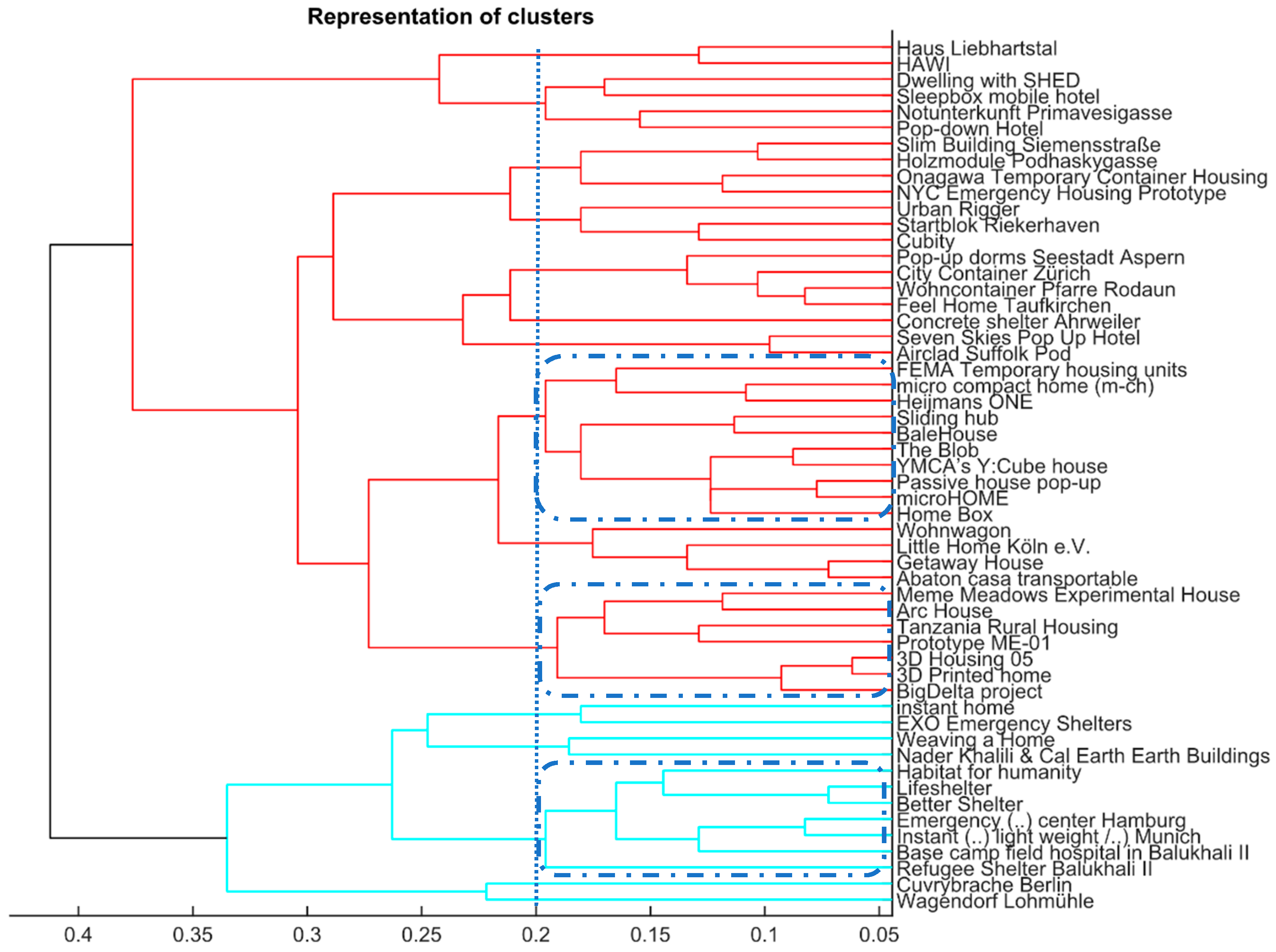
As mentioned above, a dendrogram represents the graphical form of clusterings, either in single-link or complete-link form. Moreover, a dendrogram yields the nested grouping of patterns and similarity levels at which groupings change [26].

Figure 3 represents the complete-link dendrogram for the input data. Two major clusters can be identified (differentiated by color); The length of the various bars describes the dissimilarity or proximity between various objects using the specified metric. As can be seen in Figure 3 (marked by dotted blue line), several sub-clusters can be formed and visualized when using a specific clustering index as ‘stop criterion’ (e.g., 0.2).

4. Discussion

4.1. Bar Plots–Feature-To-Cluster Assignment

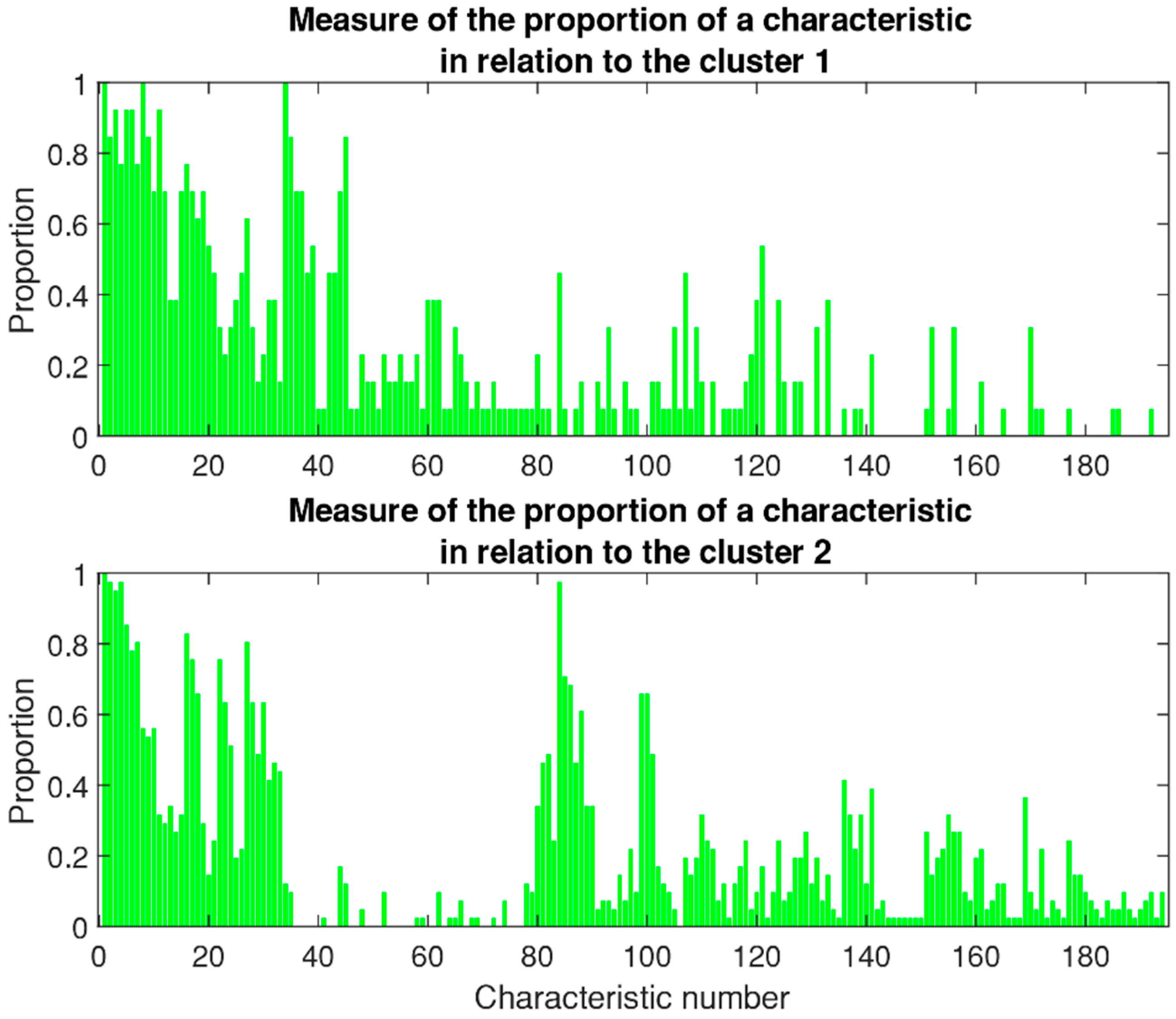
In the following, typical results of the mathematical modeling are presented. The selected types of illustration are typical examples of how those results can be presented. Figure 4 shows the proportion as calculated according to the above-derived equation for each characteristic element. The frequency of occurrence is normalized to one, which means that one represents 100% of examples in the cluster having the considered characteristic, whereas 0 means 0% of the examples show this specific characteristic. Thus, the values, and especially the shape, of the graphs indicate the importance of specific characteristics for each cluster. It is straightforward to create illustrations, as shown in Figure 4 for each cluster, to compare the significance of each group of characteristics with each other. These illustrations help the experts who provide the initial data to neutrally evaluate the results.

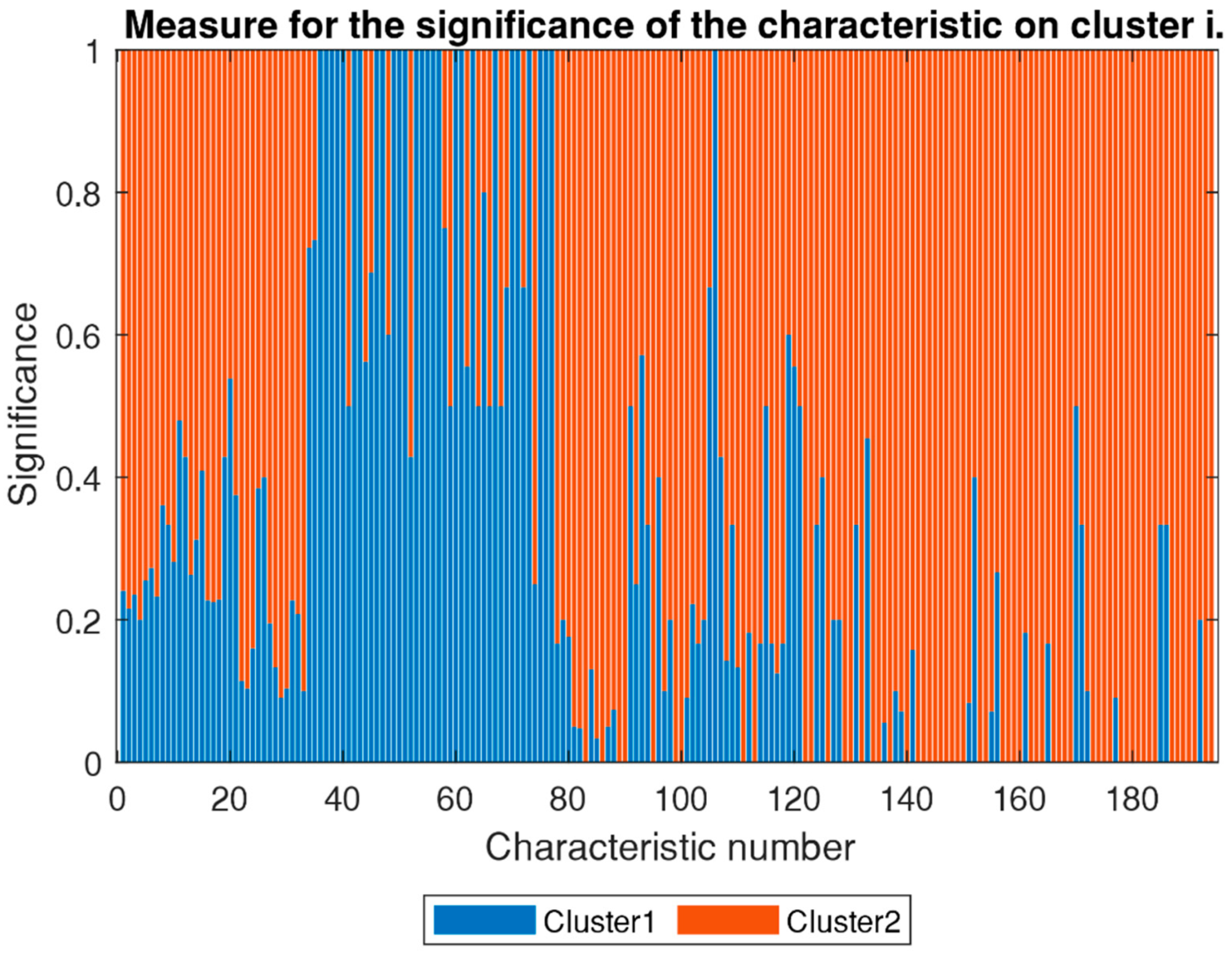
In Figure 5, the significance of each characteristic in a cluster in relation to the so-called parent cluster is shown. Based on the investigated cluster, a specific number ‘i’ of sub-clusters results from the calculations. For simplicity, again, only two sub-clusters are used in the explanatory illustrations. A significance of ‘1’ means that the specific characteristic is only present in one sub-cluster of all sub-clusters extracted out of one parent cluster. A significance of ‘0’ means that this characteristic is not existing in the sub-cluster ‘i’. Again, this type of illustration helps to group the classifications and allows a graphical evaluation of the results based on the mathematical modeling. This allows a dispassionate evaluation of the results of the initial classification of the example cases. In comparison to the classical evaluation of large groups of objects, these findings and the selected methods of presentation are big advantages to avoid misjudgments by the experts.

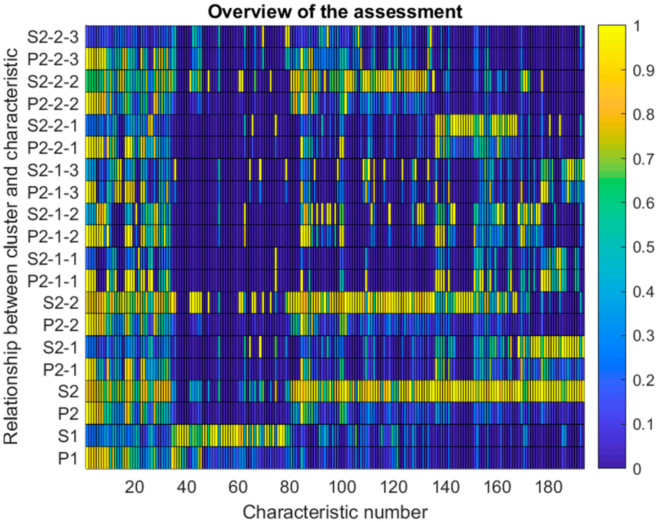
Figure 6 gives a graphical overview of the whole assessment of data, including the conciseness, given as proportion, and significances of each characteristic number for several layers of classes (parent cluster down to each layer of sub-clusters). Again, the values are normalized to ‘1’, representing all cases in the corresponding cluster, and ‘0’, meaning no proportion/significance. The visual presentation of the results of mathematical modeling can be used to distinguish relevance. If both criteria (proportion and significance) are high for a specific characteristic within a specific cluster, it can be stated that this characteristic is relevant for the assignment of objects into the cluster. If only the proportion is high, this means that the characteristic criteria are relevant for the cluster but should not be exclusively assigned. In other words, many objects within the observed cluster possess specific characteristics, but other objects in other clusters possess this characteristic as well. Vice versa, it can be stated if only the significance is high, this means that the characteristic is the reason for assigning the object to the cluster, but many other objects in the same cluster do not possess this characteristic.

Summarizing, the combination of proportion and significance, and especially their gradient between the different layers of clusters (parent cluster, sub-clusters, sub-sub-clusters, …), allows a description for each specific cluster. Based on the graphical presentation, which is created automatically out of the results of the mathematical modeling, the experts can easily determine the relations between the list of objects.

4.2. Interpretation

As an example, properties Nr. 1 (‘residential use’) and Nr. 2 (‘embedded in formal setting’) generally represented descriptive characteristics. Both exhibited a proportion of p = 1 in all clusters and layers. Whereas the significance S was clearly below 1 (S << 1), meaning that the specific PUH-objects, namely dwelling forms, are very homogeneously distributed in the particular clusters.

It is possible to identify properties that are representative of a particular cluster, i.e., properties that are relevant for the assignment of a PUH-object to a particular cluster (classification). Properties Nr. 36 (‘space-saving transport’), Nr. 37 (‘frame construction with lightweight walls’), Nr. 38 (‘supported by poles and ropes’) and Nr. 58 (‘embedded in informal setting’) exhibited relevance for their specific clusters, i.e., their significance S was S = 1, and their proportion P was rather high.

Properties that are strongly descriptive, i.e., relevant for classification/assignment to particular clusters, can be explicitly found for Cluster 2 and its subclusters. Property Nr. 87 (‘thermal insulation’), Nr. 88 (‘reversible/reusable foundation’), Nr. 99 (‘unit connected to centralized water supply’), 100 (‘unit has sewage connection’) and Nr. 101 (‘house with one unit per floor’) were the most significant characteristics.

5. Conclusions

5.1. Final Classification Remarks

5.1.1. General

At least 80% of all analyzed objects (n = 54) were free-standing, all-year-round habitable, newly built and transportable structures made of prefabricated elements in modular design. Nearly all (95%) were officially built and positioned according to legal zoning formalities, although ‘illegally’ built pop-up housings are obviously less likely to be registered and/or well-documented in scientific literature.

5.1.2. Building Flexibility

Very few (~7%) objects exhibited appropriation of public open space, while, simultaneously, these pop-up housings seemed to be readily expandable during their specific life span. The majority (93%) of the analyzed objects were not designed with a potential expansion in mind as one could suggest regarding the changing needs of their users.

5.1.3. Environment

A vast majority (~75%) of the investigated pop-up housings were inhabited all-year-round, excluding emergency, short-term and basic shelters, as well as solely experimental setups. Those objects that are being used throughout the year were most commonly based in urban environments. It is essentially the micro-compact and 3D-printed housings, as well as structures on wheels, such as mobile homes, that are not necessarily built or placed in urban regions, although the target area for compact (3D build) housing concepts is definitely the urban region as well. To date, micro-compact and 3D-printed housing concepts remain as prototypes without real-life applications, although this could change rather quickly depending on progress in technology and material advances.

5.1.4. Infrastructure/Technical Layout

Although some (~10%) of the investigated objects, like refugee and emergency shelters, only have access to a public bathroom and toilet, most of the analyzed pop-up housing structures do incorporate in-house sanitary facilities, even if about 40% of these objects have only shared access to a toilet/bathroom. Those housings with private sanitary rooms (toilet/bathroom) typically also incorporate a private kitchen or cooking facility. A tendency towards shared cooking facilities can be observed in shared housing, e.g., student dorms/halls and flat-sharing solutions for migrants and asylum seekers.

Apparently, it is very difficult to obtain detailed and reliable data on energy supply, i.e., thermal energy for heating/DHW purposes, as well as supply of electrical energy and sufficient data on (waste) water infrastructure. However, the results from the performed cluster analysis reveal that pop-up housings claiming energy autarchy also (have to?) operate water purification plants. This suggests that ‘overall autarchy’ is basically a need in remote areas where public energy and water supply are not easily accessible.

The more basic pop-up structures are seldom connected to the power grid or centralized water supply and have a sewage connection or even municipal waste collection. These infrastructural attributes, in most cases, only apply to more solidly built and profoundly positioned housings, which are often owned by their inhabitants.

5.1.5. Construction

The need and justification for building an underground cellar is found only in a few (~10%) permanently built objects. Above all, these structures are mostly used for temporary housing under rental conditions (e.g., temporary hotels).

Nearly 60% of the analyzed objects, particularly micro-compact and 3D-printed housings, are based on a reversible, i.e., reusable foundation on a private plot. Apparently, because of this, these typically modular structures are also built according to the one-unit-per-floor concept and often, due to the static structure and used materials, do not incorporate a second floor or multi-unit-layouts.

The more urgent the need for accommodation, as is the case for migrants and refugees, the more straightforward and faster it is to build or prepare the pop-up housings. Therefore ‘simple and quick’ solutions like basic shelters, modified containers or converted multi-use buildings are preferred. Shelters and ‘camps’ are necessarily realized by incorporating lightweight walls for frame construction, often supported by poles/ropes and by using lightweight materials, i.e., textile and/or flexible, which can be transported easily and in a space-saving way.

About 75% of all investigated objects used lightweight, rigid materials for construction, whereas two-thirds of the analyzed structures consisted of a single housing unit with one floor. Sixty percent of the documented pop-up housings incorporated units that can be reused or recycled, which implies simple modular construction, removable foundations and recyclable materials. About 37% of the documented objects use wood as the primary building material and thermal insulation with conventional insulators.

5.2. Final Conclusions

This paper intends to showcase the structured and very effective application of hierarchical clustering algorithms to a set of seemingly inhomogeneous objects of pop-Up environments/temporary housing solutions from around the globe under interdisciplinary consideration. It tries to identify the necessary steps, i.e., the inherent procedure to be followed for performing effective and productive clustering of data. Furthermore, the authors intended to illustrate several possible options for analyzing and interpreting scattered information/data in detail by using hierarchical clustering algorithms and their derivative considerations and calculations, respectively. Finally, conclusive classification remarks are given, pointing out in detail the similarities and differences of the clustered set of PUE objects.

This procedure can be applied to all kinds of data to allow a neutral presentation of the connections between datasets. Thus, interpretation of connection clustering within large datasets can be performed objectively.

References

- Tumminia, G.; Guarino, F.; Longo, S.; Ferraro, M.; Cellura, M.; Antonucci, V. Life cycle energy performances and environmental impacts of a prefabricated building module. Renew. Sustain. Energy Rev. 2018, 92, 272–283. [Google Scholar] [CrossRef]
- Perrucci, D.V.; Vazquez, B.A.; Aktas, C.B. Sustainable Temporary Housing: Global Trends and Outlook. Procedia Eng. 2016, 145, 327–332. [Google Scholar] [CrossRef] [Green Version]
- Abulnour, A.H. The post-disaster temporary dwelling: Fundamentals of provision, design and construction. HBRC J. 2014, 10, 10–24. [Google Scholar] [CrossRef] [Green Version]
- Félix, D.; Monteiro, D.; Feio, A. Estimating the needs for temporary accommodation units to improve pre-disaster urban planning in seismic risk cities. Sustain. Cities Soc. 2020, 61, 102276. [Google Scholar] [CrossRef]
- Arslan, H. Re-design, re-use and recycle of temporary houses. Build. Environ. 2007, 42, 400–406. [Google Scholar] [CrossRef]
- Potangaroa, R. Sustainability by Design: The Challenge of Shelter in Post Disaster Reconstruction. Procedia—Soc. Behav. Sci. 2015, 179, 212–221. [Google Scholar] [CrossRef] [Green Version]
- Mora, D.; Fajilla, G.; Austin, M.C.; de Simone, M. Occupancy patterns obtained by heuristic approaches: Cluster analysis and logical flowcharts. A case study in a university office. Energy Build. 2019, 186, 147–168. [Google Scholar] [CrossRef]
- Wei, Y.; Zhang, X.; Shi, Y.; Xia, L.; Pan, S.; Wu, J.; Han, M.; Zhao, X. A review of data-driven approaches for prediction and classification of building energy consumption. Renew. Sustain. Energy Rev. 2018, 82, 1027–1047. [Google Scholar] [CrossRef]
- Deb, C.; Lee, S.E. Determining key variables influencing energy consumption in office buildings through cluster analysis of pre- and post-retrofit building data. Energy Build. 2018, 159, 228–245. [Google Scholar] [CrossRef]
- Yang, J.; Ning, C.; Deb, C.; Zhang, F.; Cheong, D.; Lee, S.E.; Sekhar, C.; Tham, K.W. K-Shape clustering algorithm for building energy usage patterns analysis and forecasting model accuracy improvement. Energy Build. 2017, 146, 27–37. [Google Scholar] [CrossRef]
- Li, K.; Ma, Z.; Robinson, D.; Ma, J. Identification of typical building daily electricity usage profiles using Gaussian mixture model-based clustering and hierarchical clustering. Appl. Energy 2018, 231, 331–342. [Google Scholar] [CrossRef]
- Heidarinejad, M.; Dahlhausen, M.; McMahon, S.; Pyke, C.; Srebric, J. Cluster analysis of simulated energy use for LEED certified U.S. office buildings. Energy Build. 2014, 85, 86–97. [Google Scholar] [CrossRef] [Green Version]
- Pieri, S.P.; Tzouvadakis, I.; Santamouris, M. Identifying energy consumption patterns in the Attica hotel sector using cluster analysis techniques with the aim of reducing hotels’ CO2 footprint. Energy Build. 2015, 94, 252–262. [Google Scholar] [CrossRef]
- Ma, Z.; Yan, R.; Li, K.; Nord, N. Building energy performance assessment using volatility change based symbolic transformation and hierarchical clustering. Energy Build. 2018, 166, 284–295. [Google Scholar] [CrossRef]
- Yoganathan, D.; Kondepudi, S.; Kalluri, B.; Manthapuri, S. Optimal sensor placement strategy for office buildings using clustering algorithms. Energy Build. 2018, 158, 1206–1225. [Google Scholar] [CrossRef]
- Huang, P.; Sun, Y. A clustering based grouping method of nearly zero energy buildings for performance improvements. Appl. Energy 2019, 235, 43–55. [Google Scholar] [CrossRef]
- Schaefer, A.; Ghisi, E. Method for obtaining reference buildings. Energy Build. 2016, 128, 660–672. [Google Scholar] [CrossRef]
- Tardioli, G.; Kerrigan, R.; Oates, M.; O’Donnell, J.; Finn, D.P. Identification of representative buildings and building groups in urban datasets using a novel pre-processing, classification, clustering and predictive modelling approach. Build. Environ. 2018, 140, 90–106. [Google Scholar] [CrossRef]
- Owen, S.M.; MacKenzie, A.R.; Bunce, R.G.H.; Stewart, H.E.; Donovan, R.G.; Stark, G.; Hewitt, C.N. Urban land classification and its uncertainties using principal component and cluster analyses: A case study for the UK West Midlands. Landsc. Urban Plan. 2006, 78, 311–321. [Google Scholar] [CrossRef] [Green Version]
- Santamouris, M.; Mihalakakou, G.; Patargias, P.; Gaitani, N.; Sfakianaki, K.; Papaglastra, M.; Pavlou, C.; Doukas, P.; Primikiri, E.; Geros, V.; et al. Using intelligent clustering techniques to classify the energy performance of school buildings. Energy Build. 2007, 39, 45–51. [Google Scholar] [CrossRef]
- Ghiassi, N.; Mahdavi, A. Reductive bottom-up urban energy computing supported by multivariate cluster analysis. Energy Build. 2017, 144, 372–386. [Google Scholar] [CrossRef]
- Gao, X.; Malkawi, A. A new methodology for building energy performance benchmarking: An approach based on intelligent clustering algorithm. Energy Build. 2014, 84, 607–616. [Google Scholar] [CrossRef]
- Xinyi, L.; Runming, Y.; Meng, L.; Costanzo, V.; Wei, Y.; Wenbo, W.; Short, A.; Baizhan, L. Developing urban residential reference buildings using clustering analysis of satellite images. Energy Build. 2018, 169, 417–429. [Google Scholar] [CrossRef]
- Dinh, D.-T.; Huynh, V.-N.; Sriboonchitta, S. Clustering mixed numerical and categorical data with missing values. Inf. Sci. 2021, 571, 418–442. [Google Scholar] [CrossRef]
- Jain, A.K.; Dubes, R.C. Algorithms for Clustering Data; Prentice Hall-Inc.: Hoboken, NJ, USA, 1988; p. 334. [Google Scholar]
- Jain, A.K.; Murty, M.N.; Flynn, P.J. Data Clustering: A Review. ACM Comput. Surv. 1999, 31, 60. [Google Scholar] [CrossRef]
- Dinh, D.-T.; Fujinami, T.; Huynh, V.N. Estimating the Optimal Number of Clusters in Categorical Data Clustering by Silhouette Coefficient. In Knowledge and Systems Sciences Communications in Computer and Information Science, Proceedings of the KSS 2019, Da Nang, Vietnam, 29 November–1 December 2019; Springer: Singapore, 2019; Volume 1103. [Google Scholar] [CrossRef]
Figure 1.
Algorithm for selecting the best suitable metric and writing the final clustered results.
Figure 2.
Algorithm for depth-first-search to identify any deeper clustering structure.
Figure 3.
Complete-link dendrogram for final PUE-objects (n = 54).
Figure 4.
The illustration shows how present a feature is in the determining cluster.
Figure 5.
The significance of each characteristic to the clusters.
Figure 6.
The relation of proportion and significance of characteristics to the clusters.