
HCL Control Strategy for an Adaptive Roadway Lighting Distribution
by
 ,
,
Chun-Hsi Liu
1,*, 
Chun-Yu Hsiao
1,
Jyh-Cherng Gu
1,
Kuan-Yi Liu
1,
Shu-Fen Yan
2,
Chien Hua Chiu
3 and
Min Che Ho
4,5 1
Department of Electrical Engineering, National Taiwan University of Science and Technology (NTUST), Taipei City 106335, Taiwan
2
Department of Civil and Construction Engineering, National Taiwan University of Science and Technology (NTUST), Taipei City 106335, Taiwan
3
Executive Master of Business Administration, Royal Roads University (RRU), Victoria, BC V9B5Y2, Canada
4
Department of Civil Engineering, National Central University (NCU), Tao-Yuan 32011, Taiwan
5
Department of Civil and Environmental Engineering, Hiroshima University, Higashi-Hiroshima City 739-8527, Hiroshima, Japan
*
Author to whom correspondence should be addressed.
Appl. Sci. 2021, 11(21), 9960; https://doi.org/10.3390/app11219960
Submission received: 17 September 2021
/
Revised: 13 October 2021
/
Accepted: 18 October 2021
/
Published: 25 October 2021
(This article belongs to the Special Issue Advances in Human-Centric Lighting)
Abstract
:This study aims to develop a human-centric, intelligent lighting control system using adaptive LED lights in roadway lighting, integrated with an imaging luminance meter that uses an IoT sensor driver to detect the brightness of road surfaces. AI image data are collected for luminance and vehicle conditions analyses to adjust the output of the photometric curve. Type-A lenses are designed for R3 dry roads, while Type-B lenses are designed for W1 wet roads, to solve hazards caused by slippery roads, for optimizing safety and for visual clarity for road users. Data are collected for establishing formulae to optimize road lighting. First, the research uses zonal flux analysis to design secondary optical components of LED roadway lighting. Based on the distribution of LED lights and the target photometric curve, the freeform surface calculation model and formula are established, and control points of each curved surface are calculated using an iterative method. The reflection coefficient of a roadway is used to design optical lenses that take into account the illuminance and luminance uniformity to produce photometric curves accordingly. This system monitors roadway luminance in real time, which simulates drivers’ visual experiences and uses the ZigBee protocol to transmit control commands. This optimizes the output of light according to weather and produces quality roadway lighting, providing a safer driving environment.
1. Introduction
LED light sources are currently widely used in the lighting market. They have many advantages, such as high luminous efficiency, low power consumption, multi-color and longevity [1], but on the contrary there are heat dissipation and cost issues that must be resolved at the same time [2]. In addition, the optical characteristics of LEDs and traditional light sources are very different [3]. LEDs have become a new-generation light source and its directional light-emitting features hold a number of optical advantages [4]. Therefore, when this new generation of LED lights are used in commerce, or to illuminate places such as homes and roads, they must have a good optical design to achieve the required lighting quality and efficiency. Professional roadway lighting requires precise light distribution in order to provide a safer driving environment for road users. In order to achieve the goals mentioned above, LEDs must change the output of the beam angle with the help of secondary optical components to provide appropriate lighting for all kinds of places, so as to meet the expectations and needs of road users.
When it comes to LED secondary optical design, there are some important factors that should be taken into consideration in the current LED optical industry, such as manufacturing materials, production techniques, beam pattern application, freeform surface calculation and efficiency evaluation, etc. These factors will directly affect the quality of lighting and only by fully considering the correlation between various indicators, and making a comprehensive evaluation of the whole system, can a lighting design be thoroughly planned out.
There are many types of LEDs on the market at the present time, and different package forms of light sources display their beam pattern differently [5]. Although the light-emitting area of most LED lights are smaller than traditional light, it cannot be regarded as a real dot lighting source. The recent literature has proposed a few lighting uniformity designs for the LED light source [6,7], however, they often assume that LEDs are an ideal light source, which causes further constraints when designing. Currently, there are some studies on LED secondary optical design that proposes that the design process be conformed to its application requirements and needs. The most extensive research, which is still in the early stage of its development, is the design of the total internal reflection lens [8,9,10,11]. Based on the physical characteristics of the total internal reflection principle, components of the curved surface are designed to change the LED’s light-emitting angle.
There are diverse research directions on the application of freeform surfaces regarding LED secondary optics, and there are many discussions on the establishment of formulas and methods of evaluation [12,13,14,15]. The research includes collimating lens design [16,17], which defines the basic general formula for freeform surface design. Under ideal light sources, perfect collimated light can be output, as well as a narrow-angle beam pattern in practice. Much of the literature has further discussed the improvement of uniformity and efficiency of lighting [18,19,20,21,22]; the design method of freeform surfaces is also suitable for road lighting [23,24,25], and provides various calculation methods when designing rectangular beam patterns. Besides using freeform lens analysis for secondary optics design, it can also be applied on LED packaging [26], chromaticity space uniformity [27] and offer concrete improvement guidelines.
For the secondary optical design of road lighting, the main requirement is often the uniformity of illuminance, hence the designs are all aimed at forming a uniform rectangular beam pattern. However, from a driver’s point of view, the level of luminance of the road surface is the most important factor that determines their visual experience. In addition, different pavement materials, such as asphalt, cement, etc., will have different brightness coefficients on the road surface. In ideal conditions, different road surfaces have their ideal photometric curves, and the optical parameters can be obtained through actual driving experience.
The purpose of roadway lighting is to provide road users with a comfortable and quality light source while driving. We have referred to luminance-related road lighting publications including the Taiwan Expressway Lighting Code CNS-16069, International Road Lighting Code CIE-115-2010 [28] and the North America Lighting Association Road Lighting Code RP-8 -19 [29]. In addition, when using luminance as an evaluation standard for lighting quality, drivers’ visual perceptions can serve as a reference when designing lighting.
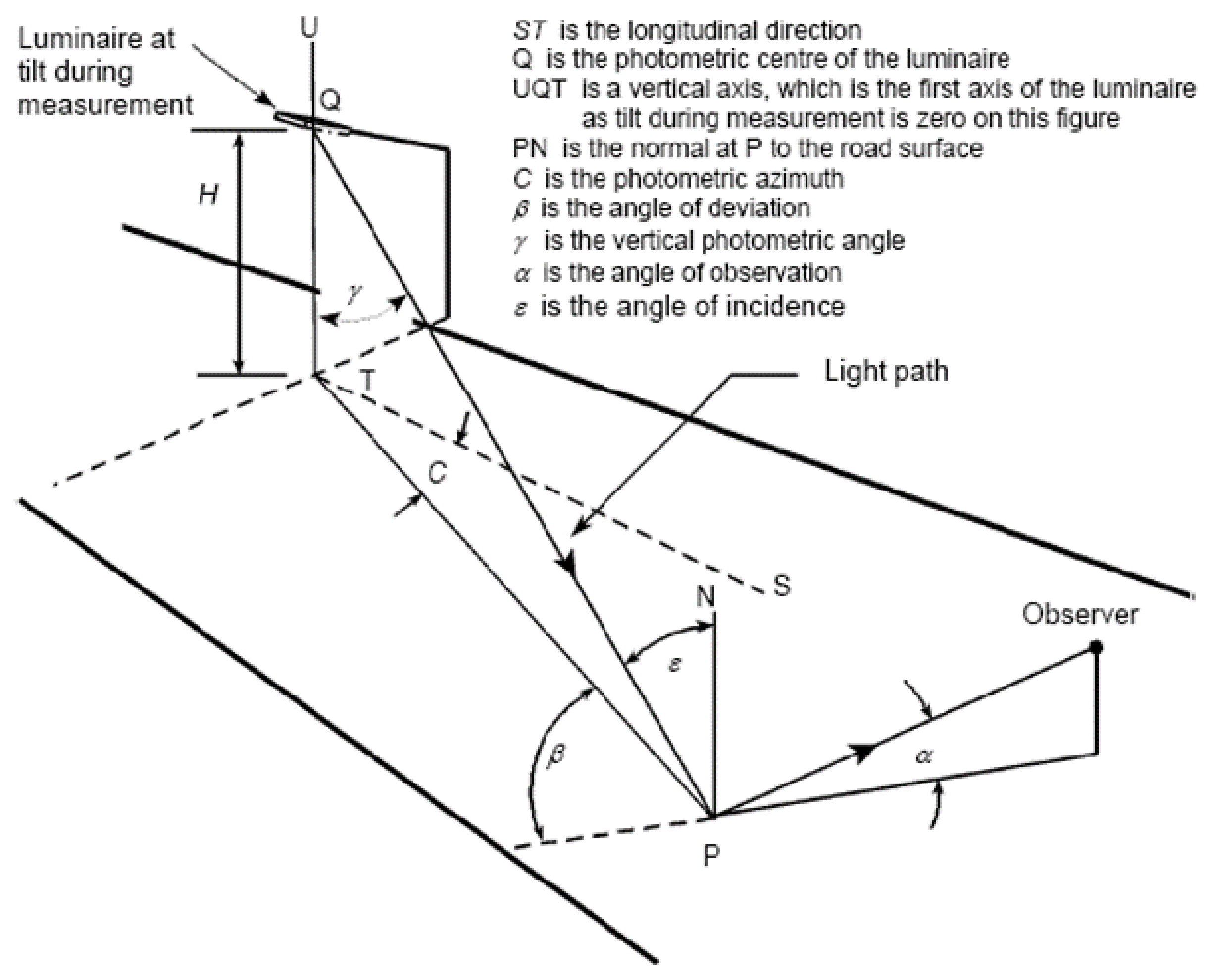
As shown in Figure 1, the relationship between users’ viewing angles and the angle of the road surface scattering characteristics is clearly defined in the CIE-140-2000 [30] measurement regulations. When calculating the level of luminance for the road surface, its brightness coefficient (r-table) should be taken into consideration. The reflection coefficients of incident light from different angles are non-identical. Even if the luminance is measured from the same observation point, different luminance levels will be generated due to the difference in the angle of the observation position. Therefore, when it comes to road surface, the luminance measurement is relatively more complicated than the illuminance measurement.
Recent years, the measurement methods for road lighting have made significant progress. Studies [31] have established a complete measurement system that can assess the luminance and illuminance of road images on continuing roads, which can be considered as a reliable method and of reference value when it comes to on-site road lighting testing and acceptance. Some researchers [32] have also combined the illuminance measurement system with vehicles so that the road surface illuminance level can automatically be recorded while in motion. Although the method is quite convenient, the interference factors, such as vehicle lights, would be hard to avoid during the whole measurement process. The designs of most of the measurement equipment are based on the theory of photonic vision. Since the roadway lighting at night is often in a mesopic-vision environment, the S/P ratio of the street light spectrum will greatly affect the measured value. This theory is typically suitable for road lighting that has a dark surrounding environment [33]. Pedestrian demands are one type of issue that has received attention in recent years. Besides considering the visual experience (clarity) of the driver, roadway lighting should also take into account the safety of the pedestrians. Researchers [34] used ILM to analyze the contrast of pedestrian, road surface and background luminance from the drivers’ fields of view, which are different from the traditional measurement design, which only evaluates the road surface illuminance of the crosswalk. Another study [35] introduced some practical measurement experience. Since the measured value of the luminance depends on the on-site road surface condition, the study points out that the road surface reflectivity and road curves are both influencing factors. Therefore, in addition to the lighting simulation software data, the theoretical basis should also take into consideration of the on-site road surface conditions for verification.
2. Materials and Methods
Before undergoing secondary optic design, it is necessary to evaluate LED energy to understand the luminous flux distribution state. The optical elements can transfer the existing energy of the light source to the target area forming an effective light intensity ratio that forms a presupposed photometric curve. This paper uses the concept of “zonal flux” to evaluate the proportion of luminous flux in each zone based on different light types so as to adjust effectively the angle of incident light and outgoing light; at the same time, “freeform surfaces” and “iterative calculations” are used to calculate the 3D structure of the optical components to figure out the correct curvature of each light zone.
2.1. Zonal Flux
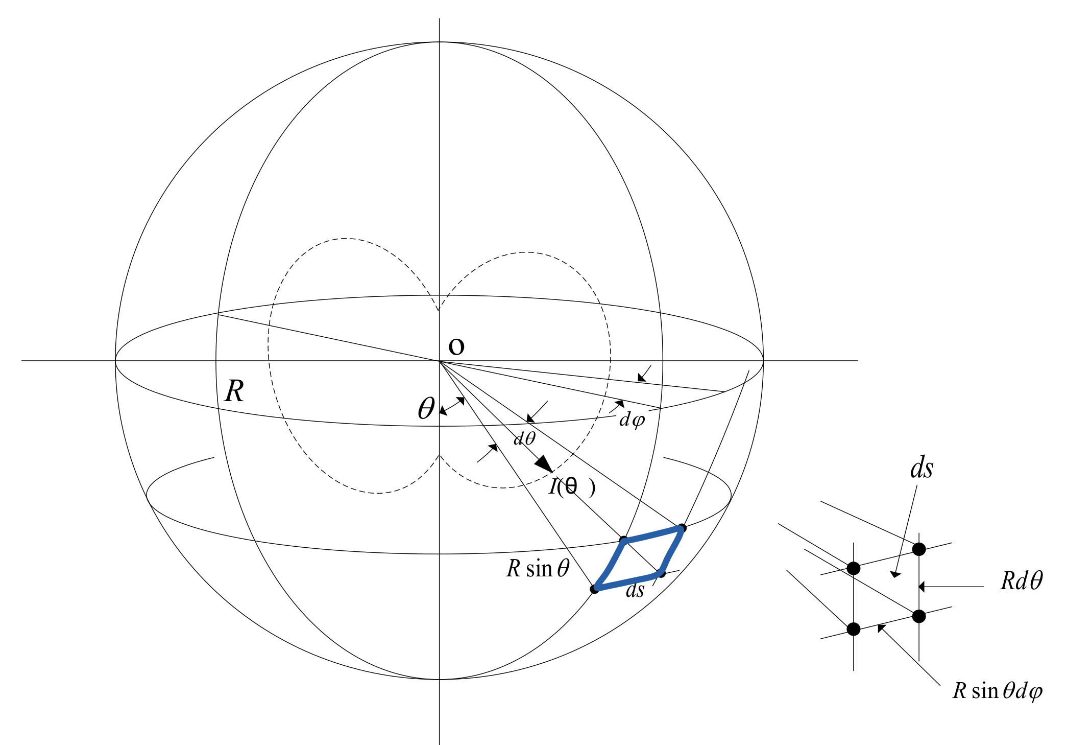
An imaginary spherical surface is used for calculating luminous flux, as shown in Figure 2, with point O as the center of the sphere and radius R. If luminous flux in a certain direction is required, it can be calculated by multiplying the luminous intensity with the solid angle from that particular direction. Therefore, when a certain direction is , light intensity is , spherical projection area is , solid angle is , luminous flux is and the total zonal flux of the sphere is , the equations are shown in Formula (1)–(4). If the beam pattern is display in a symmetrical light distribution condition, that is, , then the total zonal flux can be calculated by Formula (5) [36]:
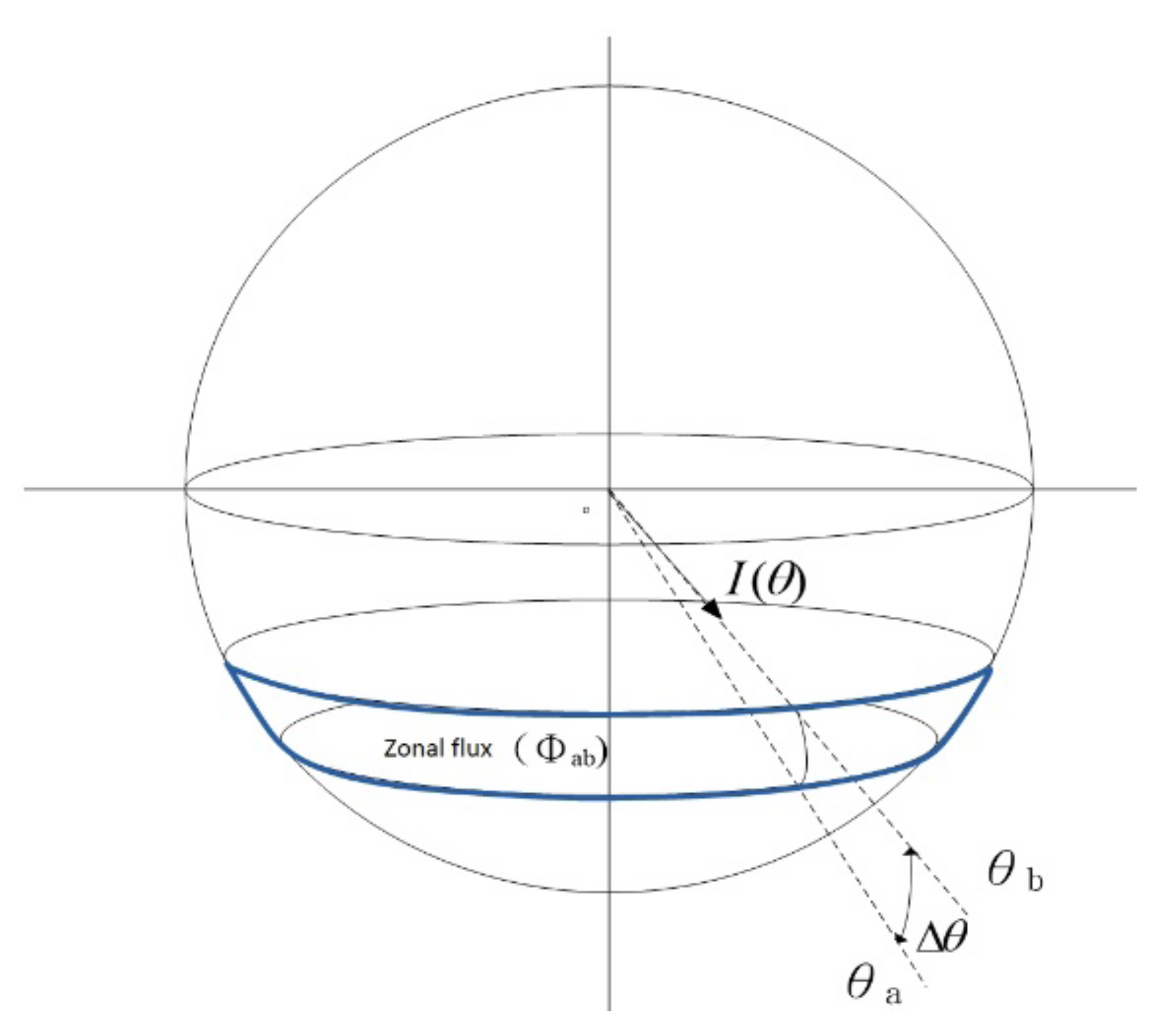
If the light source is distributed irregularly and cannot be expressed by a mathematical function, then, when calculating the total zonal flux, Formula (6) should be applied instead, where is used as the solid angle of Δ, which is also regarded as the ring coefficient. If the required solid angle Δ is between the vertical angle to of the light distribution, then the ring coefficient and the zonal flux can be obtained using Formula (7) and (8) as shown in Figure 3. Table 1 is a list of ring coefficients that correspond to angles less than 90° and are calculated at 10° intervals.
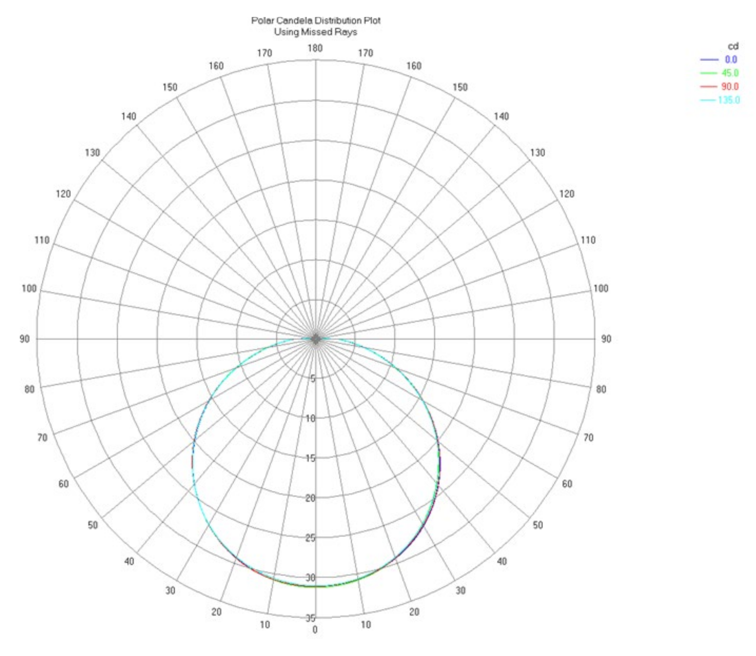
Figure 4 is a standard Lambertian LED light distribution and its total luminous flux is 100 lm. At intervals of 10°, we use the above zonal flux formula to obtain the luminous flux of each zone, as shown in Table 2. Moreover, the luminous flux for the whole circumference is confirmed with a total of 100 lm. As is evident, while the LED light source might have the highest central luminous intensity, the luminous flux is only about 3% within the vertical angle of 0°–10°. This means that high luminous intensity is not equivalent to high luminous flux. Since the secondary optical design uses luminous flux distribution to adjust the output beam angle, zonal flux analysis is of considerable importance for the light source and targeted beam pattern.
2.2. Freeform Surface
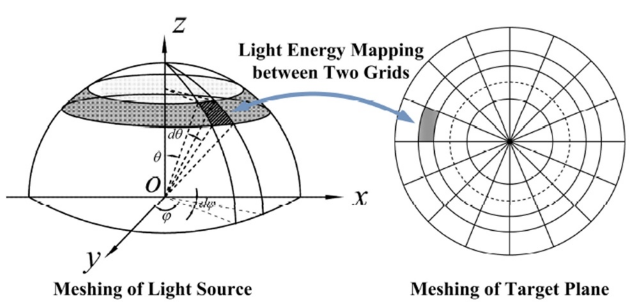
Freeform surface generally refers to an irregular or non-symmetric smooth surface, which varies from that of an ellipse, a parabola or conic curve formed with a specific shape. Freeform surface was mainly used in the design of the exterior structure of car bodies or ships in the early days. The application of optical design is mainly based on the relationship between light distribution and target illuminance, which is conformed to Snell’s law, Etendue conservation and the Edge-ray principle, etc. When a derivative formula of the curved surface is established then we can obtain the control points of the component structure and model the freeform surface. In this paper, the distribution of the LED light and the required light type of the observation surface are analyzed using zonal flux; the incident light source is divided into grids and correspond to the outgoing position of the target plane. Figure 5 is a display of the light energy mapping of the freeform surface.
When solving or optimizing freeform surfaces, a large number of complicated mathematical calculations of differential equations are commonly used. When it comes to basic geometric optics, the intersection of the linear equations, based on the incident light vector and the tangent vector, is the control point for the curve. The calculation process is relatively simple and could apply to most of the geometric curved surfaces. However, when the number of control points is insufficient, for instance, if we calculate at intervals of 5° or 10°, it may lead to deviation in the tangent vector [17]. Therefore, when designing, a large number of control points should be used to create a freeform surface structure to reduce errors although it will also increase the computing time during modeling. In addition, when it comes to different lens applications or output angle beam pattern, the reasonable number of control points demanded will primarily be based on related designing experience. While the goniometer measures luminaire distribution at intervals of 2.5°, the optical lens design in this paper calculates at intervals of 1° when analyzing, its deviation is less than 1% when compared with using intervals of 0.1° in horizontal plane analysis. Moreover, when calculated at intervals of 1°, the software efficiency is quite good and the control points of the freeform surface are very accurate.
2.3. Geometric Analysis of Optical Refraction Surface in Roadway Lighting
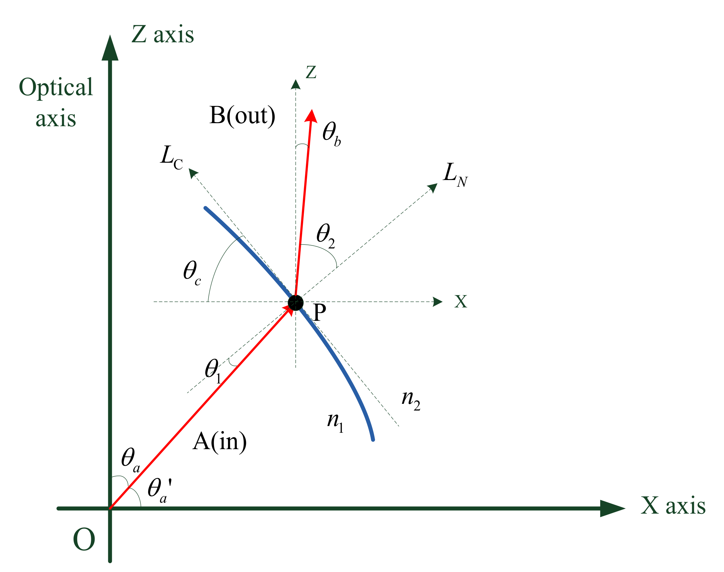
According to the law of refraction, which is generally known as Snell’s law, the optical axis Z is use as a reference for 0° as shown in Figure 6, the ideal light source O is refracted to direction B at from a certain incidence angle A which is . and are the incident light and the outgoing light from the normal line of point P, respectively. is the included angle between the normal line at point P and the horizontal line. Finally, we can obtain the slope of the tangent line at point P and the tangent line equation of the reflecting surface by the mathematical relationships as follows:
The relationship between the tangent line at point P and the horizontal line angle is as follows:
Based on Snell’s law, the relation of and is as shown in Formula (8). This study uses PMMA and PC for lens design, and the refractive index of medium is 1.49 and 1.59 respectively; the second medium is air, whose refractive index is 1. Formula (6) is inserted into Formula (7) to obtain the complete relation:
After dividing Formula (8) by , we obtain Formula (9) and substitute it into Formula (7) to obtain angle , which is the angle between the tangent line at point P and horizontal line as shown in Formula (10):
We can obtain the slope of the tangent line at point P from Formula (10).
The tangent equation at point P can be obtained from Formula (11).
2.4. Establish the Freeform Surface Formula for a Roadway Lighting Lens
The ways of emitting light for a roadway lighting lens are different from that of a total internal reflection lens and, due to its larger irradiated surface, a wider emergent angle is usually required. Generally, the incident light will be refracted twice to meet the demand distribution. In this study, we divided the road lighting lens components into a central refraction lens area and freeform surface refraction area. The mathematical model for each curve surface is as follows.
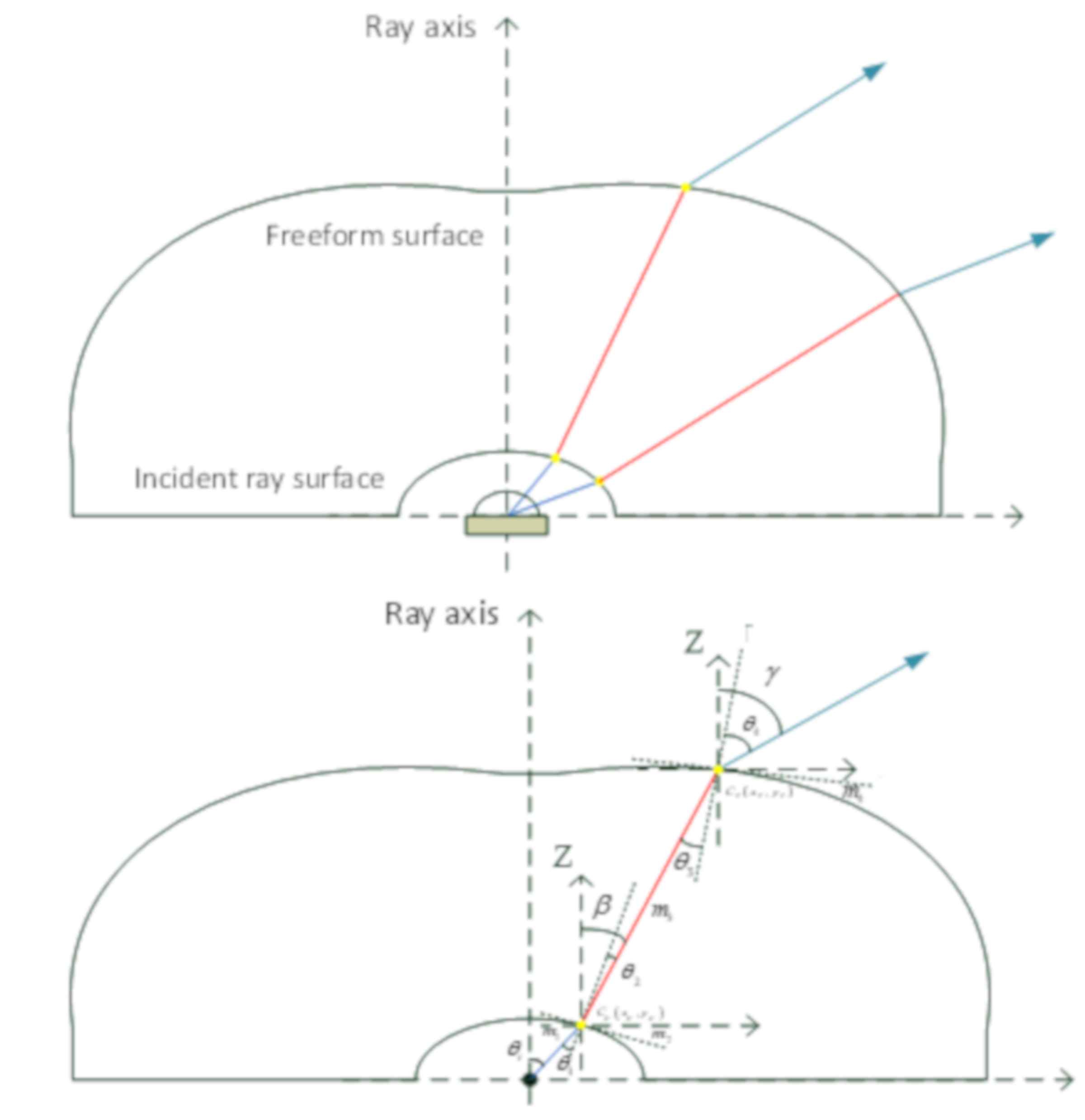
There are two main surfaces, which include the incident ray surface (first refraction) and the freeform surface (second refraction). The coordinate of the incident ray is with incident angle and refracting angle , which is also the incident angle of the freeform surface at coordinate . After the second refraction by the curved surface with m4 slope, the final refracting angle is .
2.4.1. Incident Ray Surface
After the LED light enters the lens, it travels according to the rule of refraction. Since the incident surface is a freeform surface, as shown in Figure 7, the location of each point will be obtained through calculations. The calculation is roughly the same as that of a total internal reflection lens regarding the central refractive lens. First, we need to build the linear equation of the incident light:
where is the incident angle of the LED light and is the slope of the LED incident light.
The relation between the incident lens and the geometric relation of and is shown in Figure 7 and is based on Snell’s law, with . After the light passes through the freeform surface, is the included angle between the light and the optical axis, the calculation formula is as shown in Formula (14):
Regarding the freeform surface control point of the intermediate lens, the tangent equation and the slope equation passing through the control point are as follows:
We solve the simultaneous equations of (13) and (15) by using an iterative method to obtain the coordinates of the control points of the central refractive lens area and connect the points to form the curved surface of the lens.
2.4.2. Freeform Surface Refractive Lens Area
After the LED light is refracted into the lens through the incident ray’s surface, it travels according to its optical path and increases its output angle after travelling through the freeform surface refraction lens area. The coordinates of each are obtained after calculation. The light travels through the incident lens area and passes the point. The ray equation and slope relationship after refraction are as follows:
Based on Snell’s law, when discussing the geometric relation of and in Figure 7, where is the included angle between ray axis and refracting ray from freeform surface, the calculation formula of is as shown in (22):
In addition, we establish the tangent equation of the light that travels through the freeform surface and that passes point as in (23). The tangent slope of the freeform surface , as shown in (24), is obtained by using characteristics of refraction.
We solve the simultaneous equations of (19) and (23) by using an iterative method to obtain the coordinates of the control points of the freeform surface refractive lens area, and the points are connected to form the curved surface of the lens:
2.5. Secondary Optical Design of a Roadway Lighting Lens
This article has designed the optical lenses separately according to two road lighting requirements, which are “equal illuminance” and “equal luminance”, and mainly discusses the energy distribution of the transverse roadway lines (TRL). The photometric curve of the lighting distribution is mainly Type II-Medium.
2.5.1. The Applied LED Light Source
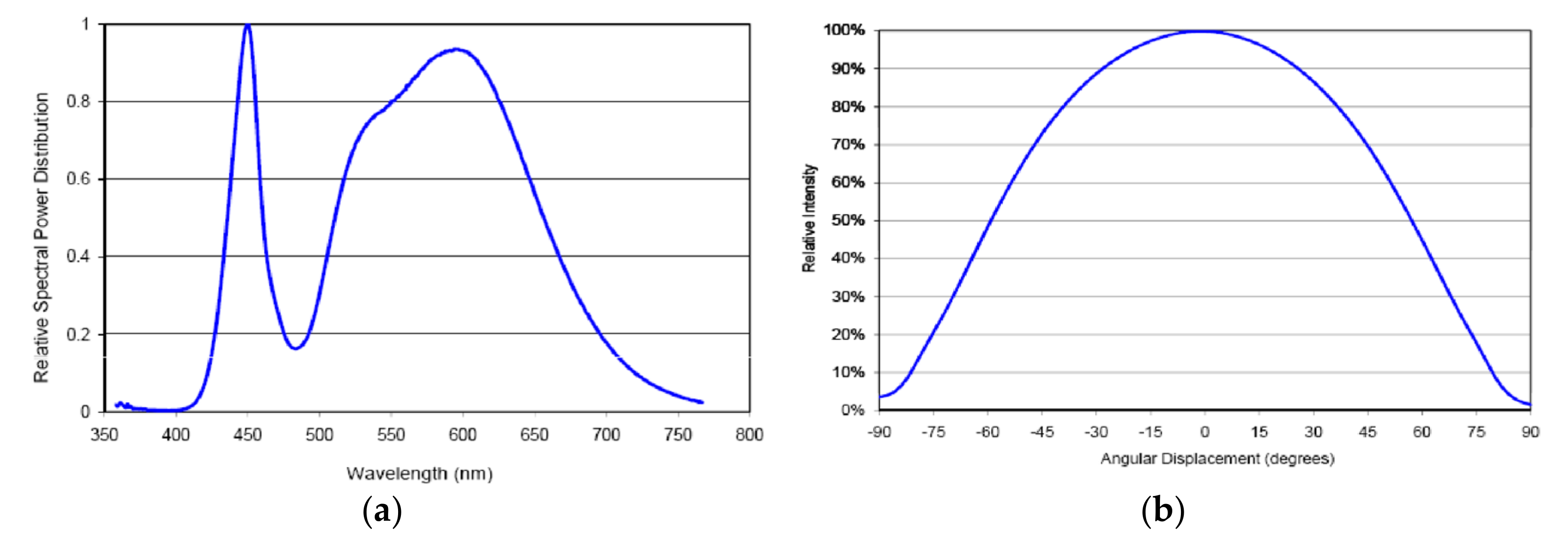
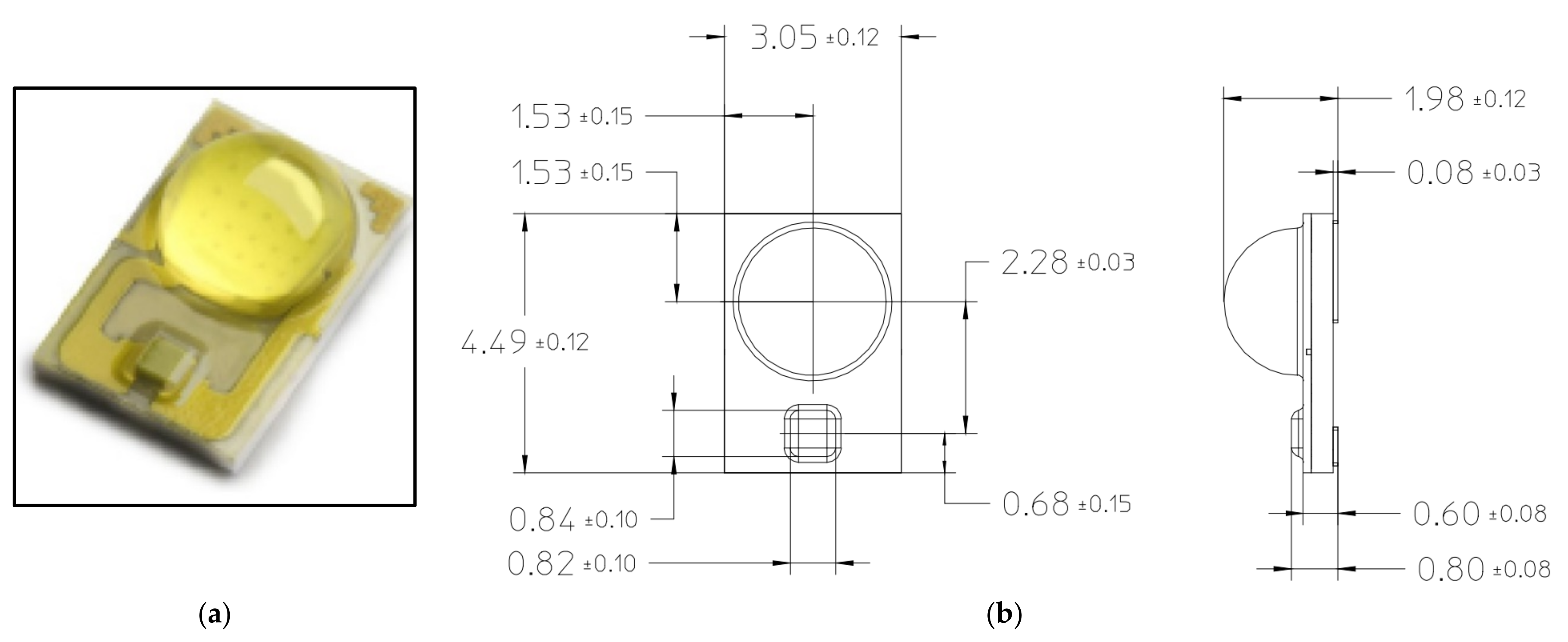
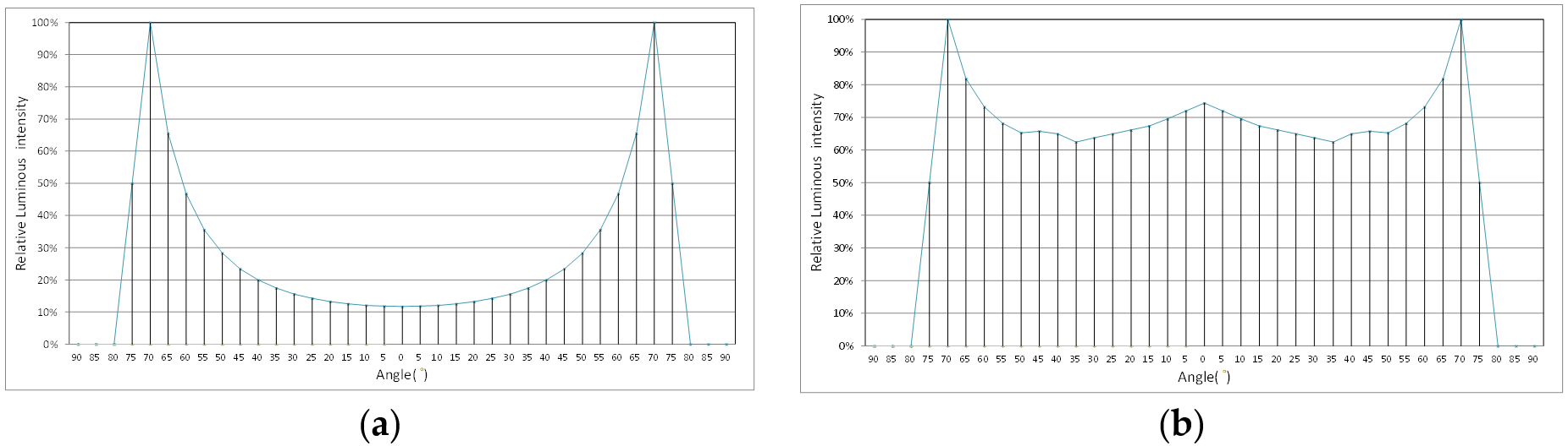
Lumileds LUXEON Rebel ES LED [37] was used as the light source for the design of the roadway lighting lens. The photoelectric specifications are shown in Table 3. This study uses 4000 K color temperature and a color rendering index (CRI) of 85. Its effective beam angle is 120°. The spectral power distribution and relative intensity versus angular displacement are shown in Figure 8. The entity diagram and mechanical dimensions are shown in Figure 9.
2.5.2. Lens Design of Roadway Lighting
We design two kinds of lenses based on the R3 road surface (dry) and W1 road surface (wet) and will rename the lenses to Type A and Type B respectively. Type A lenses are designed for the purpose of equivalent road illuminance on R3 roads, so the photometric curve will be similar to the batwing model. Type B lenses are designed for the purpose of equivalent road luminance especially on W1 roads to maintain good uniformity on rainy days and to avoid the zebra effect.
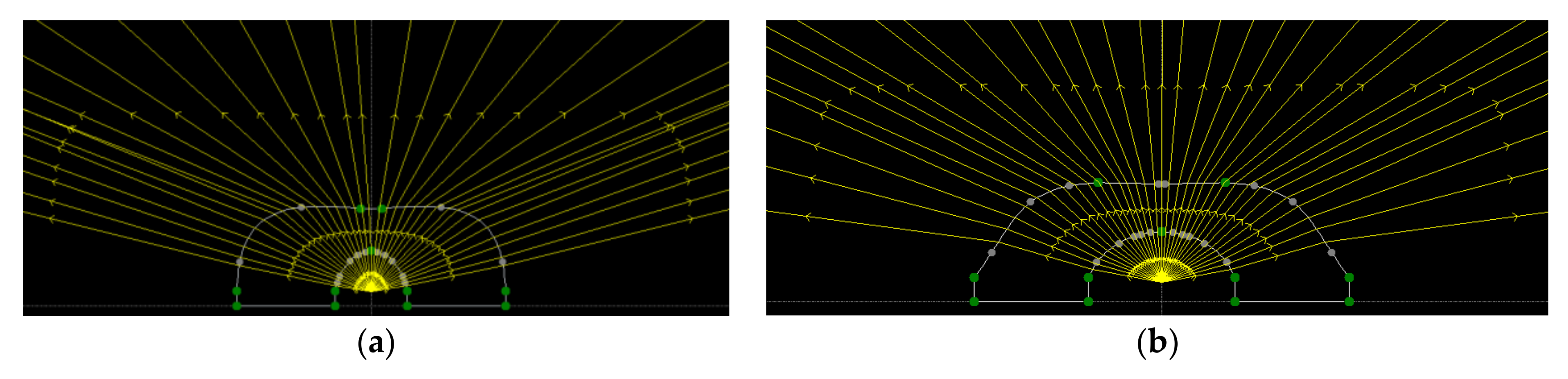
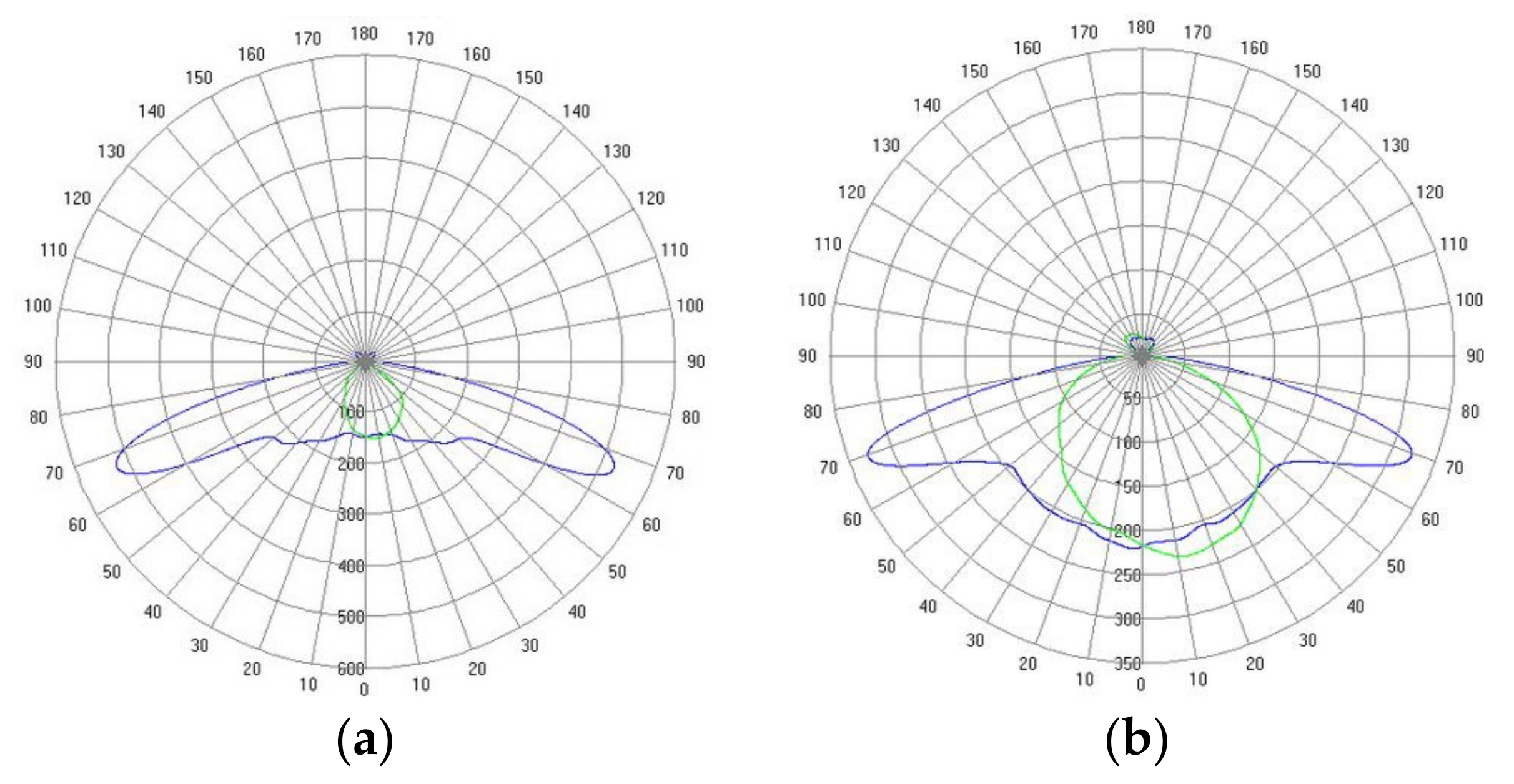
Roadway lighting has a wider light output angle and is more likely to have glare issues. Therefore, when defining the targeted beam pattern, it is very crucial to pay close attention to the maximum light output angle and half intensity beam angle. The lens in this article is designed using PC material. Figure 10 displays the targeted beam pattern according to the two lighting requirements of a roadway lighting lens, and zonal flux is used for analysis. The estimated correlation between the incident light and the outgoing light based on the luminous flux ratio of each angle is shown in Table 5. All the light needs to do for a large angle of energy transfer and the light path of the lens is shown in Figure 11. Figure 12 displays the uniform illuminance and uniform luminance photometric curve of the final (lens) design.
3. Results
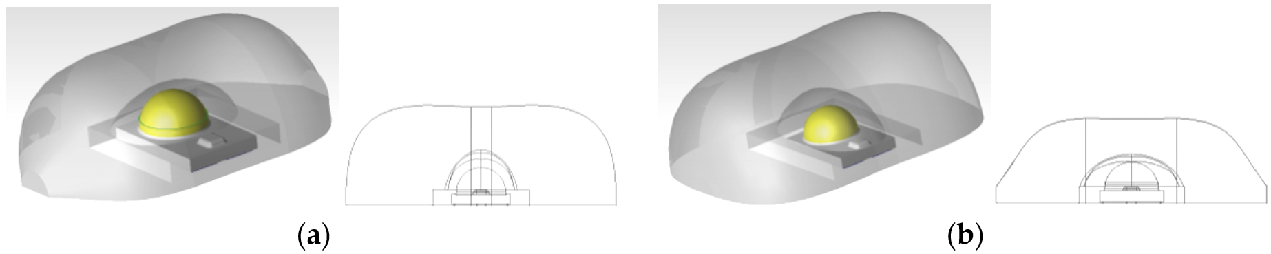
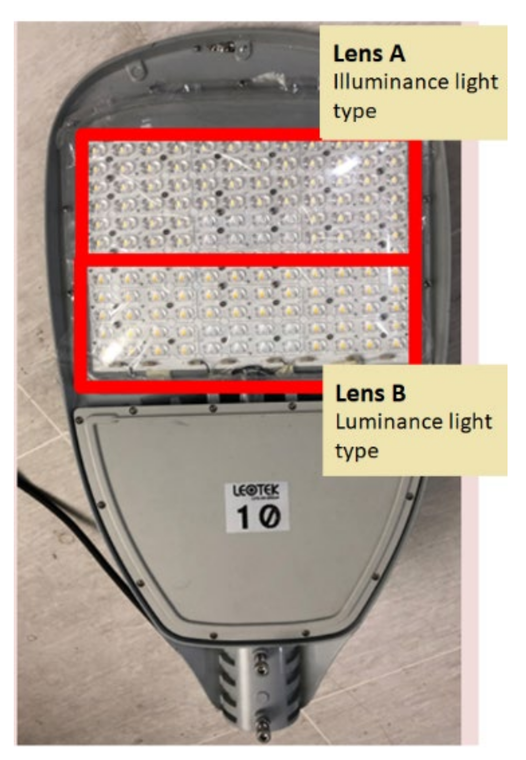
The optical design is based on the above-mentioned zonal flux theory. Figure 13 displays the structure of the Type A and Type B roadway lighting lenses. Figure 14 is the actual productions of the two lenses, which are assembled into the same roadway lighting device, equipped with an intelligent lighting control system. In addition, an imaging luminance meter is used for roadway lighting calculations, with a wider range of sensing and an intelligent light control system that are used to build an adaptive roadway lighting control strategic system, which aims to achieve efficient human-centric lighting. The imaging luminance meter is used to calculate the value and uniformity of luminance, whether it is a dry or slippery roadway. The feedback signal is used to control the smart system, which will adjust and output optimal photometric light curves accordingly.
3.1. An Overview of the Human-Centric Intelligent Roadway Lighting Syterm
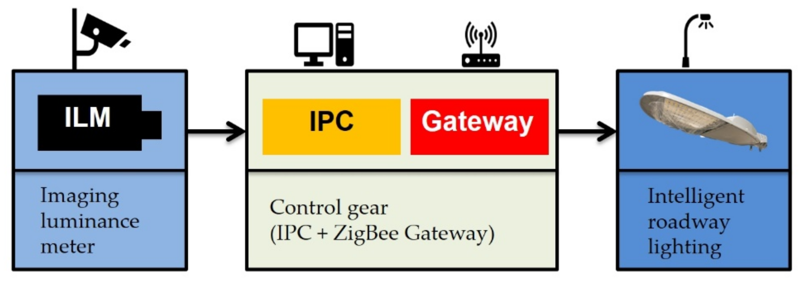
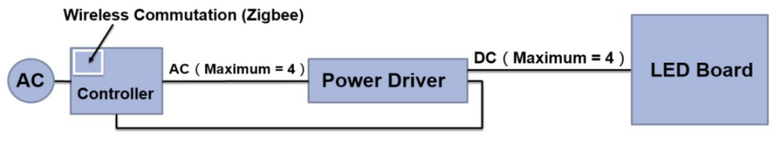
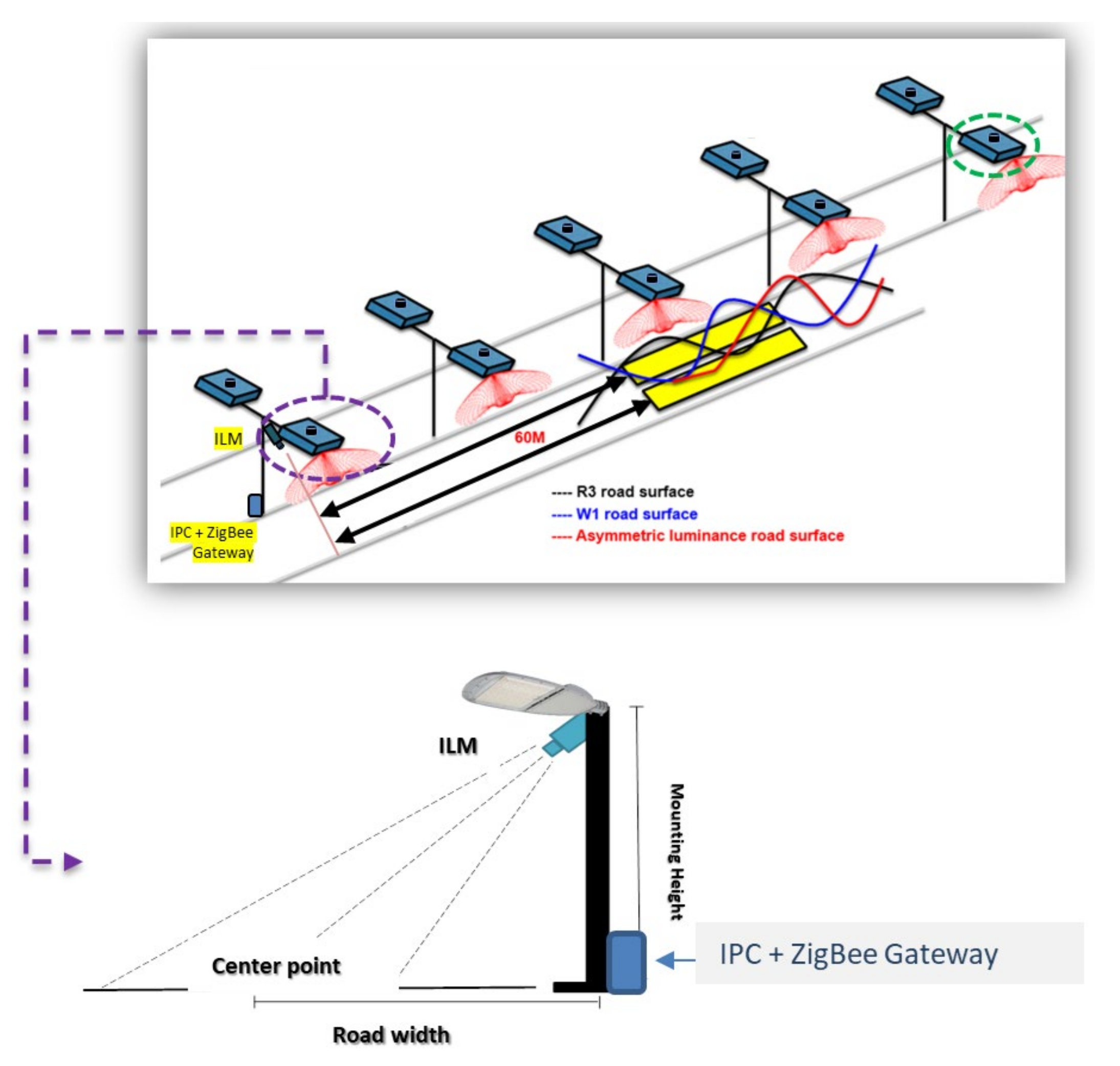
The LED human-centric intelligent roadway lighting system includes three units: a roadway image luminance recognition technology, an intelligent lighting control interface and a human-centric LED roadway light. The framework is shown in Figure 15. The image luminance meter detects the roadway luminance and returns the signal to the control system IPC host for analysis. After the signal is calculated by the control logic of the system algorithm, the command is then transmitted to the roadway lighting power supply through the wireless communication protocol ZigBee, which will output the optimal photometric light curve that meets the driver’s needs. In order to operate smoothly with the lighting control module, as shown in Figure 16, the luminaire is designed with two lens that are combined and adjusted by the partitioned power switch. In addition, wireless control module ZigBee is used for signal control, which allows the system to be divided into multiple groups of control signals in switching the output. There are multiple groups of customizable channels with different lenses and light panels to meet the demands for various light types and illuminances. Figure 17 is a schematic diagram of the system setup. The intelligent roadway lighting control experiment on site is shown in Figure 18.
3.2. The Operation of the Human-Centric Intelligent Roadway Lighting System
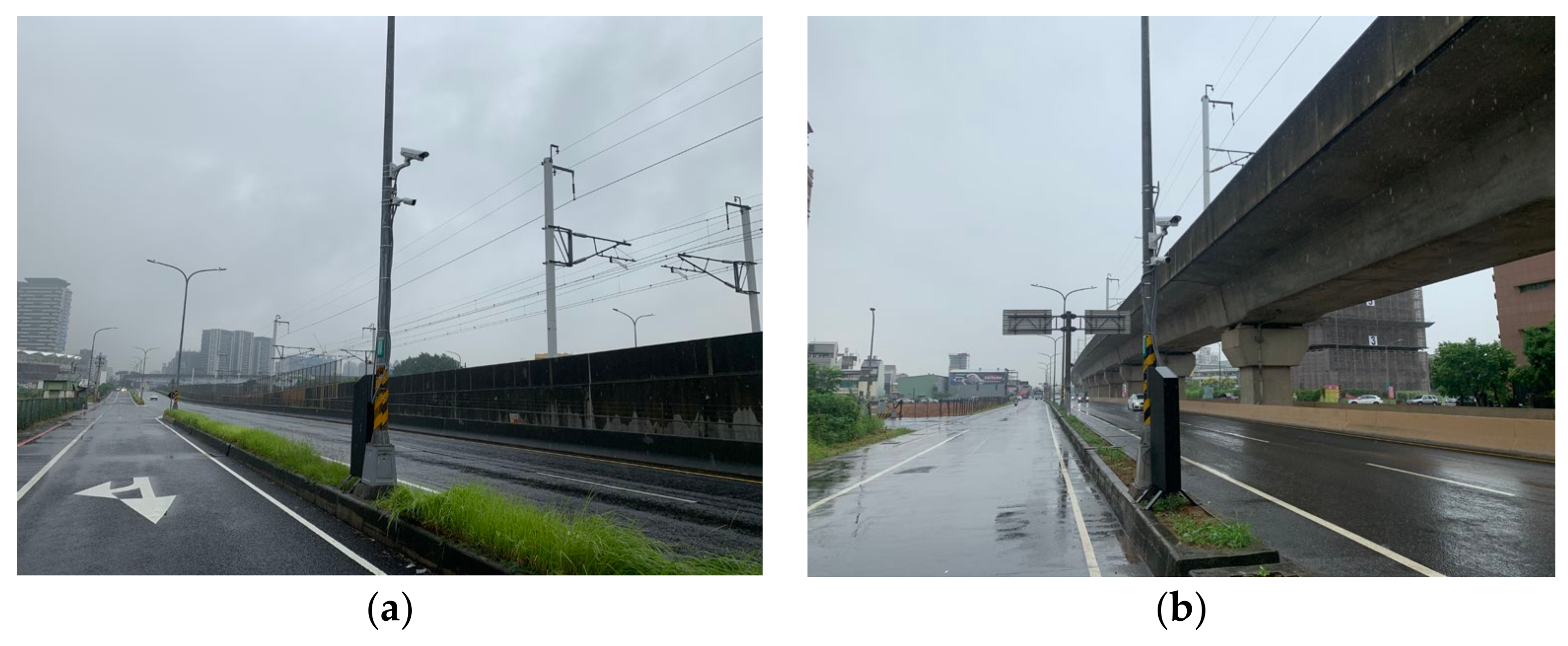
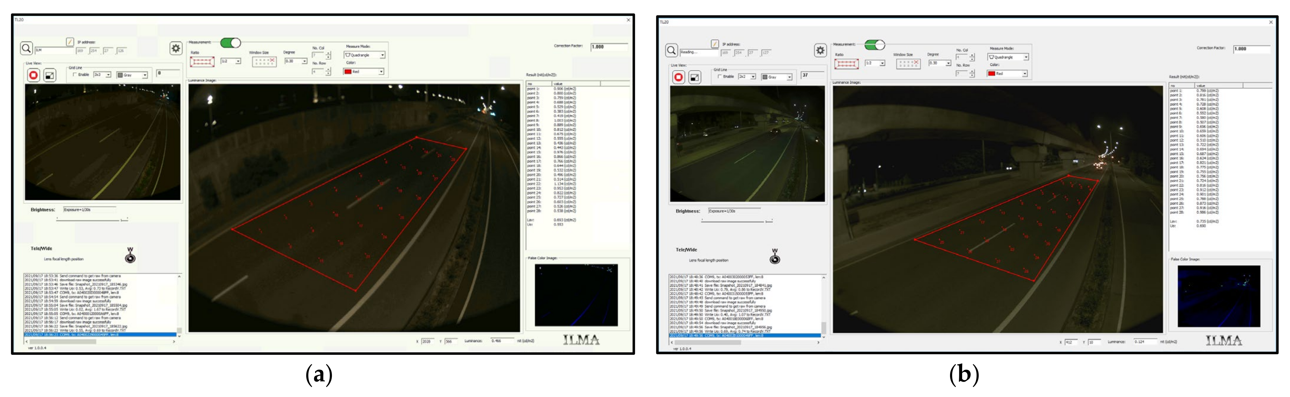
This study selected a total of two roadways at Taoyuan City in Taiwan for the actual human-centric intelligent roadway lighting system test. Each area was expected to install 24 LED street lights. In this article, each imaging luminance meter is used to control 12 lamps and was installed on a street lamp pole. The pole was also equipped with a control system. The actual installation status on site is shown in Figure 18. Figure 19 shows the imaging luminance meter observation results of the two test sites. The observation range and sampling points can be adjusted according to the road type or the relative position of the imaging luminance meter installed. The sampling frequency set by the system reads the roadway luminance value once per minute to calculate the average luminance and luminance uniformity of the tested area, which will then be used as a reference for adjusting the light output of the human-centric intelligent roadway lighting.
The software presented in Figure 19 is the analysis software of ILM named ILMA, which could set the measurement range, points, spacing and shutters, etc. ILMA is capable of saving records, including real-time images, average luminance and luminance uniformity (UO, UL) per minute, or on other time schedules, while also automatically ignoring the motion of the vehicle to avoid getting the wrong calculation and data.
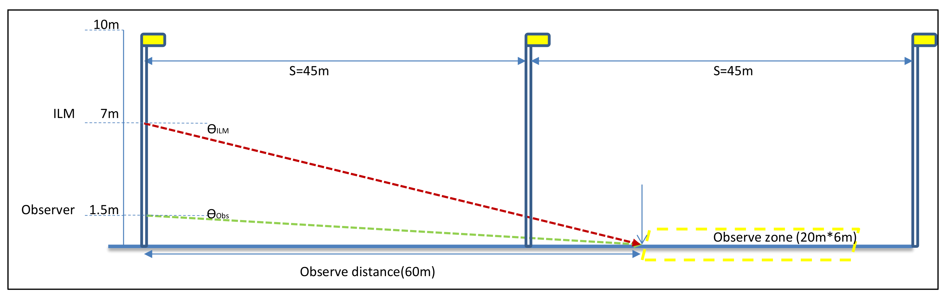
This article refers to CIE 140 (road lighting calculations), which suggests the distance and height of the observer are 60 m and 1.5 m respectively. However, based on the actual scenario at Taoyuan, Taiwan, the spacing of the installations were 45 m apart and the mounting height of the roadway lighting was 10 m. Therefore, we installed ILMs on the lighting pole, with a tilt angle () of 6.65°, which were 60m from the “observe zone” and 7 m in height, as shown in Figure 20, to reduce the influence of the rush hour traffic.
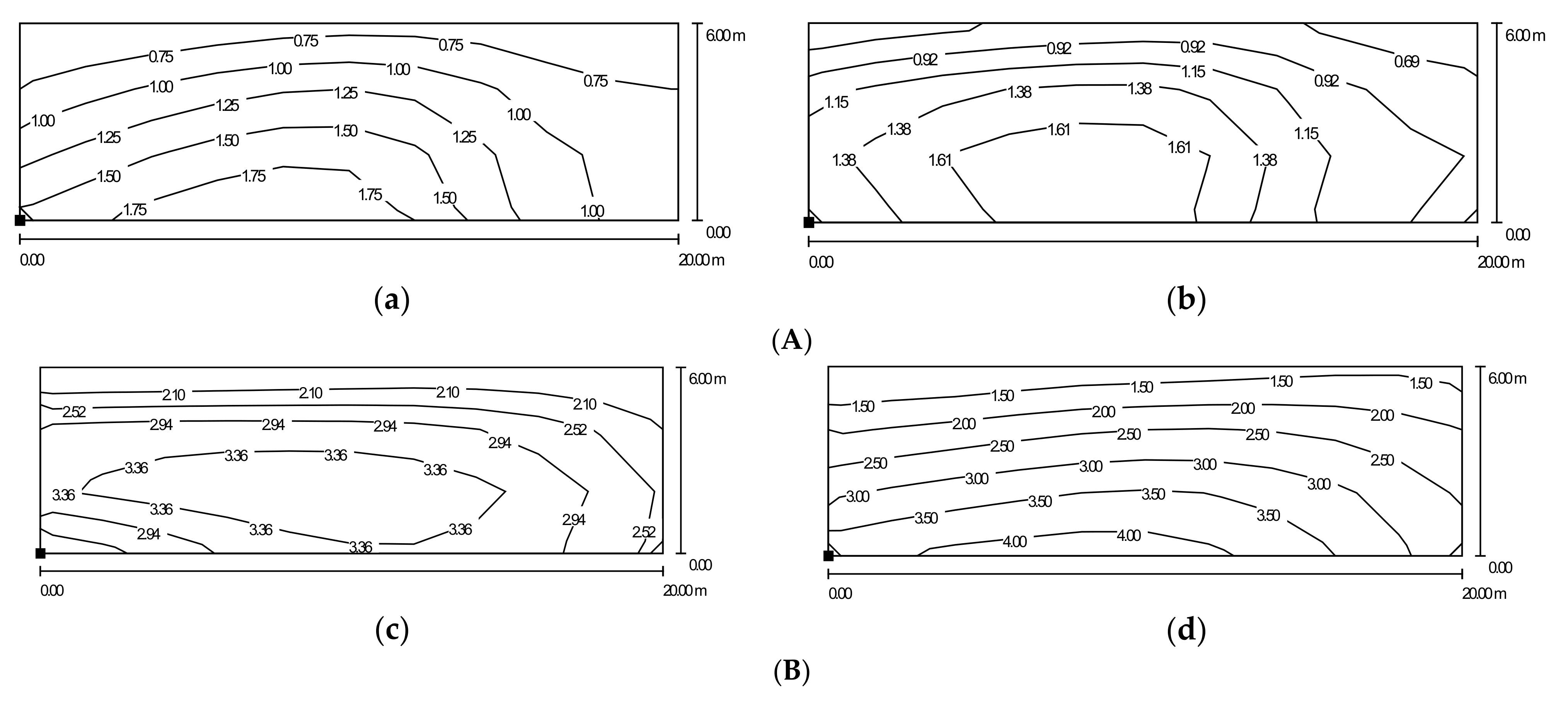
As the road surface conditions could not be the same everywhere, and the roads in our scenario are not newly built surfaces, we used DIALux software to simulate the relationship of the ILM and the observer to avoid external disturbance. Figure 21A,B are the simulation of the luminance contour map of the Type A lens on the R3 road surface and the Type B lens on the W1 road surface. Table 6(A) shows the DIALux simulation results between the ILM and the observer on the R3 and W1 road surfaces, this table shows that the Type A lens has better illuminance uniformity but is unqualified for luminance uniformity, especially on the W1 wet road surface. In contrast to the Type A lens, the Type B lens has good illuminance uniformity and also provides excellent luminance uniformity on the R3 and W1 road surfaces. Table 6(B) is the ratio of the ILM and observer regarding Type A and Type B lenses. Lastly, we use the average ratio to compensate the ILM measurement result when calculating the real luminance from the observer. When compared with Table 7, we discover that the average luminance is different from Table 6(A) due to the actual status of the road surface, or for other reasons. The simulation results are still helpful and could be taken as a reference for optical design on the ideal road surface, especially in luminance uniformity to contribute to the early prevention of the zebra effect on any kind of road surface.
3.3. The Benefits of the Human-Centric Intelligent Roadway Lighting System
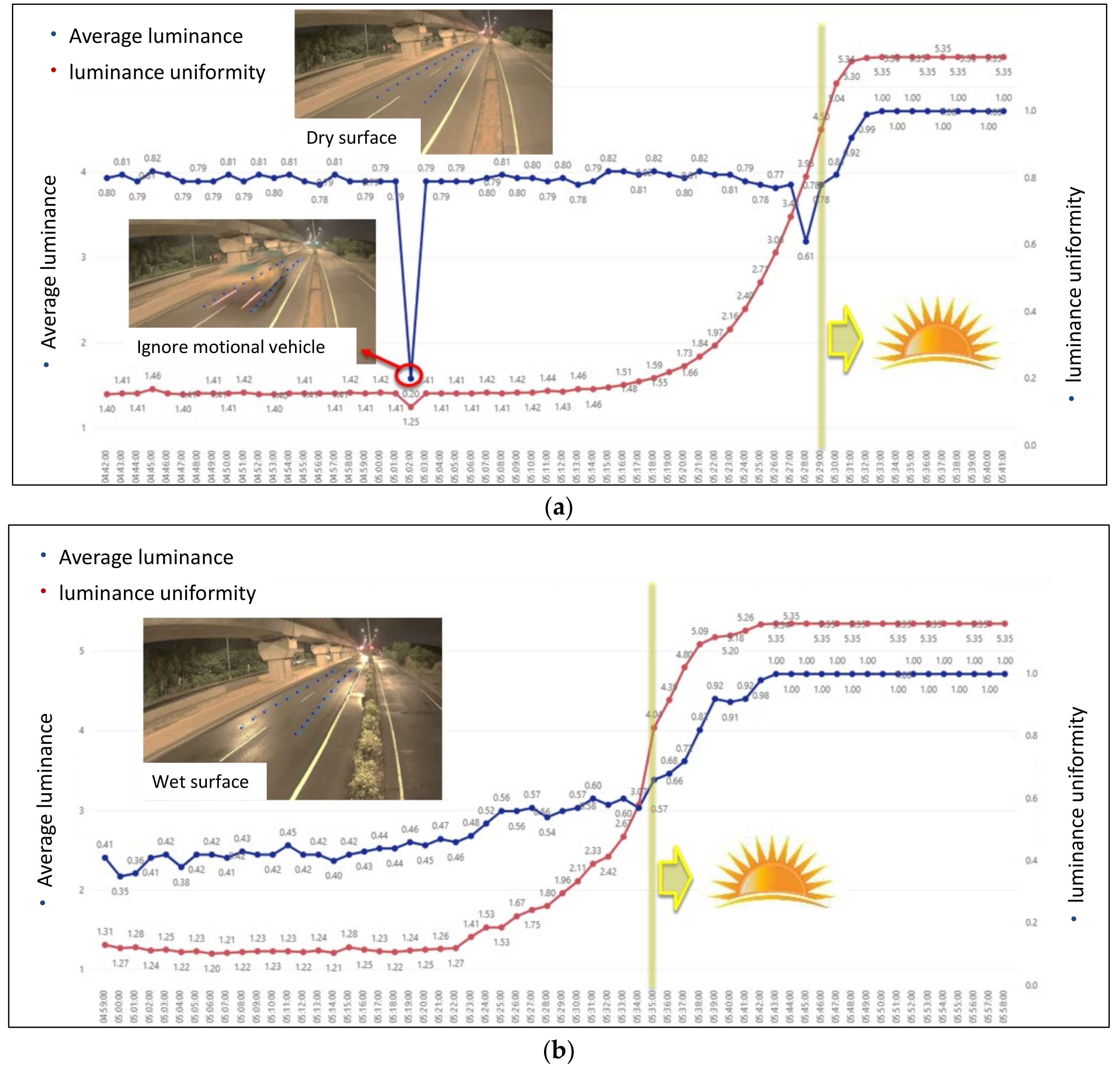
After a long-term observation using the imaging luminance meters, we have established a roadway lighting adaptation model. Figure 22 compares the lighting conditions for when the road is wet and dry. The level of luminance value is shown in Table 7. The average luminance of the wet road is around 8.5–12%, which is lower than that of the dry road, and the luminance uniformity drops below 0.5. Therefore, according to the data obtained, we can use this to set up control logic of the output of the street light type. When the system considers the road condition to be wet and slippery, it will switch to the uniform luminance light distribution, if the road surface is dry it will switch to a uniform illuminance light distribution.
According to the records of road luminance uniformity by the ILM from September, we collected the highest and lowest value per day from 19:00–04:00. The standard deviations are shown in Table 8:
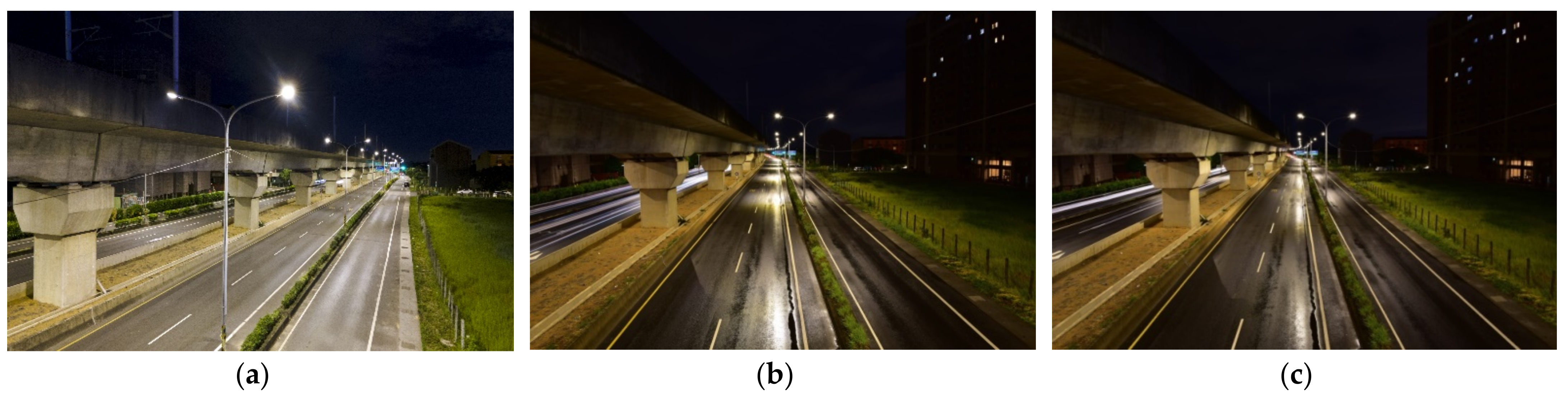
Taking Section 5 of Gaotie South Road as an example, from left to right, Figure 23 shows Type A distribution on dry roads, Type A distribution on wet roads and Type B distribution on wet roads. From what we can tell, the Type A distribution shows good uniformity on dry roads. When applied to wet roads, the change in road surface reflectance produces a strong contrast (causing the zebra effect). However, if the light is switched to the Type B distribution it can provide drivers with a relatively safer and more comfortable driving experience where they are able to see the road surface more clearly. Therefore, the intelligent roadway lighting system proposed in this paper used an imaging luminance meter to detect the roadway lighting status and automatically switch and adjust to the optimal output of light distribution to achieve the best road lighting conditions. The main focus of our research is decreasing the zebra effect; due to the road luminance factor q0 (related to the overall reflectance of the pavement) it is different for each roadway surface. Before designing the secondary optical lens for roadway lighting, it is important to define which kind of road surface is our target. In this case, we chose wet road surface (W1) as our design target, and one of our two lenses named Type B (uniform luminance) achieved the target of uniform luminance for improving the zebra effect on wet roads.
4. Discussion
The engineering design requirements of roadway lighting usually take both the road surface illuminance and the luminance conditions into consideration. Among them, road surface luminance is highly related to the visual experience of the road users. Hence, road surface luminance performance has been regulated around the world as an important evaluation index. Since the luminance value is inseparable from the reflection characteristics of the pavement material, if the scattering characteristics of the road surface change it would also cause a significant visual difference. Hence, the luminance value of the roadway lighting should be adjusted according to the road conditions. For example, the reflectivity of wet and slippery roads in rainy days is higher than that of dry roads where uneven reflection spots on the road are likely to cause indirect glare or poor uniformity, which contribute to the degrees of risk while driving.
Traditional roadway lighting optics are all designed with fixed light distribution. Usually, the road surface material is preset to R3 pavement characteristics as the standard parameter when evaluating the luminance distribution. Therefore, it is relatively difficult for traditional lighting to adapt to various environmental conditions. In situations where the weather or road surface conditions change abruptly, drivers will be exposed to poor lighting quality since the uniformity of the light distribution is usually designed for standard road surface conditions. Hence, when it comes to bad road conditions, the visual uniformity will drop drastically also. This paper proposes a LED human-centric roadway lighting system that can adapt to different road conditions, hoping to provide drivers with a safer road environment at all times.
In this paper, an imaging luminance meter (ILM) is used for detecting and monitoring the luminance uniformity of road lighting. During 2007, due to the increasing awareness for energy saving and safety, one study [38] used an ILM to measure and analyze the luminance level of different kinds of road surface and of intelligent street lighting. In that particular article, measurement results of different road surface conditions including dry, wet and snow-covered roads are proposed. The results show that the luminance of the snow-covered roads is significantly higher than that of dry and wet roads. In addition, dry roads and snow-covered surfaces are less susceptible to height and distance when measuring and the standard deviation of luminance is around 0.03 and 0.02 respectively. While the measurement result of the wet road is much more susceptible to the observation point, which leads to a different measurement value. Therefore, when comparing the luminance level measured from the driver’s position with the installation point of the ILM, the luminance values of dry roads are relatively close while the luminance level of wet roads can reach a difference of more than 10%, which is close to the results of this paper. However, they did not mention the road pavement materials in their study. In our paper, we have stated clearly that we have used the R3 dry road surface and the W1 wet road surface for optical design and luminance measurement, so as to solve the zebra effect by improving the longitudinal uniformity of the road surface. Moreover, the adaptive roadway lighting system we established is able to monitor the road surface condition when it is affected by the weather in real time, through the ILM, and automatically switch to the most suitable type of lens to maintain high uniformity and ensure the safety of road users.
This research integrated many kinds of technology, from optical design to smart lighting control, to contribute and establish a lighting uniformity on the road surface. This is also the first project that imports an ILM system to roadway lighting in Taiwan. The project prior to this research focused more on energy saving, auto failure report, fast maintenance, etc., but this study focused on drivers’/road users’ safety, especially when it comes to driving on wet or slippery roads. Therefore, we designed LED fixtures with two types of photometric distribution, which are able to adapt to various road surface types, and used an ILM for sensing the lighting uniformity status on the road surface, enabling it to switch to the most suitable types of optic lenses accordingly.
The next step of this HCL LED system will be discussing the dimming strategy; due to maintenance issues, when undergoing the lighting design step, a higher level of illuminance and luminance at the initial step is applied in practice. Therefore, we need to further study the suitable dimming level based on the roadway lighting standard. This paper aims to propose a systematic method that makes roadway lighting intelligent by integrating an ILM device, which will hopefully garner and ensure the safety of the drivers.
5. Conclusions
This article proposes a design and control strategy for LED human-centric intelligent roadway lighting. First, it is based on the theoretical analysis of zonal flux. A simple and fast secondary optical design method for LED roadway lighting was established, aiming to achieve both road illuminance uniformity and luminance uniformity of the photometric light curve as the design goal. Thus, two types of optical lenses were produced and assembled to a street lamp to meet various lighting needs. In addition, they were equipped with an imaging luminance meter to detect the luminance level of the road in real time. Then, the return signal was used to adjust the output of the street lamp in a timely manner through the ZigBee wireless transmission control interface to meet the lighting demands, whether the road was wet or dry road. Then, a roadway lighting evaluation in practice was carried out where we found out that the lens designed for luminance uniformity did indeed provide quality road lighting, giving drivers a safer and more comfortable road environment.
Another future application of this research is for an autonomous car in the future. Taoyuan City in Taiwan has always aimed to be an advanced smart city and a demonstration field for an autonomous car. However, non-uniform luminance will cause not only the zebra effect but also unclear road markings. An autonomous car will configure the path of travel using camera images to check road markings. Based on the result of this research, we can now lower the chances of the zebra effect on the dry and wet road surface by using an ILM to automatically sense and switch optic lenses. With the novelty of this article’s findings, we can collaborate and integrate it with the future autonomous car system, which combines luminance sensing with imaging recognition by using an advanced ILM device.
Author Contributions
Conceptualization, C.-H.L.; methodology, C.-H.L., C.-Y.H. and K.-Y.L.; software, C.-H.L. and K.-Y.L.; validation, K.-Y.L. and S.-F.Y.; formal analysis, C.-H.L., K.-Y.L. and C.H.C.; investigation, C.-H.L., K.-Y.L., S.-F.Y. and M.C.H.; resources, C.-H.L., C.H.C. and S.-F.Y.; data curation, C.-H.L., C.-Y.H. and K.-Y.L.; writing—original draft preparation, C.-H.L., C.-Y.H. and K.-Y.L.; writing—review and editing, C.-H.L., C.-Y.H., J.-C.G. and M.C.H.; visualization, C.-H.L., K.-Y.L. and S.-F.Y.; supervision, C.-H.L.; project administration, S.-F.Y., C.H.C. and M.C.H. All authors have read and agreed to the published version of the manuscript.
Funding
This research received no external funding.
Institutional Review Board Statement
Not applicable.
Informed Consent Statement
Not applicable.
Data Availability Statement
All data generated or analyzed to support the findings of the present study are included this article. The raw data can be obtained from the authors, upon reasonable request.
Conflicts of Interest
The authors declare no conflict of interest.
References
- Alan, M. Solid state lighting—A world of expanding opportunities at LED 2002. III-Vs Rev. 2003, 16, 30–33. [Google Scholar]
- Brodrick, J. Next-generation lighting initiative at the U.S. department of energy catalyzing science into the marketplace. IEEE J. Disp. Technol. 2007, 3, 91–97. [Google Scholar] [CrossRef]
- Liu, M.; Rong, B.; Salemink, H.W. Evaluation of LED application in general lighting. Opt. Eng. 2007, 46, 074002. [Google Scholar]
- U.S. Department of Energy. Illuminating the Challenges Solidstate Lighting Program Planning Workshop Report; U.S. Department of Energy: Washington, DC, USA, 2003.
- Sun, C.C.; Chien, W.T.; Moreno, I.; Hsieh, C.C.; Lo, Y.C. Analysis of the far-field region of LEDs. Opt. Express 2009, 17, 13918–13927. [Google Scholar] [CrossRef] [PubMed]
- Yang, H.; Bergmans, J.W.M.; Schenk, T.C.W.; Linnartz, J.P.M.G.; Rietman, R. Uniform Illumination Rendering Using an Array of LEDs: A Signal Processing Perspective. IEEE Trans. Signal Process. 2009, 57, 1044–1057. [Google Scholar] [CrossRef] [Green Version]
- Moreno, I.; Avendaño-Alejo, M.; Tzonchev, R.I. Designing light-emitting diode arrays for uniform near field irradiance. Appl. Opt. 2006, 45, 2265–2272. [Google Scholar] [CrossRef] [PubMed]
- Parkyn, W.A.; Pelka, D.G. New TIR lens applications for light-emitting diodes. Proc. SPIE Nonimaging Opt. 1997, 3139, 135–140. [Google Scholar]
- Bortz, J.; Shatz, N.; Pitou, D. Optimal design of a nonimaging projection lens for use with an LED source and a rectangular target. Proc. SPIE 2000, 4092, 130–138. [Google Scholar]
- Bortz, J.; Shatz, N.; Keuper, M. Optimal design of a non-imaging TIR doublet lens for an illumination system using an LED source. Proc. SPIE Non-Imaging Opt. Effic. Illum. Syst. 2004, 5529, 8–16. [Google Scholar]
- Domhardt, A.; Weingaertner, S.; Rohlfing, U.; Lemmer, U. TIR Optics for Non-Rotationally Symmetric Illumination Design. Proc. SPIE Illum. Opt. 2008, 7103, 710304-1-11. [Google Scholar]
- Wang, L.; Qian, K.; Luo, Y. Discontinuous Freeform lens design for prescribed irradiance. Appl. Opt. 2007, 46, 3716–3723. [Google Scholar] [CrossRef] [PubMed]
- Yu, G.; Ding, S.; Jin, J.; Guo, T. A Free-form Total Internal Reflection (TIR) Lens for Illumination. In Proceedings of the Seventh International Symposium on Precision Engineering Measurements and Instrumentation, Lijiang, China, 7–11 August 2011; Volume 8321, p. 832110-1-9. [Google Scholar]
- Ding, Y.; Liu, X.; Zheng, Z.R.; Gu, P.F. Secondary optical design for LED illumination using freeform lens. Proc. SPIE Illum. Opt. 2008, 7103, 71030k-1-8. [Google Scholar]
- Vazquez-Molini, D.; Gonzalez-Montez, M.; Alvarez, A.; Bernabeu, E. High-efficiency light-emitting diode collimator. Opt. Eng. 2010, 49, 123001. [Google Scholar] [CrossRef]
- Chen, J.J.; Wang, T.Y.; Huang, K.L.; Liu, T.S.; Tsai, M.D.; Lin, C.T. Freeform lens design for LED collimating illumination 2012 Optical Society of Anerica. Opt. Express 2012, 20, 10984–10995. [Google Scholar] [CrossRef] [Green Version]
- Chen, J.J.; Lin, C.T. Freeform surface design for a light-emitting diode–based collimating lens. Proc. SPIE Opt. Eng. 2010, 49, 093001-1-8. [Google Scholar] [CrossRef]
- Ding, T.; Liu, X.; Zheng, Z.R.; Gu, P.F. Freeform LED lens for uniform illumination. Opt. Express 2008, 16, 12958–12966. [Google Scholar] [CrossRef] [Green Version]
- Luo, Y.; Feng, Z.; Han, Y.; Li, H. Design of compact and smooth free-form optical system with uniform illuminance for LED source. Opt. Express 2010, 18, 9055–9063. [Google Scholar] [CrossRef] [PubMed]
- Zhen, Y.; Jia, Z.; Zhang, W. The Optimal Design of TIR Lens for Improving LED Illumination Uniformity and Efficiency. Proc. SPIE Opt. Des. Test. III 2007, 6834, 6834k-1-8. [Google Scholar]
- Kudaev, S.; Schreiber, P. Optimization of symmetrical free-shape non-imaging concentrators for LED light source applications. Proc. SPIE 2005, 5942, 594209-1-10. [Google Scholar]
- Hu, R.; Luo, X.; Zheng, H.; Qin, Z.; Gan, Z.; Wu, B.; Liu, S. Design of a novel freeform lens for LED uniform illumination and conformal phosphor coating. Opt. Express 2012, 20, 13727–13737. [Google Scholar] [CrossRef] [Green Version]
- Jiang, J.; To, S.; Lee, W.B.; Cheung, B. Optical design of a freeform TIR lens for LED streetlight. OPTIK 2010, 121, 1761–1765. [Google Scholar] [CrossRef]
- Wang, K.; Luo, X.; Liu, Z.; Zhou, B.; Gan, Z.; Liu, S. Optical analysis of an 80-W light-emitting-diode street lamp. Opt. Eng. 2008, 47, 013002. [Google Scholar] [CrossRef]
- Moiseev, M.A.; Doskolovich, L.L.; Kazanskiy, N.L. Design of high-efficient freeform LED lens for illumination of elongated rectangular regions. Opt. Express 2011, 19, A225–A233. [Google Scholar] [CrossRef]
- Wang, K.; Chen, F.; Liu, Z.; Luo, X.; Liu, S. Design of compact freeform lens for application specific light-emitting diode packaging. Opt. Express 2010, 18, 413–425. [Google Scholar] [CrossRef] [PubMed] [Green Version]
- Li, S.; Wang, K.; Chen, F.; Liu, S. New freeform lenses for white LEDs with high color spatial uniformity. Opt. Express 2012, 20, 24418–24428. [Google Scholar] [CrossRef] [PubMed]
- Publikacja, C.I.E. CIE 115-2010: Lighting of Roads for Motor and Pedestrian Traffic; CIE: Vienna, Austria, 2010. [Google Scholar]
- Illuminating Engineering Society. Roadway Lighting (ANSI/IES RP-8-14); Illuminating Engineering Society of North America: New York, NY, USA, 2014. [Google Scholar]
- The International Commission on Illumination. CIE 140—2000 Road Lighting Calculations Technical Report; The International Commission on Illumination: Vienna, Austria, 2000. [Google Scholar]
- Fiorentin, P.; Scroccaro, A. The importance of testing road lighting plants: A simple system for their assessment. In Proceedings of the International Instrumentation and Measurement Technology Conference, I2MTC, Singapore, 5–7 May 2009; IEEE: Piscataway, NJ, USA, 2009. [Google Scholar]
- Jaskowski, P.; Tomczuk, P. Analysis of the measurement plane change in street illumination measurements. In Proceedings of the 2020 Fifth Junior Conference on Lighting (Lighting), Ruse, Bulgaria, 24–26 September 2020; IEEE: Piscataway, NJ, USA, 2020. [Google Scholar]
- Baleja, R.; Sokanský, K.; Novák, T.; Hanusek, T.; Bos, P. Measurement and Evaluation of the Road Lighting in Mesopic and Photopic Vision. In Proceedings of the 2016 Fifth Junior Conference on Lighting (Lighting), Karpacz, Poland, 13–16 September 2016; IEEE: Piscataway, NJ, USA, 2016. [Google Scholar]
- Baleja, R.; Helštýnová, B.; Sokanský, K.; Novák, T. Measurement of luminance ratios at pedestrian crossings. In Proceedings of the 2015 IEEE 15th International Conference on Environment and Electrical Engineering (EEEIC), Rome, Italy, 10–13 June 2015; IEEE: Piscataway, NJ, USA, 2015. [Google Scholar]
- Wandachowicz, K.; Przybyla, M. The Measurements of the Parameters of Road Lighting—Theory and Practice. In Proceedings of the 2018 VII. Lighting Conference of the Visegrad Countries (Lumen V4), Trebic, Czech Republic, 18–20 September 2018; IEEE: Piscataway, NJ, USA, 2018. [Google Scholar]
- Kang, Y.L. Optical Design of LED Street Lamps. Master’s Thesis, Graduate Institute of Photonics and Optoelectronics, National Taiwan University, Taipei, Taiwan, 2011. [Google Scholar]
- LUMILEDS. Available online: https://lumileds.com/products/high-power-leds/luxeon-rebel-es/ (accessed on 20 August 2021).
- Guo, L.; Eloholma, M.; Halonen, L. Luminance Monitoring and Optimization of luminance metering in intelligent road lighting control systems. Ing. Iluminatului 2007, 9, 24–40. [Google Scholar]
Figure 1.
The relative relationship between the angle of observation and the road surface (CIE-140).
Figure 1.
The relative relationship between the angle of observation and the road surface (CIE-140).

Figure 2.
Zonal flux calculation of a 3D sphere.

Figure 3.
Schematic diagram of zonal flux calculation.

Figure 4.
LED Lambertian light distribution (100 lm).

Figure 5.
Freeform surface light energy mapping diagram [36].
Figure 5.
Freeform surface light energy mapping diagram [36].

Figure 6.
Geometric analysis of the curved surface refraction.

Figure 7.
Mathematical model of a roadway lighting lens.

Figure 8.
Optical characteristic of Rebel ES LED: (a) spectral power distribution; (b) relative intensity vs. angular displacement [37].
Figure 8.
Optical characteristic of Rebel ES LED: (a) spectral power distribution; (b) relative intensity vs. angular displacement [37].

Figure 9.
Rebel ES LED: (a) entity diagram; (b) mechanical dimensions [37].
Figure 9.
Rebel ES LED: (a) entity diagram; (b) mechanical dimensions [37].

Figure 10.
The targeted photometric curve of a roadway lighting lens: (a) Type A; (b) Type B.

Figure 11.
The light path of the roadway lighting through the lens: (a) Type A; (b) Type B.

Figure 12.
The photometric curve of the roadway lighting design: (a) Type A; (b) Type B.

Figure 13.
Geometric structure diagram of a roadway lighting lens: (a) Type A; (b) Type B.

Figure 14.
Human-centric roadway lighting (Lens A: R3 type; Lens B: W1 type).

Figure 15.
The structure of the human-centric roadway lighting system.

Figure 16.
Schematic diagram of the human-centric intelligent LED roadway lighting control module.

Figure 17.
Deployment of the human-centric intelligent LED roadway lighting.

Figure 18.
Installation of the LED roadway lighting system: (a) Sect. 3 of Gaotie South Road; (b) Sect. 5 of Gaotie South Road.
Figure 18.
Installation of the LED roadway lighting system: (a) Sect. 3 of Gaotie South Road; (b) Sect. 5 of Gaotie South Road.

Figure 19.
Observation results of the imaging luminance meter: (a) Sect. 3 of Gaotie South Road; (b) Sect. 5 of Gaotie South Road.
Figure 19.
Observation results of the imaging luminance meter: (a) Sect. 3 of Gaotie South Road; (b) Sect. 5 of Gaotie South Road.

Figure 20.
The installation of the ILM.

Figure 21.
(A) Luminance contour map of the Type A lens on the R3 road surface: (a) ILM; (b) observer. (B) Luminance contour map of the Type B lens on the W1 road surface: (c) ILM; (d) observer.
Figure 21.
(A) Luminance contour map of the Type A lens on the R3 road surface: (a) ILM; (b) observer. (B) Luminance contour map of the Type B lens on the W1 road surface: (c) ILM; (d) observer.

Figure 22.
The luminance level in Sect. 5 of Gaotie South Road: (a) dry surface; (b) wet surface.

Figure 23.
The lighting conditions in Sect. 5 of Gaotie South Road: (a) Type A lens on a dry road surface; (b) Type A lens on a wet road surface; (c) Type B lens on a wet road surface.
Figure 23.
The lighting conditions in Sect. 5 of Gaotie South Road: (a) Type A lens on a dry road surface; (b) Type A lens on a wet road surface; (c) Type B lens on a wet road surface.


Table 1.
Zonal coefficients (vertical angle).
Zonal Zone | Zonal Coefficient |
|---|---|
| 0–10 | 0.095 |
| 10–20 | 0.283 |
| 20–30 | 0.463 |
| 30–40 | 0.628 |
| 40–50 | 0.774 |
| 50–60 | 0.897 |
| 60–70 | 0.993 |
| 70–80 | 1.058 |
| 80–90 | 1.091 |
Table 2.
Zonal flux analysis for Lambertian LED (100 lm).
| Zonal Angle
| Average Intensity | Zonal Coefficient | Zonal Flux |
|---|---|---|---|
| 0–10 | 31.6 | 0.095 | 3 |
| 10–20 | 30.6 | 0.283 | 8.7 |
| 20–30 | 28.7 | 0.463 | 13.3 |
| 30–40 | 26.0 | 0.628 | 16.3 |
| 40–50 | 22.4 | 0.774 | 17.4 |
| 50–60 | 18.2 | 0.897 | 16.3 |
| 60–70 | 13.4 | 0.993 | 13.3 |
| 70–80 | 8.2 | 1.058 | 8.7 |
| 80–90 | 2.8 | 1.091 | 3 |
| Total zonal flux (lm) | 100 | ||
Table 3.
Specifications of LUXEON Rebel ES LED (LXW8-PW40).
| LUXEON Rebel ES LED | Specifications |
|---|---|
| Luminous flux | 106 lm (350 mA)/190 lm (700 mA) |
| Max DC forward current | 1200 mA |
| Forward voltage | 2.9 V (350 mA)/3.05 V (700 mA) |
| CCT range | 2700 K~5000 K |
| CRI | 85 |
| Viewing angle (FWHM) | 120° |
Table 4.
Zonal flux analysis of Rebel ES LED (100 lm).
| Zonal Angle
| Average Intensity | Zonal Coefficient | Zonal Flux | Flux Percentage |
|---|---|---|---|---|
| 0–10 | 47.4 | 0.095 | 4.5 | 3 |
| 10–20 | 46.0 | 0.283 | 13.0 | 8.7 |
| 20–30 | 43.1 | 0.463 | 20.0 | 13.3 |
| 30–40 | 39.0 | 0.628 | 24.5 | 16.3 |
| 40–50 | 33.7 | 0.774 | 26.1 | 17.4 |
| 50–60 | 27.3 | 0.897 | 24.5 | 16.3 |
| 60–70 | 20.1 | 0.993 | 20.0 | 13.3 |
| 70–80 | 12.3 | 1.058 | 13.0 | 8.7 |
| 80–90 | 4.1 | 1.091 | 4.5 | 3 |
| Total zonal flux (lm) | 150 | 100% | ||
Table 5.
The configuration of a ray path: (a) Type A; (b) Type B.
(a)
| Zonal Angle
| Flux Percentage | Target Flux |
|---|---|---|
| 0-10 | 3 | 0.6 |
| 10-20 | 8.7 | 1.9 |
| 20-30 | 13.3 | 3.5 |
| 30-40 | 16.3 | 5.8 |
| 40-50 | 17.4 | 9.5 |
| 50-60 | 16.3 | 16.8 |
| 60-70 | 13.3 | 34.2 |
| 70-80 | 8.7 | 27.7 |
| 80-90 | 3 | 0 |
(b)
| Zonal Angle
| Flux Percentage | Target Flux |
|---|---|---|
| 0-10 | 3 | 2 |
| 10-20 | 8.7 | 5.6 |
| 20-30 | 13.3 | 8.8 |
| 30-40 | 16.3 | 11.5 |
| 40-50 | 17.4 | 14.9 |
| 50-60 | 16.3 | 17.9 |
| 60-70 | 13.3 | 23.8 |
| 70-80 | 8.7 | 15.5 |
| 80-90 | 3 | 0 |
Table 6.
(A) The relationship of DIALux simulation between the ILM and the observer on the R3 and W1 road surfaces: (a) Type A lens; (b) Type B lens. (B) The ratio of ILM and observer about Type A and Type B lenses.
(A)
| Type A | R3 Road Surface | W1 Road Surface | Type B | R3 Road Surface | W1 Road Surface | ||||
|---|---|---|---|---|---|---|---|---|---|
| Observer | ILM | Observer | ILM | Observer | ILM | Observer | ILM | ||
| Lavg(nit) | 1.27 | 1.18 | 3.45 | 3.16 | Lavg(nit) | 1.2 | 1.12 | 3.05 | 2.73 |
| Uo≧0.4 | 0.52 | 0.53 | 0.31 | 0.3 | Uo≧0.4 | 0.78 | 0.77 | 0.64 | 0.52 |
| UL≦0.6 | 0.53 | 0.58 | 0.37 | 0.44 | UL≦0.6 | 0.94 | 0.8 | 0.66 | 0.77 |
| Eavg(lux) | 7.62 | Eavg(lux) | 8.71 | ||||||
| UE≧0.5 | 0.877 | UE≧0.5 | 0.583 | ||||||
| (a) | (b) | ||||||||
(B)
| ILM/Obs. | Type A Lens | Type B Lens | ||||
|---|---|---|---|---|---|---|
| R3 Road Surface | W1 Road Surface | Average | R3 Road Surface | W1 Road Surface | Average | |
| Lavg(nit) | 0.929 | 0.916 | 0.923 | 0.933 | 0.895 | 0.914 |
| Uo | 1.019 | 0.968 | 0.993 | 0.987 | 0.813 | 0.900 |
| UL | 1.094 | 1.189 | 1.142 | 0.851 | 1.167 | 1.009 |
Table 7.
The luminace level of Sect. 5 of Gaotie South Road.
| Road Surface | Wet | Dry |
|---|---|---|
| Average Luminance(nit) | 1.2–1.31 | 1.4–1.51 |
| Luminance Uniformity(Lmin/Lavg) | 0.35-0.48 | 0.78–0.82 |
Table 8.
The standard deviation of luminance longitude uniformity.
| September | Sect. 3 of Gaotie South Road | Sect. 5 of Gaotie South Road | ||
|---|---|---|---|---|
| High Level | Low Level | High Level | Low Level | |
| Average | 0.798 | 0.631 | 0.781 | 0.608 |
| Stand deviation (individual) | 0.039638646 | 0.25896911 | 0.033194712 | 0.272890902 |
| Stand deviation (month) | 0.185251481 | 0.194385356 | ||
Publisher’s Note: MDPI stays neutral with regard to jurisdictional claims in published maps and institutional affiliations. |
© 2021 by the authors. Licensee MDPI, Basel, Switzerland. This article is an open access article distributed under the terms and conditions of the Creative Commons Attribution (CC BY) license (https://creativecommons.org/licenses/by/4.0/).
Share and Cite
MDPI and ACS Style
Liu, C.-H.; Hsiao, C.-Y.; Gu, J.-C.; Liu, K.-Y.; Yan, S.-F.; Chiu, C.H.; Ho, M.C. HCL Control Strategy for an Adaptive Roadway Lighting Distribution. Appl. Sci. 2021, 11, 9960. https://doi.org/10.3390/app11219960
AMA Style
Liu C-H, Hsiao C-Y, Gu J-C, Liu K-Y, Yan S-F, Chiu CH, Ho MC. HCL Control Strategy for an Adaptive Roadway Lighting Distribution. Applied Sciences. 2021; 11(21):9960. https://doi.org/10.3390/app11219960
Chicago/Turabian StyleLiu, Chun-Hsi, Chun-Yu Hsiao, Jyh-Cherng Gu, Kuan-Yi Liu, Shu-Fen Yan, Chien Hua Chiu, and Min Che Ho. 2021. "HCL Control Strategy for an Adaptive Roadway Lighting Distribution" Applied Sciences 11, no. 21: 9960. https://doi.org/10.3390/app11219960
Note that from the first issue of 2016, this journal uses article numbers instead of page numbers. See further details here.