
Different Fault Response to Stress during the Seismic Cycle


1
Department of Physics, Sapienza University of Rome, 00185 Rome, Italy
2
Istituto di Metodologie per l’ Analisi Ambientale (CNR-IMAA), 85050 Tito Scalo, Italy
3
Department of Earth Science, Sapienza University of Rome, 00185 Rome, Italy
4
Istituto Nazionale di Geofisica e Vulcanologia (INGV), 00143 Rome, Italy
*
Author to whom correspondence should be addressed.
Appl. Sci. 2021, 11(20), 9596; https://doi.org/10.3390/app11209596
Submission received: 6 September 2021
/
Revised: 10 October 2021
/
Accepted: 11 October 2021
/
Published: 14 October 2021
(This article belongs to the Special Issue Statistics and Pattern Recognition Applied to the Spatio-Temporal Properties of Seismicity)
Abstract
:Featured Application
This article introduces a method to establish the state of mechanical stability of a fault system by analyzing modulations of seismic activity as a function of known perturbations, i.e., tidal stress. In addition to providing useful information about the physics of fault systems, our method can be applied to evaluate how unstable faults are with respect to additional stress, and therefore forecast their future slip.Mutatis mutandis, our approach can also be adopted in other fields where it is of paramount interest to assess the loading state of a physical system alternating stability to sudden breaking.
Abstract
Seismic prediction was considered impossible, however, there are no reasons in theoretical physics that explicitly prevent this possibility. Therefore, it is quite likely that prediction is made stubbornly complicated by practical difficulties such as the quality of catalogs and data analysis. Earthquakes are sometimes forewarned by precursors, and other times they come unexpectedly; moreover, since no unique mechanism for nucleation was proven to exist, it is unlikely that single classical precursors (e.g., increasing seismicity, geochemical anomalies, geoelectric potentials) may ever be effective in predicting impending earthquakes. For this reason, understanding the physics driving the evolution of fault systems is a crucial task to fine-tune seismic prediction methods and for the mitigation of seismic risk. In this work, an innovative idea is inspected to establish the proximity to the critical breaking point. It is based on the mechanical response of faults to tidal perturbations, which is observed to change during the “seismic cycle”. This technique allows to identify different seismic patterns marking the fingerprints of progressive crustal weakening. Destabilization seems to arise from two different possible mechanisms compatible with the so called preslip patch, cascade models and with seismic quiescence. The first is featured by a decreasing susceptibility to stress perturbation, anomalous geodetic deformation, and seismic activity, while on the other hand, the second shows seismic quiescence and increasing responsiveness. The novelty of this article consists in highlighting not only the variations in responsiveness of faults to stress while reaching the critical point, but also how seismic occurrence changes over time as a function of instability. Temporal swings of correlation between tides and nucleated seismic energy reveal a complex mechanism for modulation of energy dissipation driven by stress variations, above all in the upper brittle crust. Some case studies taken from recent Greek seismicity are investigated.
1. Introduction
Experimental and numerical simulations show that disorder plays a key role in driving stress accumulation in the crust and energy nucleation during earthquakes [1], nevertheless it was not clarified yet how stress variations trigger breaking processes in such heterogeneous media. Indeed, earthquakes can be due to several stress sources, such as magmatic intrusion or overpressured liquids; moreover, faulting is also affected by temperature, confining and pore pressure, and rock brittleness. This is why the comprehension of the response of faulting to additional stress was so actively investigated for 50 years. There are a few exogenous stress sources useful for this purpose: fluid injection is a widespread technique in stimulating production from oil and natural gas wells and improve geothermal energy generation. Although it is usually associated with microseismicity, several events with moderate magnitudes were also related to this practice [2]. This is why it is of paramount importance to improve our knowledge about the conditions under which intermediate magnitude events might occur. Also, it is crucial to note that injection and depletion generally happen at different wells, leading to a complex underground liquid circulation. Thus, it is not so easy to model how fluid injection drives spatial variations in pore pressure. An additional source of complexity is due to the variability of the time interval between the beginning of fluid injections and the onset of seismic activity. Therefore, fluid injection cannot be considered an efficient way of monitoring fault response to stress perturbation, at least over the time interval we are interested in. For this reason, we do not focus on this kind of stress source. A second possibility may be the controlled use of explosive, a tested tool in engineering of rock blasting, drilling, and mining, and moreover it is at the base of field reflection and refraction seismology. Unfortunately, this method is useful only for stress pulses simulations.
On the contrary, lunar and solar tides continuously induce periodic deformations in solid earth. Tidal harmonics are featured by different frequencies, so that their periods range from 10 to 10 s. The displacement of the tidal bulge can be decomposed into its vertical and horizontal components that depend on latitude, and may amount respectively up to 40 cm and 20 cm in the case of the semidiurnal M tide. Solid Tides depend on depth reaching their highest intensity around 1000 km below the surface [3]. Despite the fact that solid and ocean tidal stress (0.1 kPa–100 kPa) is fairly smaller than the earthquake stress drops (1 MPa–30 MPa, [4]) it was sufficiently proven that tides can trigger earthquakes (e.g., [5,6,7,8,9]) even though global seismicity weakly correlates with the Moon and Sun’s distances from Earth and long catalogs (≥ events, [10]) are needed to detect this effect accurately. For these reasons, in this article we investigate how the response of faults to stress modulations changes during the “seismic cycle” using tidal perturbations. In particular, we focus on recent Greek seismicity.
Since the tidal bulge is misplaced relative to the gravitational Earth-Moon alignment, being about 0.3–2.4 degrees eastward of it [11,12] due to the delay in reaction for the anelastic component of the Earth as a response to the tidal pull, a westerly-directed horizontal drag acts on the lithosphere and the continuously slows down Earth rotation [13]. The crux of the matter is that, besides the symmetric oscillatory motions, the nonlinear response of the low velocity zone (LVZ) breaks the symmetry of the tidal traveling wave on the Earth surface: the small asymmetry produces a net drift motion of any material point interacting with the gravitational wave force, in the direction following the rotation of the Moon. Therefore, detailed properties of the combined tidal oscillation and tidal drift depend on the degree of deformability of the lithosphere (a.k.a. Love and Shida numbers) due to its local temperature and geochemistry. These modulations act through two different mechanisms on the outer layers of the Solid Earth: the brittle and outermost part of the crust is elastically affected by tidal waves, which induce a stress variation in rocks that, depending on the local geodynamics, promotes or, on the contrary, can prevent the achievement of the critical breaking point, so that it plays a statistically significant role in fault activation [14,15,16], while solid tides actively modulate plate motion at low frequencies over geological periods [17,18] due to a heterogeneous dissipation of the tidal torque at the LVZ level.
The issue of the tidal triggering of seismicity is not trivial, since it is necessary to take into account not only of the effect of Earth tides, but also variations in pore and confinement pressure, the orientation of the DC (Double Couple contribution) in relation with focal mechanism, and CLVD (Compensated Linear Vector Dipole) of earthquakes and local geophysical heterogeneities.
To make matters even more complicated, a further difficulty must be considered: the observed seismicity spans up to 11 orders of magnitude over time (from 10 s typical of microseismicity up to s for earthquakes recurrence time intervals), and 14 concerning to energy (if one considers events ranging from M 0 to 9.5) and seven in space (a M 9.0 can breaks crust up to 1000 km); this creates an enormous obstacle of both resolution and saturation, catalog incompleteness [19], and unreliability of statistical data.
Finally, to the technical complexity of measuring real stress, we add the estimation of uncertainties of seismic parameters such as magnitude and depth.
Beyond the triggering mechanism, in this work we focus on the possibility of highlighting the growth of critical states in the crust induced by stress accumulation in rocks through the measurement of correlations between some features of the tidal perturbation and seismic activity.
There is a flurry of scientific articles devoted to understand how tides influence seismic activity, but only a few of them (e.g., [20]) so far extensively studied whether tidal perturbation might somehow provide information about the stability of faults close to rupture, with a few exceptions regarding some particular case studies (e.g., [21,22]). The novelty of this article with respect to previous scientific literature consists in highlighting not only the variations in responsiveness of faults to stress while reaching the critical point, i.e., before a large earthquake, but it also shows how seismic response of faults changes over time as a function of their instability.
2. Materials and Methods
The lunisolar tides deform the Earth up to 60 cm twice a day, moreover the weight of the ocean tides gives a periodic load on the Earth’s surface strongly dependent on bathymetry [23]. Although the displacements are relatively large, the associated changes in strain at the Earth’s surface are tiny, extremely difficult to measure accurately, and even more tricky to model. The main difference between liquid tides and solid tides is in the phase: rocks react quickly to solicitations, while fluid masses need a characteristic time span to move, so they are affected by the tide with a certain phase shift.
We model tidal stress according to the following method.
Considering two massive celestial bodies with a spherical distributed mass density one realizes that the gravitational and centrifugal forces are balanced whenever their volumes are deformed by tides.
from which the tidal acceleration is immediately obtained
in the last step is assumed. The gravitational potential due to celestial body with mass M, at a point P at a distance r from the center of the planet, can be expanded in a series of powers of r/R, where R is the distance from the center of the Earth to the celestial body.
if l =
by expanding in series of Legendre polynomials we obtain
Since r/R for the Moon is ∼1/60 while for the Sun is ∼1/23,000, the contributions of successive terms to the potential rapidly decrease. For the Moon, ∼98% of the total tidal potential, and for the Sun, the higher orders are completely negligible for our purpose. Moreover, from the ratios of masses and their mean distances, it follows that the solar tidal perturbation is ∼0.459 times the lunar tides. So, we can write that the total tidal potential is given by the sum of lunar and solar perturbations in the following form
where is the zenith of the body with respect to P and is the second degree Legendre polynomial.
is the colatitude and is the easterly longitude of P, is the codeclination, and is the right-ascension of the body. We can write the potential so that three different contributions are highlighted
with
For the sake of simplicity
is called Doodson’s parameter.
The vertical displacement is obtained by dividing W for the local value of the gravitational acceleration
The three terms represent the zonal, tesseral, and sectoral tides respectively. The zonal and sectoral contributes are responsible for tides with a half the Moon’s revolution period, while the tesseral one for planet’s rotation period tides. A paramount research work in this field was conducted by A. T. Doodson (1890–1968), who identified 378 tidal harmonics that were collected in a celebrated catalog in 1921 [24]. The largest tidal harmonics [25] are shown in Table 1. The elastic deformation of the Earth has two modes: spheroidal and toroidal, but tidal forces excite only the spheroidal modes [26].
For the sake of simplicity, we assume that the Earth is spherically symmetric, nonrotating, elastic, and isotropic. Nevertheless, the effect of sphericity of the Earth’s layering cannot be neglected if one wishes to calculate surface waves of long wavelength. Spheroidal deformations of the SNREI model as a function of depth, Lamé’s coefficients and the gravitational acceleration can be evaluated by using a set of functions with i = 1,…, 6 which satisfy a set of six ordinary differential equations [27]
where n is the n-th mode. For our purpose, it is enough to consider n = 2. Displacements can be written in spherical coordinates as follows:
The value of rises from the surface up to a depth of about 700 km to a maximum of 9.99 m/s. In the lower mantle, lingers stable and increases abruptly near the Gutenberg discontinuity, reaching 10.16 m/s. Gravity continuously falls in the core with a rate that depends on density till it reaches a zero-value at the center of the Earth.
In this work, tidal perturbations are considered with respect to seismicity and, above all, crustal seismicity (up to ∼100 km at depth), so that if we assume ≃g( km) an error ∼0.1% is introduced, which is negligible. The strain components in spherical coordinates are obtained from (15) by derivation
For computational simplicity, the radial component of strain can also be evaluated by using
where is the Poisson’s coefficient that can be computed at depth with
in turn, the Lame’s coefficients can be obtained starting from the speed of the seismic P and S waves as a function of depth (PREM, [28]).
So, the needed components of stress in spherical coordinates are
At last, it is necessary to take into account the spatial orientation of faults, which provides information about the tectonic stress tensor. Given the strike of the seismological source, the tangential stress is
Then, the quantities of geophysical interest are the following
where is the dip angle of the fault. and are inferred by comparing the focal mechanisms of local seismicity with the maps of actual faults. Since focal mechanisms are calculated only for earthquakes with significant magnitude, usually larger than 3.5–4.0, routinely recorded small events are assumed to occur on fault planes whose angles of strike and dip are given by the averages of the available ones.
is the so-called shear stress, which is positive in extensional tectonics, is the normal stress acting orthogonally to the fault plane, and is the confining stress due to the weight of the overlying rocks and fluids [29]. , , and are not considered since they are negligible up to 300 km deep [3] and ∼95% of the seismic energy is nucleated within the depth 0–50 km. For these reasons, only the horizontal shear stresses and can effectively play a role in triggering earthquakes.
A still open problem concerns the functions : for the calculations above, only and are needed since
they can be obtained by integrating with the fourth order Runge–Kutta method, a system of six coupled ordinary differential equations starting from a set of suitable boundary conditions. In turn, these can be calculated by considering the solutions in the case of an isotropic and homogeneous sphere on the Gutenberg discontinuity. The result is a combination of spherical Bessel function of the first kind that can be computed with a power series expansion.
As regards ocean tides, a foreword is necessary.
Despite ocean loading being able to induce stress up to 100 kPa, which is much larger than the stress due to solid tides (0.1–3 kPa), it is locally generated and usually focused over small surfaces (≲ km), with some exceptions such as off the coast of New Zealand, the Madagascar Channel, the Java–Timor Sea and offshore Alaska. In practice, the main contribution of oceanic tides derives, unlike solid tides, from vertical stress [30]
where h is the amplitude of the tide and 1030 kg/m; the radial stress spread horizontally through the Poisson’s coefficient. So, working in local Cartesian coordinates, if I assume that the vertical stress acts symmetrically = [31]
therefore, comparing with Equation (22) we get
the predicted tidal height H can be provided by the NAO.99b software [32].
At last, it is convenient to introduce the Coulomb Failure Stress (CFS) [33]
where and are, respectively, the shear and normal stress, p is the pore pressure and stands for the coesion of rocks. It is often assumed that changes in p are proportional to the normal stress change across the fault plane, so that rescaling
with 0.4–0.8.
Since the original state of stress is unknown, the CFS [34] is usually studied
where is the change in shear stress on the fault plane induced by the tidal perturbation in the slip direction and is the tidal normal stress. Positive CFS is associated with encouraged seismicity, while negative values produce stress shadow effects which inhibit slip [35].
Since tidal stress upon the fault is known in principle, we can perform a correlation analysis according to the following steps:
- Identification of regions of geophysical interest based on recent seismic events. The ranges of latitude, longitude, and depth are selected for each area;
- The completeness magnitude is estimated for each catalog;
- Declustering is carried out following the method proposed by Uhrhammer, to remove seismic sequences generated by events with high magnitude. Retrospectively, the role of declustering is studied. Banking on our results discussed in the next section, our analysis should be performed without declustering;
- M and M are converted into moment magnitudes M;
- Normal, shear, confinement and CFS stresses are calculated for each earthquake occurred within the selected region following the procedure above;
- Uncertainties on the stress values are estimated by propagation of the errors in the measure of spatial parameters of faults and focal mechanisms and hypocentral parameters. The dominant contribution comes from the strike and dip angle errors, so thatwhere replaces the usual symbol for standard deviation to avoid misunderstanding with stress components , , and .and are the uncertainties of the positive and negative tangential stresses given by
- The correlation between the magnitude of the seismic events and the intensities of the tidal stress components acting on the fault is calculated over fixed time intervals according to the following formula:where , CFS meaning respectively the shear, normal, confinement and CFS components of stress; is the number of failures occurred during the n-th time step.CFS is calculated for each event occurred within the selected region whose magnitude is above the completeness magnitude. Since we are interested in understanding how sensitivity of faults to additional stress modulations changes during the seismic cycle, we calculate the correlation between CFS and the nucleated seismic energy for several time intervals (about 20 in Figure 1, Figure 2 and Figure 3). To do this, the number of events used for the calculation of the correlation must be large enough to suppress stochastic fluctuations (the number of earthquakes for each point in Figure 1, Figure 2 and Figure 3 is >200). On the other hand, short time intervals are not suitable for our goal because tides with not negligible amplitudes have semiannual and yearly frequencies. Therefore, yr can affect the correlation value. Moreover, we are looking for slow processes of progressive destabilization of crustal volumes, then averaging does not cause information loss, but only noise attenuation.
- The uncertainty on the correlation index is obtained by propagation of tidal stress errors and magnitudes.
3. Results
What happens before large stress drop? In the nucleation dominated regime [10], the mechanism responsible for fracture triggering is analogous to static fatigue and delayed failure. The correlation between earthquake occurrence and tidal phase vanishes and failure is ultimately controlled by stress maxima. This can appear to be contradictory because we underlined that tidal stress modulations are ∼ smaller than the seismic stress drop. Mechanical triggering must play a key role in statistical seismology, so that a tiny initial perturbation always have a not vanishing probability to become an earthquake. In this view, the problem of triggered instability reduces to a trivial threshold phenomenon in which perturbations are just “the straws breaking the camel’s back”.
Analogously to mechanical engineering studies delving into the periodic supervision of facilities to detect signals of progressive weakening or corrosion, it is possible that seismicity could show significant variations in the correlation between seismic activity and stress modulations before a major event. Below we analyze three among the most important seismic sequences recorded in Greece in the last 20 years.
Greece is a country prone to elevated seismic risk with both continental and insular territories prone to large earthquakes. Since in the Mediterranean Sea the amplitude of liquid tides does not reach relevant values (<50 cm), and they are even smaller in the investigated region, i.e., Greek Ionian Sea, where M tide is about 5 cm high [36], sea tides can be neglected for our purpose.
In our analysis, we focus on three different regions: Northern Thessaly Region, Northern Ionian Greek Islands, and Southern Ioanian Greek Islands.
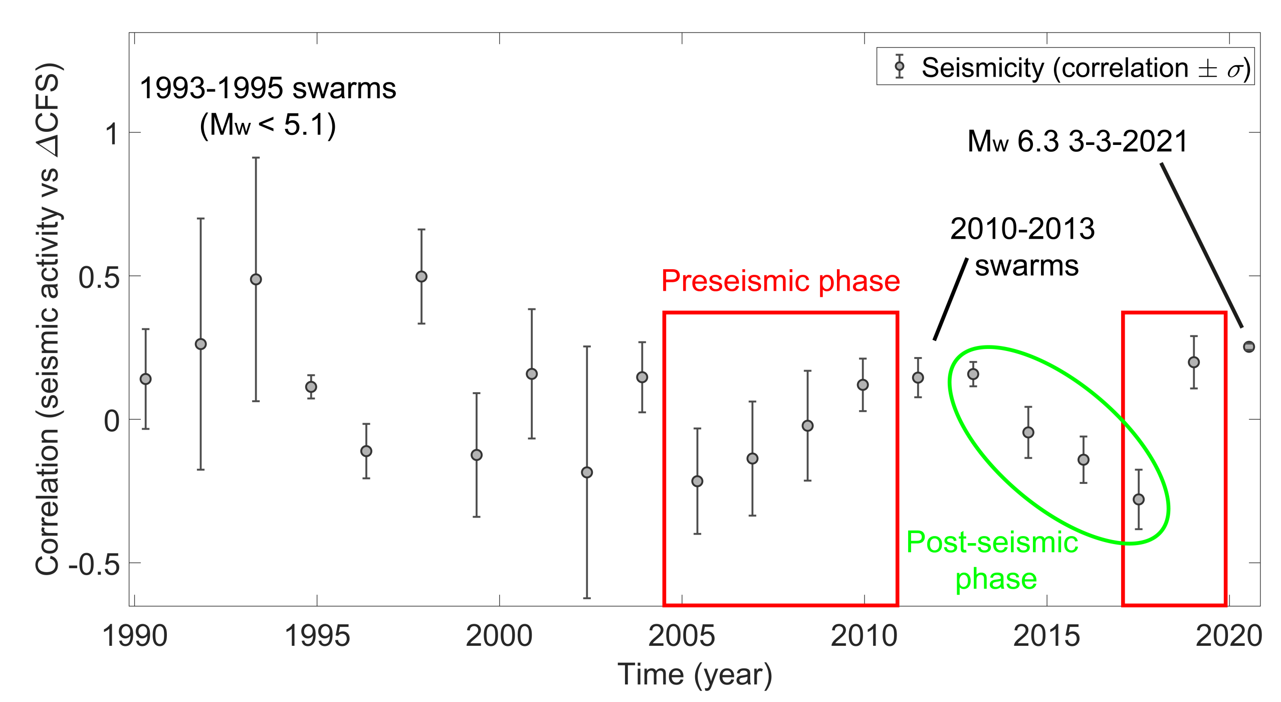
Northern Thessaly Region was recently hit by the Larissa seismic sequence (mainshock 3 March 2021, M 6.3, 11.5 km depth, USGS), causing widespread damage and one casualty. The still ongoing seismicity occurred along normal faulting. The analysis of correlation between the CFS and the nucleated seismic energy is performed between 1990 and 1 May 2021 in an area within latitude 39.5–40.2° N and longitude 21.7–22.4° E considering only earthquakes with M > 2.0. After an initial period featured by elevated correlation values corresponding to a seismic swarm (M≤ 5.0, 0.45) which occurred between 1993 and 1995, a decennial decrease of correlation followed. The trend switched in 2005–2007 and continued till the correlation turns positive. The progressive increase stopped in 2010 when diffuse swarms were recorded.
Then, tidal correlation becomes negative again till 2020, when a peak is rapidly reached at the beginning of 2021 ( 0.29), when Thessaly was shaken by a M 6.3 earthquake. Our results are summarized in Figure 1.
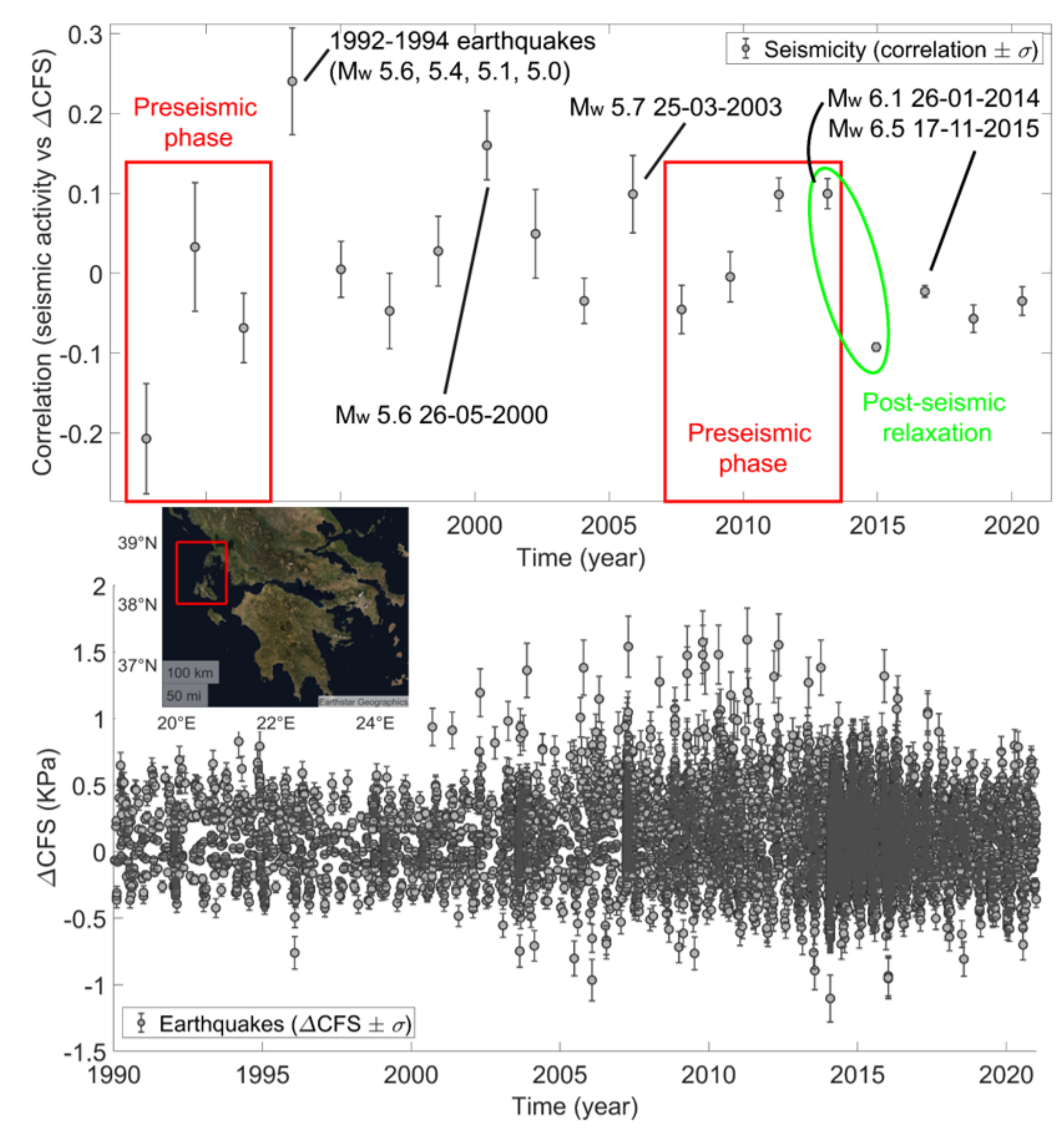
Northern Ionian Greek Islands are often involved by seismic sequences because they rise along the regional plate boundary between the Africa and Eurasia plates, which converge at a rate of about 9 mm/yr towards the north-north west.
Nubian lithosphere subducts beneath the Aegean Sea along the Hellenic Arc.
Focal mechanisms clearly denote compressive earthquakes. The largest seismic events during since 1990 occurred on 17 November 2015, M 6.5 [37], and it is usually known as the Lefkada earthquake because it resulted in several fatalities and dozens injuries on the Greek Island of Lefkada.
This major seismic crisis was forerun by a two-years-long seismic instability, which also included large-magnitude events such as the Cephalonia earthquake (26 January 2014, M 6.1).
Correlation analysis shows an about five years lasting increase of , which reached its maximum in 2013 ( 0.13), then a sharp fall is observed so that tidal correlation becomes compatible with zero. Our results are in Figure 2.
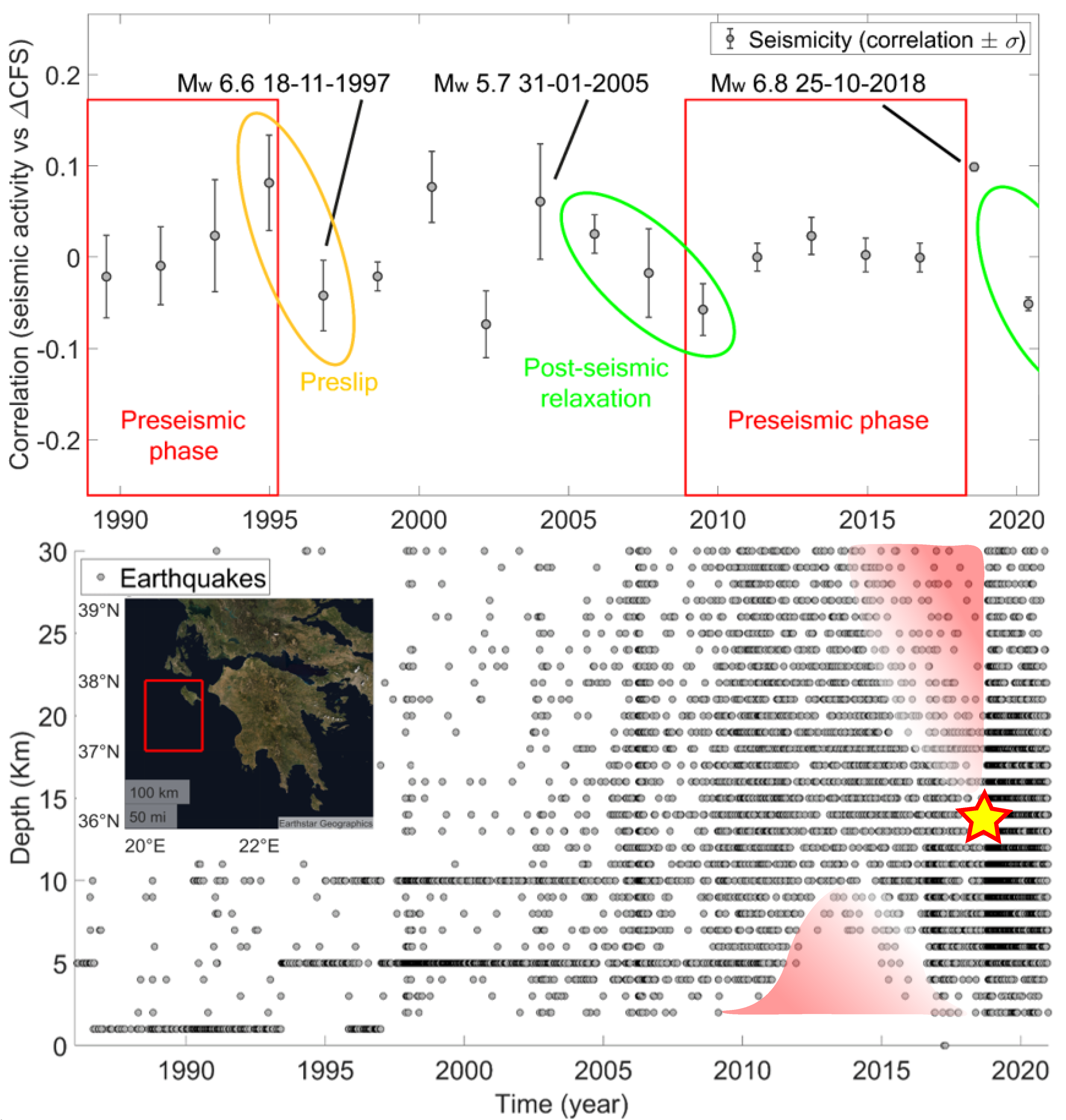
The tectonic setting of the Southern Ioanian Greek Islands (37.0–38.0° N, 20.0–21.0° E) is similar to the previous one.
Great part of seismicity is still featured by a compressive focal mechanism even if a fraction of crustal events with significant oblique component are recordered.
In this territory, two main quakes happened in the last thirty years.
The largest hit Lithakia on 25 October 2018 with M 6.8, depth 15 km, it also produced a small tsunami with about ∼20 cm high anomalous waves.
The other was a M 6.6 earthquake occurred in the same area on 18 November 1997.
The Lithakia earthquake was preceded by an about 7–9 years long period of progressively increase of the tidal correlation between CFS and seismic energy. The peak of the correlation was measured between 2018 and 2019 with 0.11, then a fast decrease is observed.
At the same time, an anomaly in the localization of seismicity is noticed, which is reported in the lower part of Figure 3. Two seismic shadow zones are located at a depth of 0–10 km (2012–2017) and below 19 km (2015–2018).
The seismic quiescence [38] in the forementioned layers is statistically significant especially in the upper one, where the reduction of the seismic rate reached 60% with respect to the preceding 2007–2012 period.
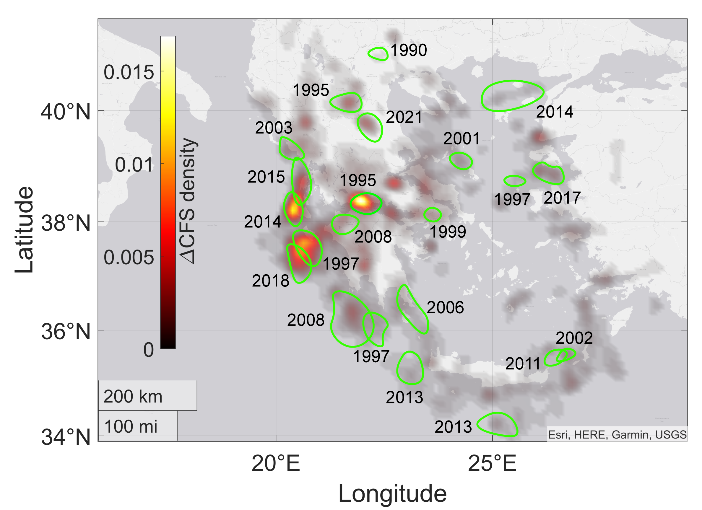
Observations suggest that tends to increase during the preparatory phase of significant crustal earthquakes in Greece. The values of correlation are higher in extensional tectonic settings rather than compressive ones of about 100–200%, normal fault quakes are found to correlate stronger with tidal stress modulations also in other regions. The energy conditions are instead stricter for events occurring in a compressive tectonic setting, so it is reasonable to expect that they correlate very little with the intensity of tidal perturbations, especially in the case of deep hypocenters. Therefore, even though correlations are weak, their modulations can provide precious information about the condition of instability of local crustal volumes, especially if jointly analyzed with other seismological and geodetic recordings. We also analyze the spatial density of the Coulomb stress variation induced by the action of tidal perturbations. For each seismic event, CFS value is calculated, then a map is created that shows the fraction of CFS generated in each location of the selected region. Therefore, the areas with elevated CFS density are those in which seismicity has statistically occurred at more elevated Coulomb stress values or characterized by higher seismicity rate with respect to the surrounding areas.
Since the seismic rate is ultimately controlled by the maximum nucleated magnitude, for each case study, we also plot the areas hit by earthquakes with large magnitude, as written in the caption according to the relative intensity of the regional seismicity. The green contours are drawn according to the finite fault maps of the USGS catalog. Whenever earthquake sequences occur at significantly high CFS values, the brightest spots (according to the vertical colorbar on the left in Figure 4) are located within the green profiles, which suggest self-triggering. On the contrary, shiny stains just outside the main shock areas point out zones featured by elevated stress transfer.
The CFS density map for Greece shows diffuse signal sometimes due to strong motion recordings (e.g., Gulf of Corinth seismic sequence, 1995, and Ionian Arc seismicity in 1997); nevertheless, no correlation is found between the intensity of the signal and large magnitudes, as proven in the cases of the Methoni M 6.9 earthquake and the Aegean Sea M 6.9 event.
4. Discussion
Tidal triggering of earthquakes is still a debated theme in Solid Earth Geophysics. In particular, there are three sources of discussion among geophysicists:
- From a statistical viewpoint, earthquake catalogs are often insufficient to detect significant modulations of seismic activity over time.Tides are tiny perturbations of the gravitational field (0.1–100 kPa) with respect to typical earthquake stress drops (1–50 MPa), but nonetheless they are able to generate significant stress variation rates (∼100 mbar/day compared with 1–10 mbar/day due to tectonic stress, [39]). However, the actual impact on the stability of rock volumes largely depends on the tectonic setting, the spatial orientation of the fault, the depth, and the hypocentral latitude; finally, also the magnitude of the impending event modifies the response of the system to the tidal perturbation. Therefore, a wide range of results were found in several geographical regions.
- It is sometimes difficult to distinguish between the effects of Solid Earth tides from those of ocean tides. Even though the stress amplitude of liquid tides (up to 100 kPa) often exceeds that of the Solid Earth tide (usually ∼0.1–1 kPa), the mechanism of action is quite different. In the first case, tides are concentrated on limited surfaces, at most of the order km, and act mainly through the vertical component, which is transmitted to the horizontal components (almost symmetrically) thanks to the elastic properties of the lithosphere. However, the incremental stress decreases exponentially as depth increases, therefore it can strongly modulate shallow oceanic small magnitude seismicity, for example, at ocean ridges or submarine volcanoes, but it is unlikely that intermediate and deep earthquakes might be triggered by liquid tides.Solid tides, on the other hand, deform the outer layers of the planet mainly in the horizontal components, acting on very large surfaces. For this reason, solid tides have a dominant role in triggering earthquakes except for the just cited peculiar cases. For these reasons, liquid tides are neglected in this work.
- Seismic response to tidal loading strongly depends on the duration of earthquake nucleation.
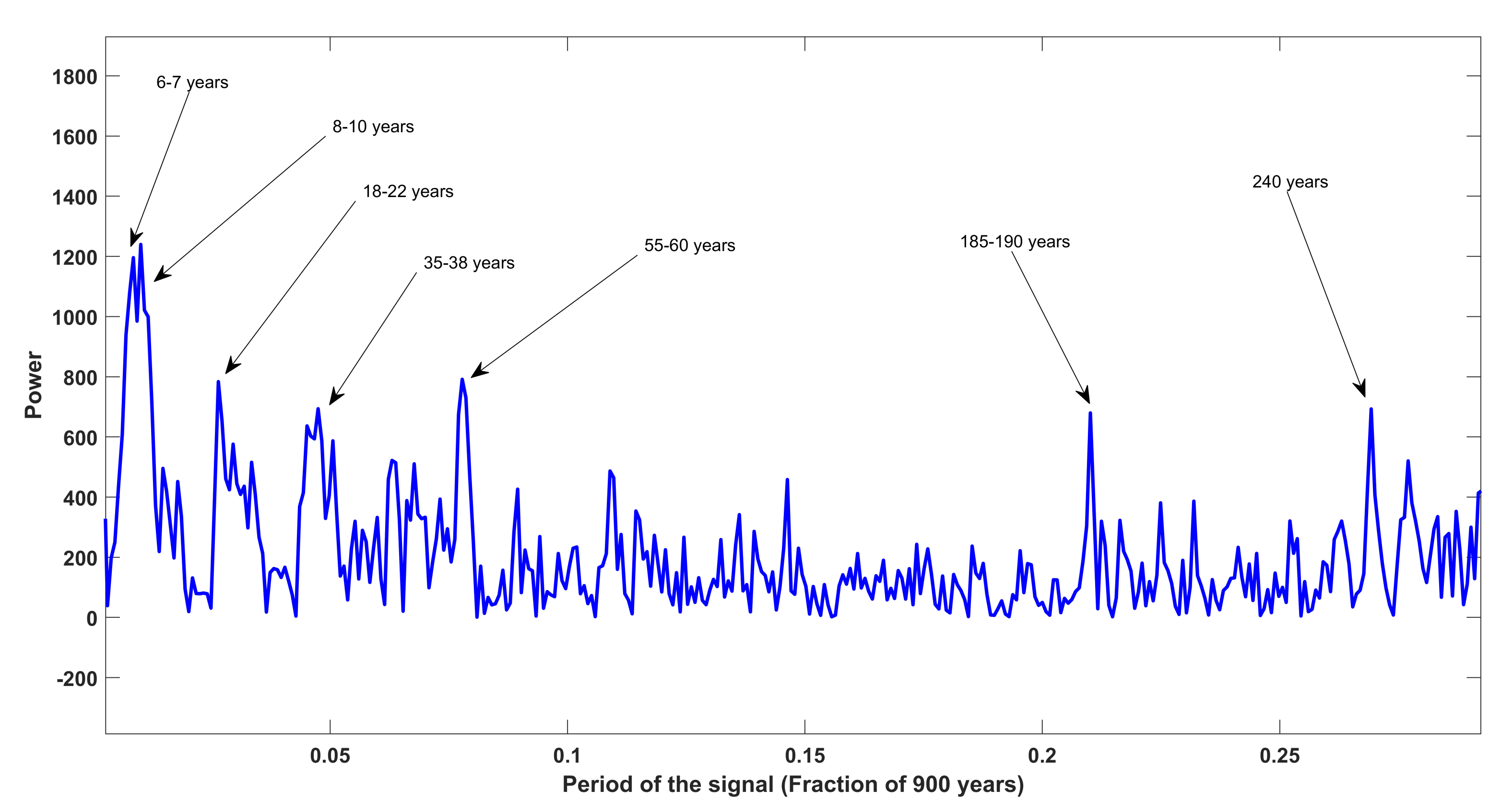
Beyond the aforementioned issues, well-established scientific evidence exists about tidal synchronization in seismic catalogs, as already discussed in the introduction. Both global and regional seismic series show semiannual, annual, biennial, with approximately 9-, 19-, 37-, and 56-years-long periods activity modulations. While the first three frequencies are generally associated with seasonal patterns, the others have no explanation other than lunisolar tidal loading. The FFT of European magnitudes (SHEEC 2020 catalogue) in Figure 6 clearly attests this phenomenon. Since M≈ 6 for the SHEEC catalogue, the nonuniform FFT is applied to include at least M > 5.0. Instrumental recordings are rarely available before the 1950s also for violent earthquakes, and therefore, macroseismic intensity data are widely used combined with epicentral macroseismic intensities and other parametric data sources. Therefore, parametric catalogs must be used with caution and results must be interpreted according to their reliability. Even if an accurate analysis cannot be performed for the aforementioned reasons, the power spectrum of the European seismicity shows typical tidal frequencies such as 8–10- or 18–19-years-long periodicities and some multiples. Moreover, local seismic rates are noticed to be directly correlated with the phase of tidal shear stress or the Coulomb failure stress change in submarine volcanic seismicity [31] and seismic tremors [6]. Finally, it is reasonable to expect that the triggering power of tides is affected by the following variables:
- The critical stress needed for crack propagation depends on the tectonic setting.Then normal-fault quakes and oblique flat or low-angle thrust earthquakes are the most sensible to tidal stress changes [40];
- Lithostatic loading increases with a vertical gradient equal to ∼27 MPa/km, so that confinement stress requires higher and higher energy activation for fracturing (we assume to investigate only crustal volumes above the BDT). If pore pressure is neglected, as a first approximation, earthquakes become less and less susceptible both to ocean and to solid tidal loading with increasing depth;
- Tesseral, sectoral, and zonal components of solid tides reach different amplitudes depending on the latitude, and therefore the intensity of the phenomenon is more or less evident depending on the location.
To perform a reliable statistical analysis
events are required if we assume 1–10 MPa, 0.1–1 kPa and k (compare with [10], p. 12). This means that only high-quality and extended seismological networks can provide an adequate amount of information for our research. Microseismicity strongly correlate with the phase of tidal loading (e.g., [41]), but we neglected this phenomenon in the present work to focus on tectonic earthquakes. Several studies proved a strong sensitivity of seismicity to stress changes of both endogenous and exogenous origins (e.g., [42]). For this reason, Coulomb failure stress was applied to correlate its variations with changes in aftershocks productivity. A difference between static and dynamic Coulomb stress is conventionally done: when loading is slow, so that its increasing/decreasing rate is negligible with respect to the compared time interval, then the static Coulomb stress is at work, on the contrary, if loading occurs suddenly (i.e., fluid injection, coseismic slip), then the dynamic Coulomb failure stress plays a relevant role. In general, the strain produced by earthquakes induces dynamic Coulomb stress swings that, at long distances, can be even an order of magnitude larger than the static stress changes. There is a nonlinear dependence of the time to instability on stress variations [14]; this not only means that seismic rate is a direct effect of loading, but also implies that small additional stress can result in highly unpredictable states of crustal instability. From a mathematical viewpoint, these properties can be summarized in the seismicity rate equation, which, in the simplest form, reads [43]
where is initial seismic rate, is a constitutive parameter, and is the duration of the loading.
In brief, observations suggest that seismicity rate can be influenced by both static and dynamic perturbations. If static stress changes act on crustal stability modulating earthquake occurrence, then seismicity rates might be influenced by the Solid Earth tides, caused by the pull of both the Sun and Moon, even though rather weak with respect to tectonic stress. This is the reason why a research looking for tidal static stress loading signatures along the seismic cycle is meaningful and the results showed in this work can be reliable. The case studies we consider suggest that clustered shallow seismicity tends to occur in correspondence with positive values of the correlation between nucleated seismic energy and CFS. The correlation values show progressive growth before major seismic sequences, while they fall while seismicity is ongoing. Preslip, in agreement with [44], and aftershock activity are also both associated with the lowering of correlation values. On the contrary, seems to increase during quiescent periods, which is compatible with [45]. We think that locked faults become more and more sensitive to stress perturbation as they reach the breaking point, which can provide a simple explanation to the observed trends of .
In summary, we develop a method to highlight the different phases of the seismic cycle in fault systems by studying their response to a well-known stress perturbation, i.e., tidal stress. Even though seismic prediction was considered impossible [46], no theoretical reason prevents it. Since the physics of fracture at seismological spatio-temporal scale is still poorly understood and no unique mechanism for nucleation was proven to exist, then seismic precursors cannot be effective in predicting impending earthquakes. By the same token, it is unlikely that the probability of occurrence of single earthquakes may ever be reliably assessed. However, it was proven, also in this article, that fault systems change their mechanical response during the different phases of seismic activity, which is certainly not sufficient for forecasting, but it can be used to understand whether fault systems are evolving towards instability. Our analysis shows that a preseismic phase is observed before large and intermediate (M 5) shallow (depth km) earthquakes. Therefore, our advances achieved in this research are significant, with a potential impact on seismic hazards. In addition, they provide new insights for the comprehension of the relationship between stress perturbations, earthquake nucleation, and seismic sequences, which are still to be fully investigated.
Author Contributions
Conceptualization, D.Z. and C.D.; methodology, D.Z. and L.T.; data analysis, D.Z.; writing—original draft preparation, D.Z.; writing—review and editing, C.D. and L.T.; supervision, C.D. and L.T. All authors have read and agreed to the published version of the manuscript.
Funding
This research was funded by ESA through the TILDE Project.
Data Availability Statement
We used free data available at several seismological catalogs, as written inside the text.
Acknowledgments
Discussions with G. Nico, F.G. Panza, F. Ricci, and F. Vespe were precious.
Conflicts of Interest
The authors declare no conflict of interest. This work was developed as part of the TILDE project, ESA. The funders had no role in the design of the study; in the collection, analyses, or interpretation of data; in the writing of the manuscript, or in the decision to publish the results.
References
- De Geus, T.W.; Popović, M.; Ji, W.; Rosso, A.; Wyart, M. How collective asperity detachments nucleate slip at frictional interfaces. Proc. Natl. Acad. Sci. USA 2019, 116, 23977–23983. [Google Scholar] [CrossRef] [Green Version]
- Ellsworth, W.L. Injection-induced earthquakes. Science 2013, 341, 1225942. [Google Scholar] [CrossRef]
- Varga, P.; Grafarend, E. Influence of tidal forces on the triggering of seismic events. In Geodynamics and Earth Tides Observations from Global to Micro Scale; Birkhäuser: Cham, Switzerland, 2019; pp. 55–63. [Google Scholar]
- Tanaka, S.; Ohtake, M.; Sato, H. Evidence for tidal triggering of earthquakes as revealed from statistical analysis of global data. J. Geophys. Res. 2002, 107, 2211. [Google Scholar] [CrossRef] [Green Version]
- Heaton, T.H. Tidal triggering of earthquakes. Geophys. J. Int. 1975, 43, 307–326. [Google Scholar] [CrossRef] [Green Version]
- Rubinstein, J.L.; La Rocca, M.; Vidale, J.E.; Creager, K.C.; Wech, A.G. Tidal modulation of nonvolcanic tremor. Science 2008, 319, 186–189. [Google Scholar] [CrossRef] [Green Version]
- Métivier, L.; de Viron, O.; Conrad, C.P.; Renault, S.; Diament, M.; Patau, G. Evidence of earthquake triggering by the solid earth tides. Earth Planet. Sci. Lett. 2009, 278, 370–375. [Google Scholar] [CrossRef]
- Ide, S.; Yabe, S.; Tanaka, Y. Earthquake potential revealed by tidal influence on earthquake size–frequency statistics. Nat. Geosci. 2016, 9, 834–837. [Google Scholar] [CrossRef]
- Kossobokov, V.G.; Panza, G.F. A myth of preferred days of strong earthquakes? Seism. Res. Lett. 2020, 91, 948–955. [Google Scholar] [CrossRef]
- Beeler, N.M.; Lockner, D.A. Why earthquakes correlate weakly with the solid Earth tides: Effects of periodic stress on the rate and probability of earthquake occurrence. J. Geophys. Res. 2003, 108, 2391. [Google Scholar] [CrossRef] [Green Version]
- Munk, W. Once again: Once again tidal friction. Prog. Oceanogr. 1997, 40, 7–35. [Google Scholar] [CrossRef]
- Smith, S.W.; Jungels, P. Phase delay of the solid earth tide. Phys. Earth Planet. Inter. 1970, 2, 233–238. [Google Scholar] [CrossRef]
- Doglioni, C. The global tectonic pattern. J. Geodyn. 1990, 12, 21–38. [Google Scholar] [CrossRef]
- Dieterich, J.H. Nucleation and triggering of earthquake slip: Effect of periodic stresses. Tectonophysics 1987, 144, 127–139. [Google Scholar] [CrossRef]
- Cochran, E.S.; Vidale, J.E.; Tanaka, S. Earth tides can trigger shallow thrust fault earthquakes. Science 2004, 306, 1164–1166. [Google Scholar] [CrossRef] [Green Version]
- Bendick, R.; Mencin, D. Evidence for synchronization in the global earthquake catalog. Geophys. Res. Lett. 2020, 47, e2020GL087129. [Google Scholar] [CrossRef]
- Ide, S.; Tanaka, Y. Controls on plate motion by oscillating tidal stress: Evidence from deep tremors in western Japan. Geophys. Res. Lett. 2014, 41, 3842–3850. [Google Scholar] [CrossRef]
- Zaccagnino, D.; Vespe, F.; Doglioni, C. Tidal modulation of plate motions. Earth Sci. Rev. 2020, 205, 103179. [Google Scholar] [CrossRef]
- Wiemer, S.; Wyss, M. Minimum magnitude of completeness in earthquake catalogs: Examples from Alaska, the western United States, and Japan. Bull. Seismol. Soc. Am. 2000, 90, 859–869. [Google Scholar] [CrossRef]
- Trotta, J.; Tullis, T. An Independent Assessment of the Load/Unload Response Ratio (LURR) Proposed Method of Earthquake Prediction. Pure Appl. Geophys. 2006, 163, 2375–2387. [Google Scholar] [CrossRef]
- Tanaka, S. Tidal triggering of earthquakes prior to the 2011 Tohoku-Oki earthquake (Mw 9.1). Geophys. Res. Lett. 2012, 39. [Google Scholar] [CrossRef]
- Su, B.; Li, H.; Ma, W.; Zhao, J.; Yao, Q.; Cui, J.; Yue, C.; Kang, C. The Outgoing Longwave Radiation Analysis of Medium and Strong Earthquakes. IEEE J. Sel. Top. Appl. Earth Obs. Remote Sens. 2021, 14, 6962–6973. [Google Scholar] [CrossRef]
- Baker, T.F. Tidal deformations of the Earth. Sci. Prog. 1984, 69, 197–233. [Google Scholar]
- Doodson, A.T. The harmonic development of the tide-generating potential. Proc. R. Soc. Lond. 1921, 100, 305–329. [Google Scholar]
- Agnew, D.C. Earth Tides. In Treatise on Geophysics, Volume 3: Geodesy; Elsevier: Amsterdam, The Netherlands, 2010; pp. 163–195. [Google Scholar]
- Tsuruoka, H.; Ohtake, M.; Sato, H. Statistical test of the tidal triggering of earthquakes: Contribution of the ocean tide loading effect. Geophys. J. Int. 1995, 122, 183–194. [Google Scholar] [CrossRef]
- Takeuchi, H.; Saito, M. Seismic surface waves. Method Comp. Phys. 1972, 11, 217–295. [Google Scholar]
- Dziewonski, A.M.; Anderson, D.L. Preliminary reference Earth model. Phys. Earth Planet. Inter. 1981, 25, 297–356. [Google Scholar] [CrossRef]
- Lambert, A.; Kao, H.; Rogers, G.; Courtier, N. Correlation of tremor activity with tidal stress in the northern Cascadia subduction zone. J. Geophys. Res. 2009, 114. [Google Scholar] [CrossRef] [Green Version]
- Tan, Y.J.; Waldhauser, F.; Tolstoy, M.; Wilcock, W.S. Axial Seamount: Periodic tidal loading reveals stress dependence of the earthquake size distribution (b value). Earth Planet. Sci. Lett. 2019, 512, 39–45. [Google Scholar] [CrossRef] [Green Version]
- Scholz, C.H.; Tan, Y.J.; Albino, F. The mechanism of tidal triggering of earthquakes at mid-ocean ridges. Nat. Commun. 2019, 10, 1–7. [Google Scholar] [CrossRef] [Green Version]
- Matsumoto, K.; Takanezawa, T.; Ooe, M. Ocean tide models developed by assimilating TOPEX/POSEIDON altimeter data into hydrodynamical model: A global model and a regional model around Japan. J. Oceanogr. 2000, 56, 567–581. [Google Scholar] [CrossRef]
- Oppenheimer, D.H.; Reasenberg, P.A.; Simpson, R.W. Fault plane solutions for the 1984 Morgan Hill, California, earthquake sequence: Evidence for the state of stress on the Calaveras fault. J. Geophys. Res. 1988, 93, 9007–9026. [Google Scholar] [CrossRef]
- Harris, R.A. Earthquake stress triggers, stress shadows, and seismic hazard. Curr. Sci. 2000, 79, 1215–1225. [Google Scholar]
- King, G.C.; Stein, R.S.; Lin, J. Static stress changes and the triggering of earthquakes. Bull. Seismol. Soc. Am. 1994, 84, 935–953. [Google Scholar]
- Arabelos, D.N.; Papazachariou, D.Z.; Contadakis, M.E.; Spatalas, S.D. A new tide model for the Mediterranean Sea based on altimetry and tide gauge assimilation. Ocean Sci. 2011, 7, 429–444. [Google Scholar] [CrossRef] [Green Version]
- Chousianitis, K.; Konca, A.O.; Tselentis, G.A.; Papadopoulos, G.A.; Gianniou, M. Slip model of the 17 November 2015 Mw= 6.5 Lefkada earthquake from the joint inversion of geodetic and seismic data. Geophys. Res. Lett. 2016, 43, 7973–7981. [Google Scholar] [CrossRef] [Green Version]
- Reasenberg, P.A.; Matthews, M.V. Precursory seismic quiescence: A preliminary assessment of the hypothesis. Pure Appl. Geophys. 1988, 126, 373–406. [Google Scholar] [CrossRef]
- Varga, P.; Grafarend, E. Distribution of the lunisolar tidal elastic stress tensor components within the Earth’s mantle. Phys. Earth Planet. Inter. 1996, 93, 285–297. [Google Scholar] [CrossRef]
- Doglioni, C.; Carminati, E.; Petricca, P.; Riguzzi, F. Normal fault earthquakes or graviquakes. Sci. Rep. 2015, 5, 1–12. [Google Scholar] [CrossRef]
- Pétrélis, F.; Chanard, K.; Schubnel, A.; Hatano, T. Earthquake sensitivity to tides and seasons: Theoretical studies. J. Stat. Mech. Theory Exp. 2021, 2021, 023404. [Google Scholar] [CrossRef]
- Thomas, A.M.; Bürgmann, R.; Shelly, D.R.; Beeler, N.M.; Rudolph, M.L. Tidal triggering of low frequency earthquakes near Parkfield, California: Implications for fault mechanics within the brittle-ductile transition. J. Geophys. Res. 2012, 117, 1–24. [Google Scholar] [CrossRef]
- Stein, R.S. The role of stress transfer in earthquake occurrence. Nature 1999, 402, 605–609. [Google Scholar] [CrossRef]
- Ellsworth, W.L.; Beroza, G.C. Seismic evidence for an earthquake nucleation phase. Science 1995, 268, 851–855. [Google Scholar] [CrossRef] [PubMed]
- Mignan, A.; Di Giovambattista, R. Relationship between accelerating seismicity and quiescence, two precursors to large earthquakes. Geophys. Res. Lett. 2008, 35. [Google Scholar] [CrossRef]
- Geller, R.J.; Jackson, D.D.; Kagan, Y.Y.; Mulargia, F. Earthquakes cannot be predicted. Science 1997, 275, 1616. [Google Scholar] [CrossRef] [Green Version]
Figure 1.
Correlation between CFS and seismicity in Thessaly Greece, between 1990 and 2021, M, NOAIG Catalog.
Figure 1.
Correlation between CFS and seismicity in Thessaly Greece, between 1990 and 2021, M, NOAIG Catalog.

Figure 2.
(Top) correlation between CFS and seismicity close to the Greek Ionian coasts (38.0–39.0° N, 20.0–21.0° E, M > 2.0, NOAIG Catalog.) between 1990 and 2021. Main event was located in southwestern region of Lefkada Island between the villages Athani and Agios Petros. The 2014–2016 seismic sequence involved faults within different tectonic settings. (Bottom) CFS as a function of time. Before the 2014–2016 seismic sequence, significant changes in the Coulomb stress distribution was observed, partially due to contribution of deeper (>20 km) earthquakes.

Figure 3.
Correlation between CFS and seismicity close to the Greek Ionian coasts (37.0–38.0° N, 20.0–21.0° E) between 1985 and 2021. A nine-years-long preseismic phase is highlighted both by an increasing value of correlation in the upper part of the picture, and seismic quiescence, represented by two red shadow zones, at a depth of 0–10 km (2012–2017) and >20 km (2015–2018). The yellow star represents the M 6.8, 25 October 2018 Lithakia mainshock.

Figure 4.
CFS density map for seismicity in Greece, NOAIG Catalog, 1990–2021, M 2.0. Highest density areas are located on the Greek Ionian Islands along Hellenic Trench and along normal fault system of Gulf of Corinth.
Figure 4.
CFS density map for seismicity in Greece, NOAIG Catalog, 1990–2021, M 2.0. Highest density areas are located on the Greek Ionian Islands along Hellenic Trench and along normal fault system of Gulf of Corinth.

Figure 5.
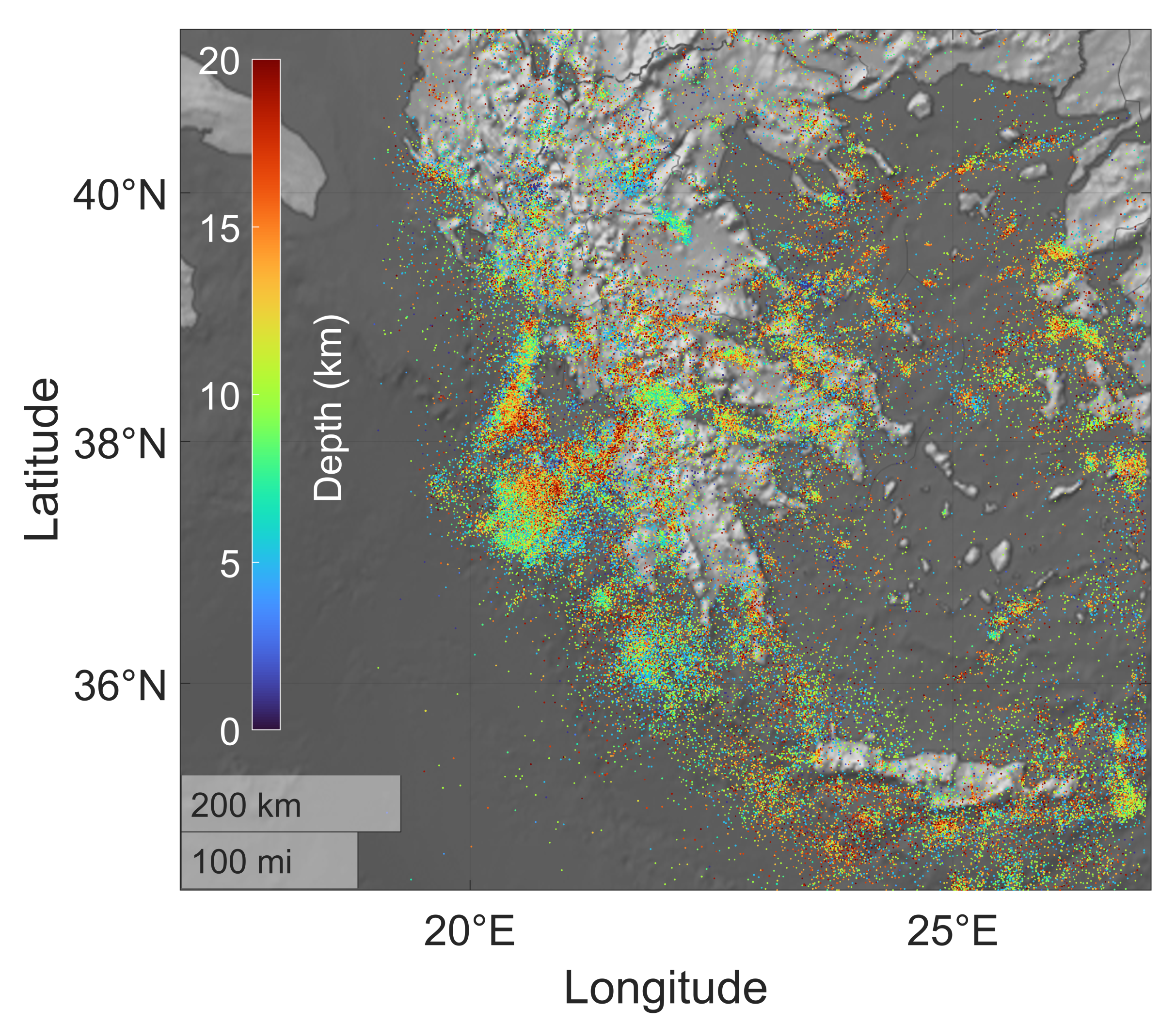
Map of seismicity in Greece between 1990 and 1/8/2021, M > 2.0, NOAIG Catalogue.

Figure 6.
Power spectrum of European seismicity (M > 5.0, 1106–2006, SHEEC catalogue). Tidal periodicities are detected in the recurrence times of intense seismicity in Europe. nuFFT is used for the calculation to take into account progressive decrease of completeness magnitude.
Figure 6.
Power spectrum of European seismicity (M > 5.0, 1106–2006, SHEEC catalogue). Tidal periodicities are detected in the recurrence times of intense seismicity in Europe. nuFFT is used for the calculation to take into account progressive decrease of completeness magnitude.


Table 1.
Largest tidal frequencies.
| Symbol | Doodson Number | Period (Days) | Amplitude (m) |
|---|---|---|---|
| 2 5 5 5 5 5 | 0.518 | 0.6322 | |
| 2 7 3 5 5 5 | 0.500 | 0.2941 | |
| 1 6 5 5 5 5 | 0.997 | 0.3686 | |
| M | 0 7 5 5 5 5 | 13.661 | − 0.0666 |
| M | 0 6 5 4 5 5 | 27.555 | − 0.0352 |
| SSa | 0 5 7 5 5 5 | 182.622 | − 0.0310 |
| h | 0 5 6 5 5 4 | 365.264 | − 0.0049 |
| p | 0 5 5 6 5 5 | 3232.605 | 0.0002 |
| N/2 | 0 5 5 5 7 5 | 3399.048 | − 0.0003 |
| N | 0 5 5 5 6 5 | 6798.097 | 0.0279 |
Publisher’s Note: MDPI stays neutral with regard to jurisdictional claims in published maps and institutional affiliations. |
© 2021 by the authors. Licensee MDPI, Basel, Switzerland. This article is an open access article distributed under the terms and conditions of the Creative Commons Attribution (CC BY) license (https://creativecommons.org/licenses/by/4.0/).
Share and Cite
MDPI and ACS Style
Zaccagnino, D.; Telesca, L.; Doglioni, C. Different Fault Response to Stress during the Seismic Cycle. Appl. Sci. 2021, 11, 9596. https://doi.org/10.3390/app11209596
AMA Style
Zaccagnino D, Telesca L, Doglioni C. Different Fault Response to Stress during the Seismic Cycle. Applied Sciences. 2021; 11(20):9596. https://doi.org/10.3390/app11209596
Chicago/Turabian StyleZaccagnino, Davide, Luciano Telesca, and Carlo Doglioni. 2021. "Different Fault Response to Stress during the Seismic Cycle" Applied Sciences 11, no. 20: 9596. https://doi.org/10.3390/app11209596
Note that from the first issue of 2016, this journal uses article numbers instead of page numbers. See further details here.