Article

Acoustic Emission Signal Due to Fiber Break and Fiber Matrix Debonding in Model Composite: A Computational Study

1
INSA de Lyon, University of Lyon, MATEIS UMR 5510, F-69621 Villeurbanne, France
2
INSA-Lyon, University of Lyon, LVA EA677, F-69621 Villeurbanne, France
*
Author to whom correspondence should be addressed.
Appl. Sci. 2021, 11(18), 8406; https://doi.org/10.3390/app11188406
Submission received: 16 July 2021 / Revised: 6 September 2021 / Accepted: 8 September 2021 / Published: 10 September 2021

Abstract

:
Acoustic emission monitoring is a useful technique to deal with detection and identification of damage in composite materials. Over the last few years, identification of damage through intelligent signal processing was particularly emphasized. Data-driven models are developed to predict the remaining useful lifetime. Finite elements modeling (FEM) was used to simulate AE signals due to fiber break and fiber/matrix debonding in a model carbon fiber composite and thereby better understand the AE signals and physical phenomena. This paper presents a computational analysis of AE waveforms resulting from fiber break and fiber/matrix debonding. The objective of this research was to compare the AE signals from a validated fiber break simulation to the AE signals obtained from fiber/matrix debonding and fiber break obtained in several media and to discuss the capability to detect and identify each source.

1. Introduction

Composite materials are used in several applications such as aircraft structural components or in civil infrastructures due to their high structural performance. These materials may exhibit damage mechanisms such as matrix cracking, fiber break, fiber/matrix debonding and delamination. Real-time monitoring of composite damage is thus of primary importance to prevent failure. Prognostics and health management (PHM) of components involve both diagnostic and prognostic steps [1,2]. Diagnostics consist in detecting and identifying the different damage mechanisms. This step is crucial for the reliability of these structures [3,4] and ensuring successful prognostic strategies, which still need to be developed [5,6,7]. These methods exploit the data measured by a network of sensors located on the structure in order to determine the damage state; then, the prognostic strategies can predict the remaining useful lifetime (RUL) of the structure [8,9]. This procedure involves several steps: damage (1) detection, (2) localization, (3) classification and quantification and, finally, (4) prognostics. Therefore, damage detection and identification are crucial steps to perform prognostics and RUL prediction. An acceptable prognostic method starts with robust diagnostics, since any future predictions are affected by the uncertainties in the estimated damage state or wrong identification of damage mechanisms.
Real-time monitoring of composite damage may be carried out using Acoustic Emission (AE), whose principle is described hereafter. Damage occurring in composite materials results in the nucleation and propagation of cracks or debonding and thus energy release. A part of this energy is released as elastic waves that propagate through the material.
These waves can be detected by sensors that are placed on the surface of the specimen. Damage mechanisms thus act as acoustic emission sources. A main advantage of AE is the possibility to detect damage in situ even at an early stage in a nondestructive manner. However, the main difficulty consists in establishing a robust link between the different damage mechanisms and the signals acquired by the sensors. In common practice, most of the AE analysis is based on an empirical approach which consists of gathering AE signals with similar characteristics into groups and assuming that each group corresponds to a given damage mechanism. These correlations between the sources and the AE signals generally lack validity. Indeed, few AE signal labels are confirmed by direct observations of the sources due to the difficulty of experimentally controlling the sources. Nevertheless, the possibility of identifying AE signatures of damage mechanisms is an established field [10,11,12,13,14,15,16].
The diagnostic phase consists of data acquisition, signal processing and features extraction and selection. The main diagnostic challenges in AE monitoring are related to the coexistence of AE signatures due to several damage mechanisms, as well as the numerous features that affect the original signal emitted by the AE source. The finally acquired AE signal is the convolution of the source signal, medium transfer function and sensor transfer function. In fact, AE signals depend on several distinct factors [17,18,19,20,21,22,23]: (1) the damage source, (2) the specimen geometry, (3) the material properties and (4) the type of sensor and instrumentation. The contribution of each of these elements must be considered to correctly analyze the recorded waveforms. Consequently, it is not straightforward to establish a quantitative link between the damage sources and AE signals, and further investigations are needed to enrich the existing experimental studies on this topic. Modeling and numerical simulations of AE appear as a promising way to reach this objective [24,25,26,27,28,29,30,31,32,33,34,35,36,37,38,39,40,41].
The first works about modeling an AE source were based on analytic and semi-analytic methods. Ono and Ohtsu [30] developed a generalized theory of AE based on the integral formulation of elastodynamics. The AE sources were considered as a single point buried in the structure. To model the different crack modes, a moment tensor was defined on this point based on a multiscale approach and various source-time functions to model the source kinematics. Suzuki et al. [39] extended the analyses to a dissipative medium including a relaxation function. Giordano et al. [42] developed a model for AE wave propagation based on the ray theory, applied in plates with viscoelastic properties. Numerical methods were then used to simulate the sources of AE. Dietzhausen et al. [25] investigated the dynamic behaviour due to a single glass fiber break in a polymer matrix using the finite element (FE) method and carried out parametric studies with different matrix material laws (elastic, nonlinear elastic and elastic-plastic model) and various fiber positions in the thickness of the specimen. A dynamic FE approach was developed for the prediction of AE waveforms in the far field plates [26,28]. Sause et al. [33] simulated the AE sources in a composite material using FE methods applying a multiscale approach [27,33,43]. They improved the representation of the sources compared to that of previous works by using a failure criterion to determine the loading resulting in crack propagation [27] and later on by considering the crack geometry determined from μ-Computed Tomography [43].
They also considered the different elements of the acquisition chain, thus enabling a comparison between the signals obtained numerically and experimentally. Such a quantitative comparison cannot be achieved without accounting for the transfer function of the sensor, which can be obtained either from the analytical reciprocity method [44,45] or from multi-physics simulations reproducing the interface between the sensor and the material [46,47,48,49,50].
Numerical simulations of fiber breaks accounting for all the above-mentioned features were recently set up [51]. A specimen made of a single carbon fiber and epoxy matrix [51,52] was used to experimentally validate the fiber break AE signals. The influence of the type of sensor, specimen geometry and AE source location were studied, resulting in a quantitative agreement in both time and frequency domains between numerical and experimental AE signals from fiber break [51].
The objective of this study was to extend the proposed model to account for both fiber break and fiber/matrix debonding as well as to identify the main parameters that influence the acoustic emission signatures.
The organization of the paper is now outlined. After a brief presentation of the experimental tests in Section 2, we present the numerical simulations of fiber break and fiber/matrix debonding as well as the subsequent AE signal propagation and detection in Section 3. In Section 4, AE results are presented and discussed. First, we recall the FE model validation of fiber break. Then, it is extended to study the influence of the matrix properties, the sensor and the damage mechanism on the AE signal and the corresponding descriptors, including the capability of detection and identification of each source.

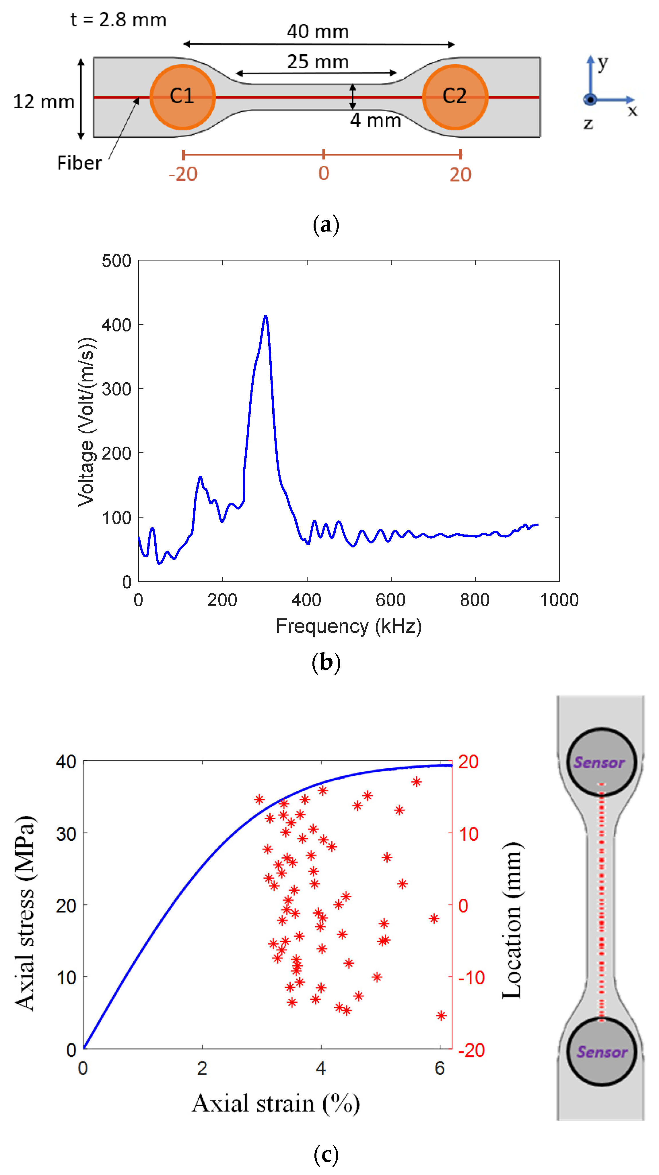
2. Experimental Procedure

The experimental specimens, reported in Figure 1a, consisted of a single long carbon fiber T700 (7 μm in diameter) embedded in an epoxy/amine matrix denoted DGEBD-3DCM. The axes were designated such that the (Ox) axis was along the fiber, the (Oy) axis was normal to the fiber in the plane of the specimen and the (Oz) axis was perpendicular to the plane of the plate. The specimen’s thickness was 2.8 mm. The fiber was centered along the specimen’s width (i.e., it lies in (Oxz) plane) but not along the thickness (i.e., it is shifted along direction (Oz) with respect to (Oxy) plane) since it was located 0.5 mm from the surface along the (Oz) axis. The mechanical tests were carried out at room temperature at a 0.5 mm/min strain rate. AE monitoring was performed using resonant sensors connected to a PCI-2 data acquisition system (Mistras Group, Sucy en Brie, France). Tensile tests were conducted with nano 30 sensors, 40 mm apart (Figure 1a). The sensitivity curve of the sensors is shown in Figure 1b. These sensors show good sensitivity in the frequency range from 200 to 400 kHz (MISTRAS Group data). In all tests, the coupling agent applied on the contact surface of the sensor with the structure was medium-viscosity vacuum grease. All the waveforms were recorded and filtered in the bandwidth 20–1200 kHz (the sampling rate was equal to 5 Msps). Waveform preprocessing consisted of the following steps: pre-trigger removal, tail cutting and Shape Preserving Interpolation (SPI) resampling. Tail cutting consisted of applying a floating threshold equal to 10% of the peak amplitude to determine the end of the signal. The acquisition threshold was 32 dB, and only the signals located along the gauge length were analyzed. Wave velocity was equal to 1750 m/s. More details about the experiments are given in [51]. A one-to-one correlation between the numbers of AE located signals and the observed fiber breaks was established (Figure 1c). Microscope observations resulted in 58 fiber breaks; the largest part was detected by the AE sensors, since 56 signals were located in the gauge length. Every located source originated from a fiber break, and optical observations confirmed the absence of fiber/matrix debonding.

3. Numerical Simulation of AE Signals

Modeling of propagation and attenuation of elastic waves in an elastic medium to predict AE signatures were performed under some assumptions regarding (1) the definition of crack initiation and (2) propagation and attenuation of elastic waves described in the sequel.

3.1. Fiber Break and Surrounding Medium

We first recalled the numerical procedure for fiber break simulation (more details can be found in [51]). A 3D FE model of the single fiber specimen was set up using AbaqusTM Standard, with the same dimensions as those of the experimental specimens. The fiber and matrix behavior were considered linear, elastic and isotropic. The acoustic emission source was a crack in the fiber, covering the whole fiber section and perpendicular to the fiber neutral line. It was located at a distance of 12 mm from the sensor C along the (Ox) direction and 0.5 mm from the top surface along the (Oz) (Figure 2a). The nodes lying on the fiber break plane were doubled so as to enable the surface separation at this location (Figure 2b). A two-step simulation was adopted to represent the fiber break. A quasi-static step was firstly applied. During this step, the imposed force reached the experimentally measured value at first fiber break (i.e., 346 N). Displacement constraints were set on the fiber break plane nodes so that no surface separation was allowed during this step. Then, the displacement constraints on these nodes were released in the second dynamic step (Figure 2b), enabling the surface separation and vibration which resulted in the generation of elastic waves that further propagated within the specimen with possible reflections at the specimen boundaries. Frequencies up to 1 MHz are generally involved in AE analysis, which requires a 0.1 µs maximum time increment in the FE model to be able to accurately represent these waves. Moreover, the FE mesh must contain small enough elements in order to resolve spatial features (from 0.2 mm down to 0.01 mm close to the model source). The simulated waveforms were calculated on single nodes from the epicenter of the source to the boundaries of the gauge length on the top surface (Figure 2a, red line) and at the position of sensor C.
Acoustic waves are subjected to geometric damping where the source energy spreads through a larger volume. Geometric damping is a function of distance and wave type. However, for these specimens, the main source of damping of the AE waves is the dissipation due to the viscoelasticity property of the propagation medium, which can be modeled using Rayleigh parameters. It is a frequency-dependent model, formulated as a combination of mass proportional and stiffness proportional damping (Figure 3). The loss factor ( η R ) is the sum of two terms, one proportional to frequency (multiplicating coefficient αR) and one inversely proportional to frequency (multiplicating coefficient βR). The influence of αR and βR is respectively negligible for high and low frequencies. Figure 3 represents the variation of the damping ratio as a function of the frequency for a given case. The curve shows nonlinearity in the low-frequency regime (<400 kHz), and beyond that, the variation becomes linear due to the domination of the term βRω.
In Section 4, the influence of the surrounding medium on the AE signature due to fiber break is analyzed. In the case of elastic modeling, wave velocity is directly proportional to Young’s modulus of the matrix. The properties of the matrix material were chosen in order to simulate different materials [50,51,52,53,54] such as polymers (denoted as matrix type α), ceramics (denoted as matrix type β), or composite (carbon fiber reinforced polymer, CFRP, denoted as matrix type γ). Table 1 gathers the corresponding material properties used for numerical simulations. The comparison between the different matrices cannot be established based on the same imposed force because of the stiffness differences. Therefore, the imposed force was adapted to ensure the same fiber strain at failure of 2.5%.

3.2. Simulation of Debonding

The FE model was extended to account for fiber/matrix debonding. It can be noted that debonding at the fiber/matrix interface was not observed experimentally in the tested specimens. However, this damage mechanism is usually observed in composite materials and could have been observed with the same constituents but with another fiber surface treatment, for instance. Indeed, the debonding characteristics depend on the quality of the fiber/matrix interface. Since the proposed FE model was quantitatively validated against experimental results in the case of fiber break, we extended it to simulate debonding and assess the influence of the damage mechanism on the AE signal. Several cases of debonding between the epoxy matrix and the fiber were studied. Contrary to fiber break, for which the crack surface was perpendicular to the loading direction, debonding along the fiber surface occurred in a direction that was parallel to the imposed loading direction. Debonding was assumed to occur over the whole fiber/matrix interface along a given length in the fiber direction, centered with respect to the fiber break location. It should be pointed out that debonding was assumed to occur at the same applied load as the one applied for the fiber break, which is usually experimentally observed and confirmed by numerical simulations in composites. These simulations [55] showed that debonding could not occur before cracking because there is not enough stress at the interface and that debonding starts immediately after cracking, thus at the same loading level.
Figure 4 shows different kinetics of debonding. For Model A, several crack lengths were investigated between 20 and 200 μm. First, it was assumed that crack growth was quasi-instantaneous (Figure 4a). In this case, we had a single jump of the debonding. Numerically, the quasi-instantaneous debonding corresponded to a separation of nodes for a duration equal to one calculation time step (0.1 µs). The corresponding debonding velocity thus varied between 200 and 2000 m/s.
The second kind of debonding models dealt with more resistant interfaces (Figure 4b–d). In these cases, debonding occurred gradually (models B–D), with a final debonding length equal to 100 μm. The crack grew by jumps with several steps. The 20 μm extension of the crack was also generated with a node separation during one 0.1 µs time step. For linear progressive debonding in five steps (model B, Figure 4b), the propagation of the debonding at the interface was equal to 20 μm every 0.1 μs. For uniform progressive debonding (model C, Figure 4c), the first propagation was equal to 20 μm in 0.1 μs. The next propagations were assumed to occur after constant periods of 0.2 μs. For non-uniform progressive debonding (model D, Figure 4d), debonding took place also in five steps, 20 μm was generated at each step in 0.1 μs, and the time interval between two crack extensions increased progressively from 0.2 to 2 μs.

3.3. Sensor Simulation

Two types of sensors were considered in the modeling part: a perfect virtual point-contact sensor and resonant sensors.

3.3.1. Perfect Virtual Point-Contact Sensor

Simulated sensors were placed on the top surface, centered with respect to the width of the specimen at various locations from the epicenter of the source to the end of the sample. The first type of sensor corresponded to a pseudo-sensor, a wideband point contact sensor with no resonances, called perfect virtual point-contact sensor. A signal detected by this sensor corresponded to the out-of-plane velocity (vz) calculated on a single node. It was considered as “perfect” because it retained the entire signal that propagated over the surface of the material. The waveforms (out-of-plane velocity vz) were calculated on several nodes from the epicenter of the source to the boundaries of the gauge length on the top surface (Figure 2a). The out-of-plane displacements or velocities at the upper surface were spatially (∆x = 0.2 mm) and temporally (∆t = 0.2 μs) sampled. All numerical signals were filtered with a four-order Butterworth bandpass filter with the bandwidth between 20 and 1200 kHz. For the signal time windowing, the thresholds used in the parametric study were floating thresholds defined by percentage of maximum amplitude. The retained values were equal to 0.1% for the beginning of the signal and 10% for the end of the signal. A 2D-Fast Fourier Transform (2D-FFT) applied to the waveforms emphasized the excited modes.

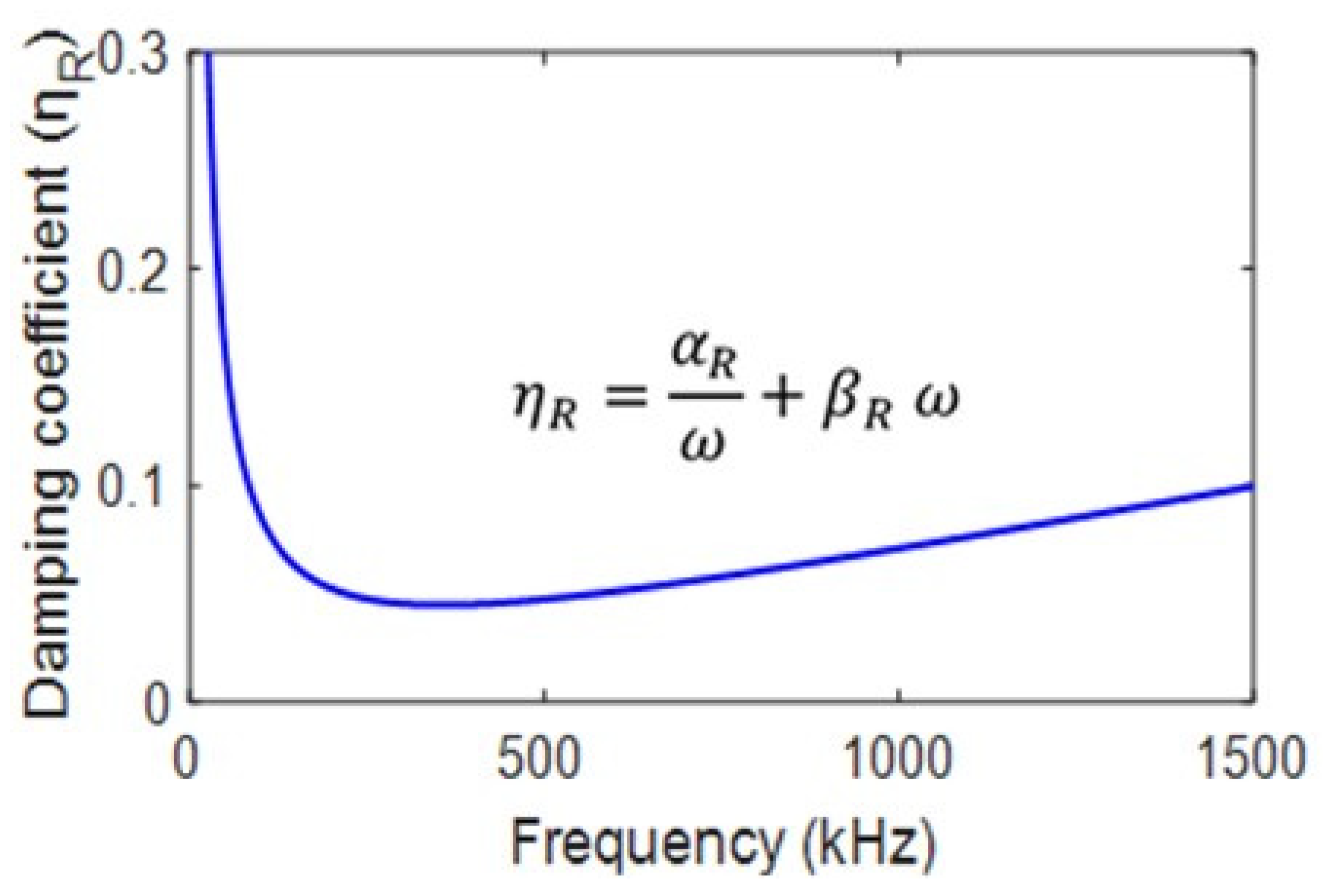
3.3.2. Resonant Sensor

AE sensors cannot transmit all the information of the detected signal, not only because of their sensitivities but also because they transmit the information of the average velocity over the surface in contact [56]. Sensor effect was considered with the same procedure described in [51], summarized hereafter. The resonant sensors were considered by their transfer function Ssensor, which was experimentally determined by the reciprocity method [44,45]. The velocity vz of axial wave was calculated at nodal locations on the sensor surface. In order to account for the so-called aperture effect, the function k represented the sensitivity of a point on the sensor surface at the distance r from the center of the sensor surface. The function value was 1 (maximum sensitivity) at the center and decreased when moving from the center to the edge [51]. An average axial wave velocity VZ was calculated by Equation (1):
V z ( t ) = 1   k   d x   d y   k . v z ( x , y , t )   d x   d y
  k   d x   d y represents the weighted area of the sensor. The radius for the sensors nano 30 was equal to 3.2 mm. The out-of-plane velocity corresponding to the sensor surface contact was calculated and then convoluted with the sensor transfer function following Equation (2):
V s u r f a c e ( ω ) × S s e n s o r ( ω ) = V s e n s o r ( ω )  
where Vsensor is the velocity calculated considering the sensor, Vsurface (ω) represents the mean of out-of-plane velocity on the surface and Ssensor (ω) is the sensor sensitivity function.
The simulated signals were analyzed in time domain and in frequency domain. The main descriptors to be investigated were amplitude or energy, frequency centroid (FC), peak frequency (PF) and the partial powers, denoted PPi. PPi evaluate the frequency distribution in the signal. They represent the percentage of energy contained in separate frequency intervals. For the nano 30 sensor, the intervals were the following, PP1 [0–125 kHz], PP2 [125–250 kHz], PP3 [250–450 kHz] and PP4 [450–1200 kHz]. Additionally, the roll-off frequency was also investigated. The interval [0-froll-off] contained 95% of the energy of the complete spectrum.

4. Results and Discussion

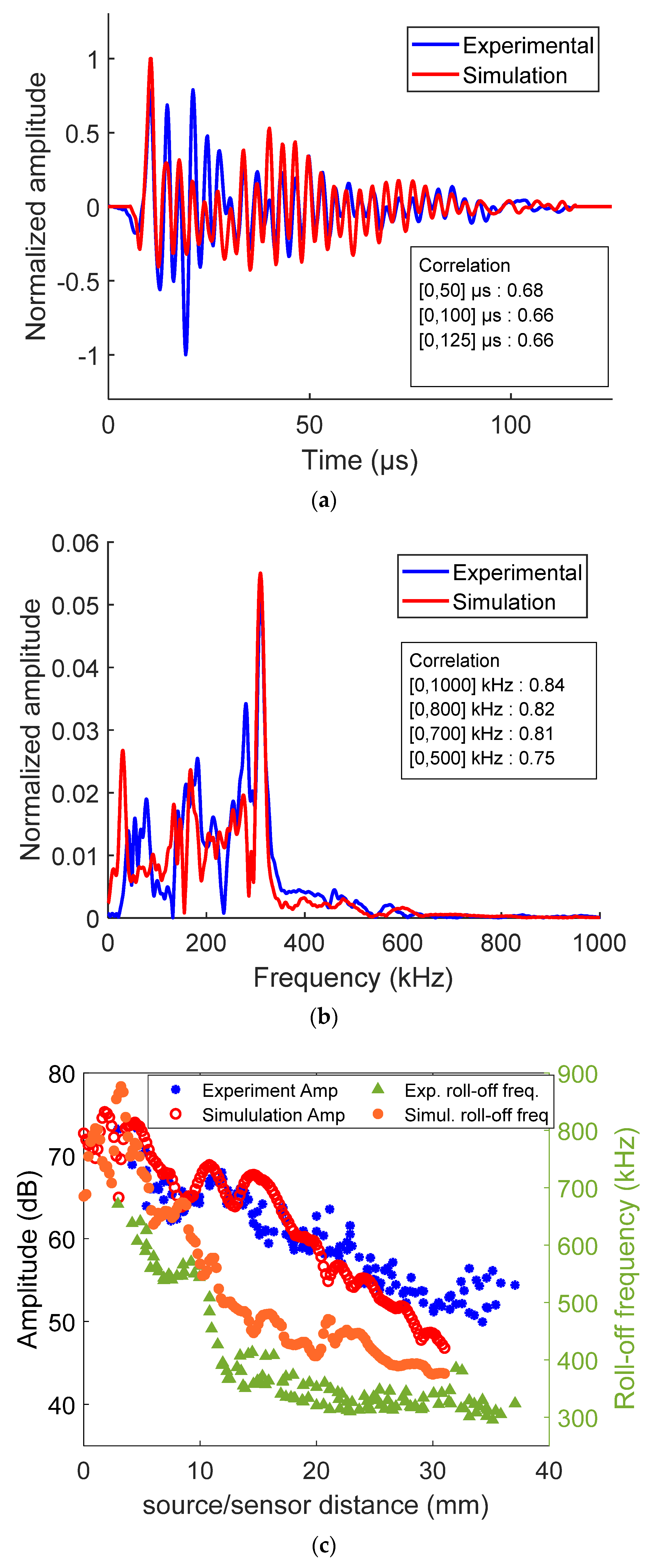
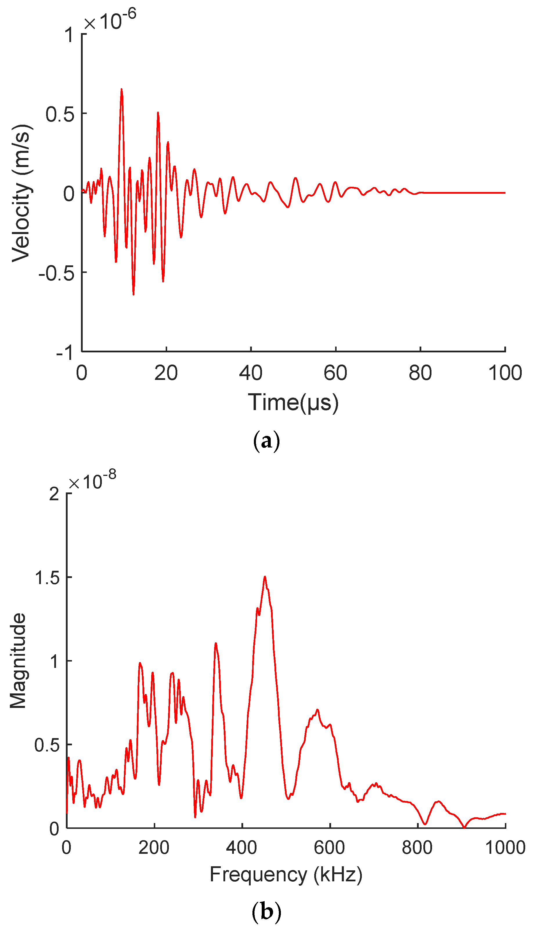
4.1. “Perfect” Signal Due to Validated Simulated Fiber Break

The experimental signals and the simulated signals are presented in order to show the validation of the modeling approach before expanding this numerical investigation to different media and different damage mechanisms. Figure 5a,b shows the direct comparison between experimental signals and simulated signals resulting from fiber break, in time and frequency domains. In this case, sensor C was located 12 mm from the fiber break. Most of the energy of the wave was concentrated below 400 kHz. We could observe a good agreement between the experimental and simulated signals. Figure 5c shows the evolution of two descriptors (amplitude and roll-off frequency) versus the distance of propagation for the experimental data and the simulated data. We also observed a good agreement.
Accordingly, we could use this simulation to extrapolate the signal recorded by a perfect virtual point-contact sensor located at the same position (Figure 6a,b). Contrary to the case with the AE sensor, most of the wave energy was concentrated up to 400 kHz, and the peak frequency was around 500 kHz. Hence, on the surface of the specimen, without the sensor effect, the frequency content was higher. This material surface data, without the sensor effect, could be used to optimize the choice of sensor. The simulation also provided waveforms computed along a straight line on the surface (Figure 2a) in order to further analyze the characteristics of the wave propagation in the medium. Figure 7 shows the results for the 2D-FFT obtained with a virtual perfect point-like contact sensor and with the sensor nano 30 for the simulated data. Even if the identification of the excited modes was not straightforward due to the high number of eigenmodes able to be excited over the studied frequency range, we could observe the F11 bending mode, which could be compared to the well-known A0 antisymmetric mode for an infinite plate. For a specimen of such thickness, in the frequency band of 1 MHz or for a frequency-thickness product up to 2.8 MHz.mm, the source excited a significant number of modes, the predominant ones being bending modes. The 2D-FFT of the signals convoluted by the response of a nano 30 sensor are shown in Figure 7b. When this sensor was used, frequencies above 400 kHz were eliminated. These results clearly show the loss of information related to the choice of sensor. Some of the analyses in the following parts were performed for the perfect virtual point-contact sensor in order to avoid the sensor effect for the parametric studies.

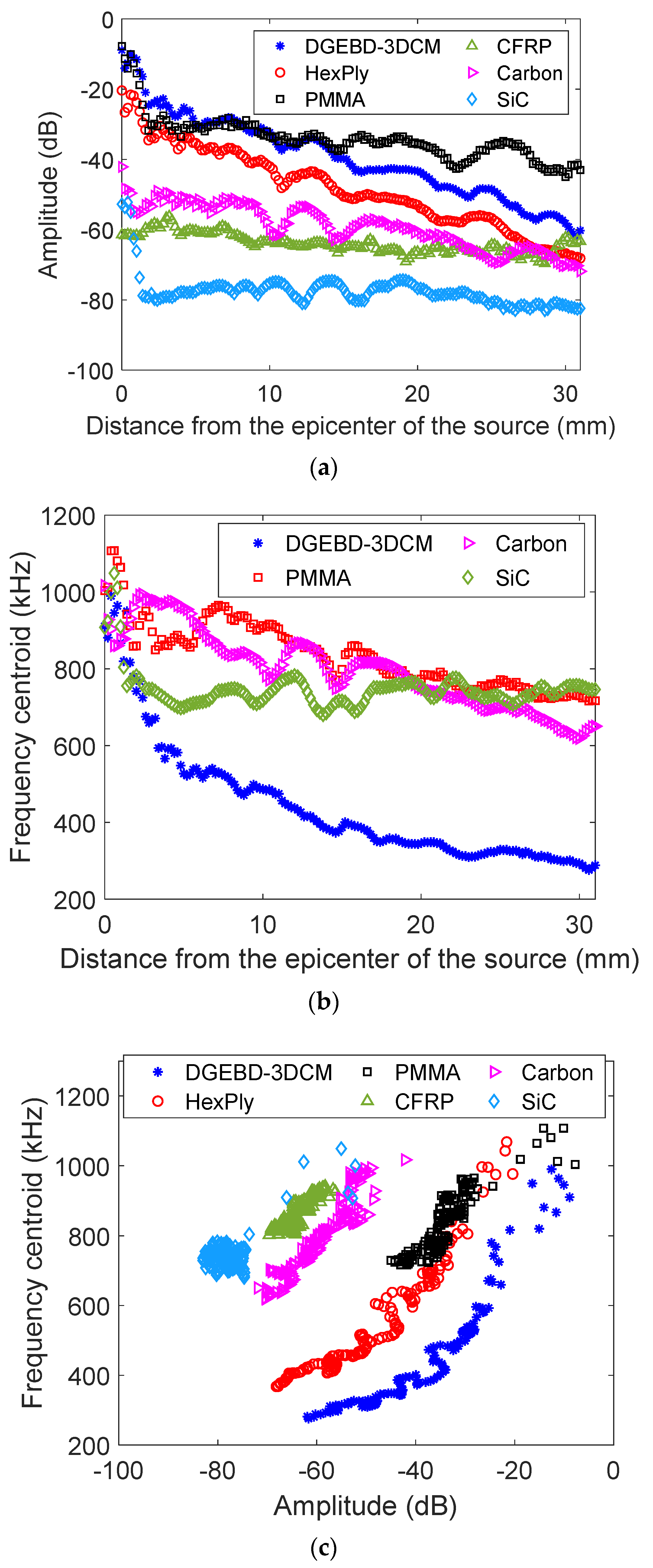
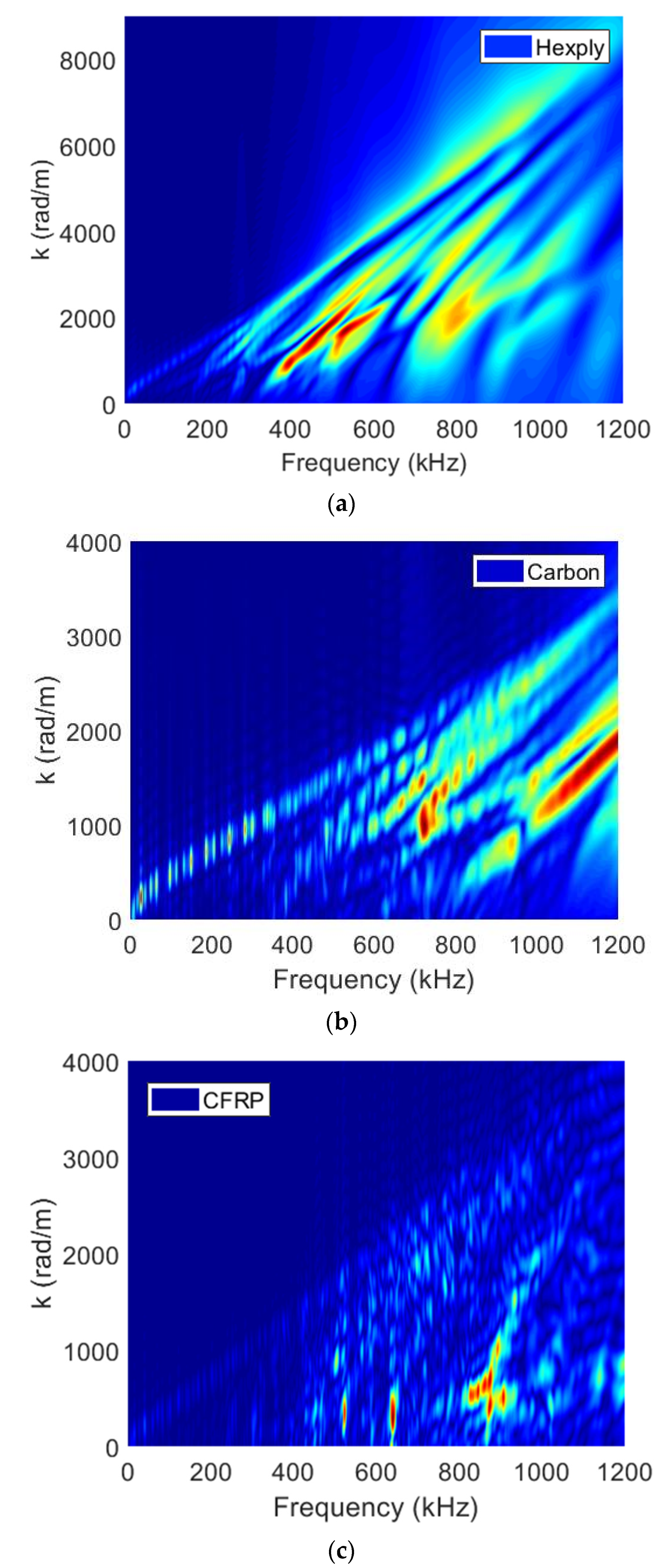
4.2. Influence of the Propagation Medium on AE Signals

In this section, we focus on the influence of the medium around the fiber on the AE signal due to fiber break. As pointed out by Giordano et al. [57], AE parameters such as amplitude or frequency are strongly influenced by the elastic properties of the matrix. For instance, Morscher and Gordon [58] highlighted that fiber break signals could only be detected provided that the sensor is close enough to the damage location, thus evidencing the major influence of the AE propagation medium. The results of fiber break simulations with different matrices are given in Figure 8. The increase in Young’s modulus of the surrounding medium led to a decrease in the recorded amplitude or energy. The signals attributed to polymer media (DGEBD-3DCM, HexPly and PMMA) exhibited higher amplitudes than those obtained for composite or ceramic media. This was due to the high Young’s modulus of the ceramics and the composite, which limited the deformation levels. Even if a perfect point-contact sensor with a flat frequency response was used, the recorded signal reflected the characteristics of the medium rather than those of the source. The mismatch of elastic properties between fiber and matrix strongly affected the AE signal due to fiber break.
For the polymer media, its behavior was characterized by a significant decrease in energy and frequency centroid as the wave propagated through the medium. Higher damping values resulted in more attenuation of high-frequency content, as highlighted in Figure 8b. As a matter of comparison, the frequency recorded by a sensor close to the source was equivalent for all media and hence more accurately represented the source frequency. Figure 8b indicates that the dominant frequency of the source was around 1000 kHz. Due to the viscoelastic nature of the polymer matrix, the AE signals had severe attenuation in high-frequency components. For the ceramic media, the amplitude and the frequency did not change with propagation at this scale. The 2D-FFT obtained with different matrix properties are shown in Figure 9. Plotting the data in the wavenumber/frequency plane allowed the identification of the excited waves obtained for the different media. A strong influence of the elastic properties on the excited waves were observed. Moreover, these representations allowed the identification of parasitic modes due to reflections.
For DGEBD-3DCM and HexPly propagation media, the 2D-FFT showed that the same eigenmodes were excited (Figure 9). For DGEBD-3DCM, the eigenmodes were distributed over a frequency range of [0–800] kHz (Figure 7a), while for HexPly, they were detected in the [0–1200] kHz frequency range. This was due to the material properties that caused the eigenmodes to be excited at higher frequencies. The discontinuity shown in the 2D-FFT of CFRP, carbon and SiC was due to reflections at the edges of the specimen, which disturbed the propagation of the signals. This phenomenon was not observed in the DGEBD-3DCM and HexPly polymers, as the reflections were damped and did not affect the incident signals. The dispersion modes of polymer media were emitted at lower frequencies than those observed for ceramic media. This led to many observed dispersion modes over the studied frequency range in the polymer specimens. For composite or ceramic media, there were fewer excited modes, and they were of higher frequency. The FFT2D of SiC media showed that only two to three modes were excited over the whole frequency range. The acoustic signatures in ceramics were less sensitive to propagation distance, unlike their counterparts in polymer matrices, which were highly dispersive. The viscoelastic nature of the material mainly attenuated the frequencies corresponding to the higher order modes. This consequently affected the content of the signals propagating in the polymer matrix. The energy content of the wave was continuously dissipated. In this case, the propagation distance between AE source and the point of detection had great influence on the frequency content. The representation of the frequency centroid as a function of amplitude (Figure 8c) allowed defining two different groups of materials. We also observed a large scattering of the descriptors for the polymers. This reflected a scattering of the acoustic signature of fiber break in the polymer media in both frequency and amplitude, unlike in the composite and ceramic media where the scattering was less than that of the polymer at this scale. The results obtained with a perfect sensor show that the signature of the carbon fiber break was very different depending on the propagation medium. Moreover, these results show that fiber break did not provide a universal acoustic signature, since the signal emitted by the source was strongly modified by the propagation medium.

4.3. Comparison between Fiber Break and Fiber/Matrix Debonding Signals Computed in DGEBD-3DCM Medium

The results obtained for the instantaneous debonding (Model A) are shown in Figure 10a. The figure shows the evolution of the amplitude as a function of low-frequency content between 0 and 125 kHz for fiber break and fiber/matrix debonding. The data correspond to the signals calculated for different distances d between the source epicenter and the sensor (Figure 2a). In all cases, the amplitude of the signals resulting from debonding was smaller than that of the fiber break even when the debonding size was large (the smallest debonding surface was about eleven times larger than the cross section of the fiber). The AE signal amplitude or energy for the debonding was proportional to its area or to the velocity of the crack. Consequently, higher crack surface areas resulted in higher acoustics emission signal energies for the same conditions of debonding. On the other hand, instantaneous debonding and fiber break admitted similar centroid frequencies. The frequency descriptors showed a frequency content independent of the debonding length (Table 2). Nevertheless, the differences were highlighted. The frequency centroid attributed to the fiber break coincided with that of the debonding up to a propagation distance of 18 mm. Beyond this distance, the frequency centroid of fiber break became slightly weaker. The opening frequency or the partial power in the 0 to 125 kHz frequency range showed a low-frequency content more important in the case of fiber break. Indeed, debonding does not excite the same modes as does fiber break, which excites the fundamental anti-symmetric mode of low frequency. The median value for the frequency centroid for the fiber break was around 370 kHz, whereas the value obtained the fiber/matrix debonding was around 400 kHz.
For a given value of debonding length (L = 100 μm), the energy carried by the wave decreased with increasing source duration or debonding propagation velocity (Figure 10b). Instantaneous debonding in one step corresponded to the highest velocity, whereas the non-uniform progression corresponded to the smallest velocity. The main effect was observed on the energy or amplitude. The energy or the signal amplitude did not only depend on the length of the debonding, but also on the speed of crack propagation and on the kind of damage mechanism. Moreover, the frequency was inversely proportional to the duration of the source. A gradual decrease in frequency content was observed as the source duration increases from 0.1 to 4 μs (Table 2). The frequency content mainly depended on the debonding kinetics rather than on its size. A decrease in the high-frequency content of signals was observed when the debonding velocity was slow. As expected, the highest frequencies corresponded to the signals produced by the fastest source.

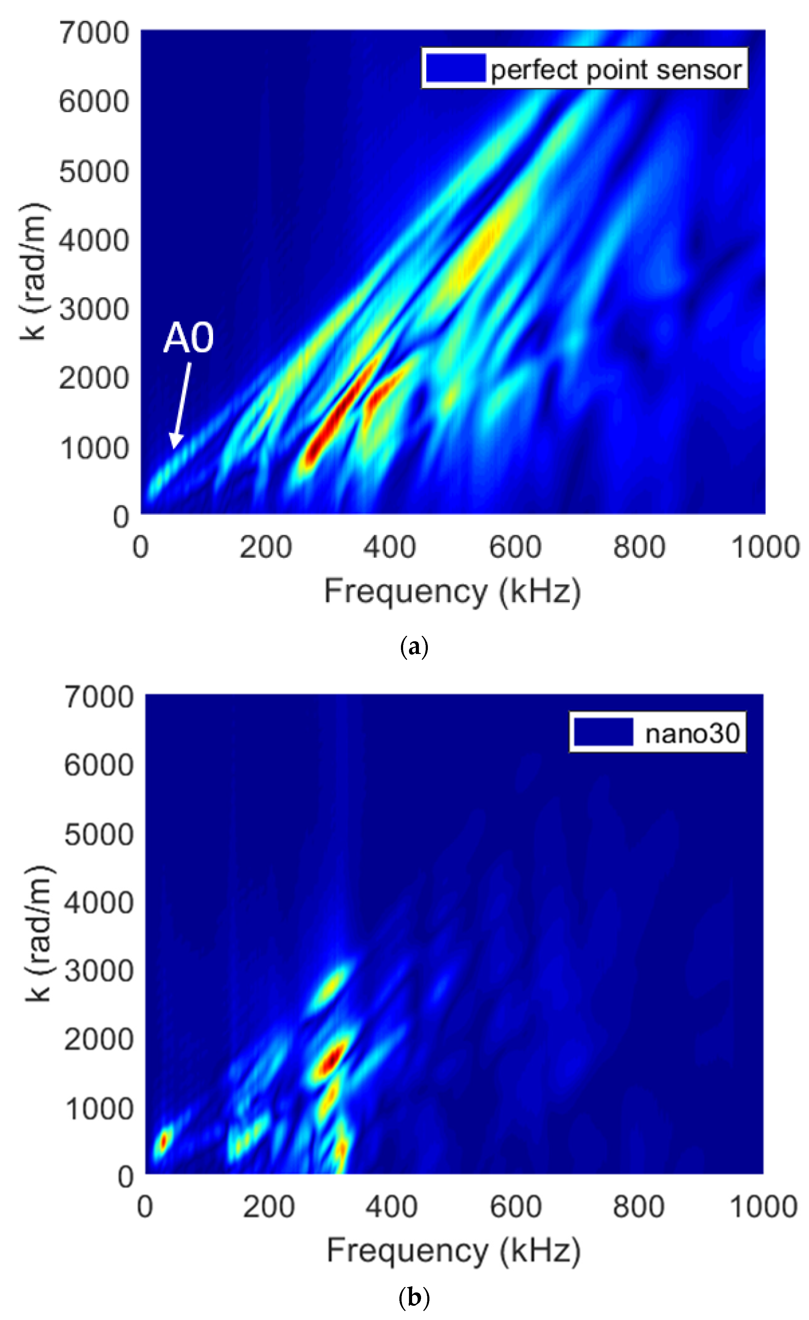
4.4. Sensor Effect and Capability to Detect and Identify the Different Sources

The sensor can bias the signal by filtering certain frequencies. This is of primary importance when designing an experiment, since the signals obtained from a damage mechanism strongly depend on the type of sensor used [17]. The type of sensor can be varied in the simulation and thus give guidelines to which type of sensor and which location on the specimen will be optimal. Figure 11 shows the partial power PP1 in the range of [0–125 kHz] as a function of amplitude for several sources with sensor effect. The signals from fiber break had higher amplitudes than those associated with fiber/matrix debonding (Table 3). The comparison between the results associated with the perfect virtual point sensor and those associated with the nano 30 (Figure 11) shows the remaining differences between the amplitude of the fiber break signals and those associated with debonding. Nevertheless, the response of the sensor reduced the frequency centroid compared to the perfect virtual point sensor for the different debonding configurations and for fiber break (Table 2 and Table 3).
However, we could observe significant changes in the distribution of frequency content (Figure 11b and Table 3). The frequency distribution in the Partial Power PP1 [0–125 kHz] and PP3 [225–450 kHz] domains was different for fiber break and fiber/matrix debonding. The modification was less significant in the range of 125–225 kHz. The signal associated with the fiber contained at least 10% more low frequencies and, on the contrary, the signal associated with debonding had a richer frequency content between 225 and 450 kHz, except for the debonding Model D. The comparison of the values obtained for PP3 and PP1 enabled to discriminate fiber/matrix debonding and fiber break. These results show that in the near field, on the frequency content, it was also possible to differentiate the fiber break from fiber/matrix debonding. Nevertheless, with propagation effects, this difference was blurred beyond 30 mm, making the separation of the mechanisms more complex (Figure 11b). This point is very useful for the classification approaches to increase the robustness of the results.
The data of Table 3 show that for the same debonding length (L = 100 μm) and for Models A and B with instantaneous debonding, the signals had similar values for descriptors (amplitude and frequency). The comparison between Models A and D revealed a significant difference in amplitude and frequency content. This result shows that the debonding condition was a key parameter for acoustic signature.
For the same debonding condition (Model A), debonding length mainly affects the amplitude. Indeed, the comparison between the debonding with Model A for two lengths (20 and 100 μm) showed different amplitudes but similar frequency content.
Moreover, if we assumed a detection threshold of 30 dB, which is often experimentally chosen, the simulation showed a very low detection of 20 μm debonding as well as 100 μm debonding with Model D. On the other hand, for the fiber break for this propagation distance, the detection rate was 100%. For this configuration and material, the signal associated with a 20 μm debonding will not be detected after a propagation of 5 µm, that of 100 μm beyond 25 mm and that of 100 μm Model D beyond 10 mm. All signals associated with debonding will not be detected after a propagation of 25 mm. This result confirms that all the damage mechanisms observed from microscopy may not always be detected depending on the position of the sensor [58]. Numerical simulation of AE offers the ability to evaluate if a damage mechanism occurring in the specimen may be detected by the AE system or not.

5. Conclusions

For a better understanding of the relationship between AE descriptors and a damage mechanism, we have performed a series of AE simulations in a model composite. Indeed, finite element simulations provide a powerful tool for understanding the effect of the source, the medium and sensors on AE signals and descriptors.
The main conclusions without the sensor effect and for the same matrix are the following:
1.
The amplitude of the signals resulting from debonding was much smaller than that from fiber break, even when the size of the debonding was large. On the other hand, instantaneous debonding and fiber break had very similar centroid frequencies.
2.
Debonding also generated high-frequency waves but did not excite the same modes as did fiber break in the near field. Fiber break rather excited the fundamental antisymmetric mode at low frequencies. Nevertheless, this difference in the frequency distribution smeared out with propagation distance.
In near field with the sensor effect, it was possible to easily separate fiber break and debonding signals for a limited propagation distance.
3.
The acoustic signature for debonding was mostly affected by the debonding conditions (instantaneous debonding or progressive debonding). The signals obtained with progressive debonding had lower amplitude and frequency. For instantaneous debonding for different lengths, the amplitude was affected more than the frequency content. The effect of debonding conditions suggests that the use of a mechanical model of debonding would be more suitable for future work.
The effects of the medium on the AE signature of a fiber break are summarized below:
4.
The dispersion modes depend on the mechanical properties of the matrix (Young’s modulus, density, etc.). The dispersion modes detected in polymer materials were much more numerous than in a ceramic material over the same frequency range up to 1 MHz. The viscoelastic nature of polymer materials significantly attenuated the frequency compared to ceramic materials. Young’s modulus plays an important role in the energy content of the signals. The higher the Young’s modulus, the lower the energy content of the signals is. This simulation confirmed the impossibility to obtain a universal signature for the same fiber break in several media. Our study shows that it is not possible to generalize the results of a fiber break signature (amplitude and frequency content) to all composite materials. Therefore, it is necessary to treat each medium independently.
The combination of the sensor effect and the acquisition threshold makes it possible to define the detectability of the source according to its nature and size. After classification of signals, the labeling of each cluster must rely not only on the microscopic observation of damage mechanisms but also on the simulation results of damage due to sources of different sizes and nature. The notion of detectability of the source is rarely considered for the labeling of clusters.
Moreover, AE simulations could provide substantial data for machine learning to increase the robustness of supervised classification. These validated results open the way to combine the experimental and the simulated data to generate a library in order to identify real-time damage mechanisms.

Author Contributions

Conceptualization Z.H., N.G., C.F., T.M. and A.D.; data curation Z.H.; formal analysis Z.H.; investigation Z.H.; methodology Z.H., C.F., N.G., T.M. and A.D.; supervision N.G., C.F., T.M. and A.D.; writing N.G., C.F. and A.D. All authors have read and agreed to the published version of the manuscript.

Funding

This research received no external funding.

Institutional Review Board Statement

Not applicable.

Informed Consent Statement

Not applicable.

Conflicts of Interest

The authors declare no conflict of interests.

References

  1. Eleftheroglou, N.; Zarouchas, D.; Benedictus, R. An adaptive probabilistic data-driven methodology for prognosis of the fatigue life of composite structures. Compos. Struct. 2020, 245, 112386. [Google Scholar] [CrossRef]
  2. Godin, N.; Reynaud, P.; R’Mili, M.; Fantozzi, G. Identification of a Critical Time with Acoustic Emission Monitoring during Static Fatigue Tests on Ceramic Matrix Composites: Towards Lifetime Prediction. Appl. Sci. 2016, 6, 43. [Google Scholar] [CrossRef] [Green Version]
  3. Sause, M. In Situ Monitoring of Fiber-Reinforced Composites: Theory, Basic Concepts, Methods, and Applications; Springer Series in Materials Science; Springer: Berlin/Heidelberg, Germany, 2016; Volume 242. [Google Scholar]
  4. Godin, N.; Reynaud, P.; Fantozzi, G. Acoustic Emission and Durability of Composites Materials; John Wiley & Sons: Hoboken, NJ, USA, 2018; ISBN 9781786300195. [Google Scholar]
  5. Loutas, T.; Eleftheroglou, N.; Zarouchas, D. A data-driven probabilistic framework towards the in-situ prognostics of fatigue life of composites based on acoustic emission data. Compos. Struct. Compos. Struct. 2017, 161, 522–529. [Google Scholar] [CrossRef]
  6. Sause, M.; Schmitt, S.; Kalafat, S. Failure load prediction for fiber-reinforced composites based on acoustic emission. Compos. Sci. Technol. 2018, 164, 24–33. [Google Scholar] [CrossRef]
  7. Eleftheroglou, N.; Loutas, T. Fatigue damage diagnostics and prognostics of composites utilizing structural health monitoring data and stochastic processes. Struct. Health Monit. 2016, 15, 473–488. [Google Scholar] [CrossRef]
  8. Godin, N.; Reynaud, P.; Fantozzi, G. Contribution of AE analysis in order to evaluate time to failure of ceramic matrix composites. Eng. Fract. Mech. 2019, 210, 452–469. [Google Scholar]
  9. Racle, E.; Godin, N.; Reynaud, P.; Fantozzi, G. Fatigue lifetime of ceramic matrix composites at intermediate temperature by acoustic emission. Materials 2017, 10, 658. [Google Scholar] [CrossRef] [Green Version]
  10. Anastassopoulos, A.; Philippidis, T. Clustering methodology for the evaluation of acoustic emission from composites. J. Acoust. Emiss. 1995, 13, 11–12. [Google Scholar]
  11. Ramasso, E.; Placet, V.; Boubakar, L. Unsupervised consensus clustering of acoustic emission time-series for robust damage sequence estimation in composites. IEEE Trans. Instrum. Meas. 2015, 64, 3297–3307. [Google Scholar] [CrossRef] [Green Version]
  12. Morscher, G.N.; Godin, N. Use of Acoustic Emission for Ceramic Matrix Composites; John Wiley & Sons, Inc.: Hoboken, NJ, USA, 2014; pp. 569–590. [Google Scholar]
  13. Alia, A.; Fantozzi, G.; Godin, N.; Osmani, H.; Reynaud, P. Mechanical behaviour of jute fibre-reinforced polyester composite: Characterisation of damage mechanisms using Acoustic Emission and microstructural observations. J. Compos. Mater. 2019, 53, 3377–3394. [Google Scholar] [CrossRef]
  14. Guel, N.; Hamam, Z.; Godin, N.; Reynaud, P.; Caty, O.; Bouillon, E.; Paillassa, A. Data merging of AE sensors with different frequency resolution for the detection and identification of damage in oxide-based ceramic matrix composites. Materials 2020, 13, 4691. [Google Scholar] [CrossRef] [PubMed]
  15. Marec, A.; Thomas, J.-H.; El Guerjouma, R. Damage characterization of polymer-based composite materials: Multivariable analysis and wavelet transform for clustering acoustic emission data. Mech. Syst. Signal Process. 2008, 22, 1441–1464. [Google Scholar] [CrossRef]
  16. Barile, C.; Casavola, C.; Pappalettera, G.; Paramsamy Kannan, V. Application of different acoustic emission descriptors in damage assessment of fiber reinforced plastics: A comprehensive review. Eng. Fract. Mech. 2020, 235, 107083. [Google Scholar] [CrossRef]
  17. Godin, N.; Reynaud, P.; Fantozzi, G. Challenges and limitations in the identification of acoustic emission signature of damage mechanisms in composites materials. Appl. Sci. 2018, 8, 1267. [Google Scholar] [CrossRef] [Green Version]
  18. Kharrat, M.; Placet, V.; Ramasso, E.; Boubakar, L. Influence of damage accumulation under fatigue loading on the AE-based health assessment of composite material: Wave distortion and AE-features evolution as a function of damage level. Compos. Part A Appl. Sci. Manuf. 2018, 109, 615–627. [Google Scholar] [CrossRef]
  19. Carpinteri, A.; Lacidogna, G.; Accornero, F.; Mpalaskas, A.C.; Matikas, T.E.; Aggelis, D.G. Influence of damage in the acoustic emission parameters. Cem. Concr. Compos. 2013, 44, 9–16. [Google Scholar] [CrossRef]
  20. Maillet, E.; Baker, C.; Morscher, G.N.; Pujar Vijay, V.; Lemanski, J.R. Feasibility and limitations of damage identification in composite materials using acoustic emission. Compos. Part A 2015, 75, 77–83. [Google Scholar] [CrossRef]
  21. Oz, F.E.; Ersoy, N.; Lomov, S.V. Do high frequency acoustic emission events always represent fiber failure in CFRP laminates? Compos. Part A Appl. Sci. Manuf. 2017, 103, 230–235. [Google Scholar] [CrossRef]
  22. Aggelis, D.; Shiotani, T.; Papacharalampopoulos, A.; Polyzos, D. The influence of propagation path on elastic waves as measured by acoustic emission parameters. Struct. Health Monit. 2011, 11, 359–366. [Google Scholar] [CrossRef]
  23. Aggelis, D.G.; Matikas, T. Effect of plate wave dispersion on the acoustic emission parameters in metals. Comput. Struct. 2012, 98–99, 17–22. [Google Scholar] [CrossRef]
  24. Al-Jumaili, S.; Holford, K.; Eaton, M.; Pullin, R. Parameter Correction Technique (PCT): A novel method for acoustic emission characterisation in large-scale composites. Compos. Part B Eng. 2015, 75, 336–344. [Google Scholar] [CrossRef]
  25. Dietzhausen, H.; Dong, M.; Schmauder, S. Numerical simulation of acoustic emission in fiber reinforced polymers. Comput. Mater. Sci. 1998, 13, 23–30. [Google Scholar] [CrossRef]
  26. Prosser, W.H.; Hamstad, M.A.; Gary, J.; O’Gallagher, A. Finite Element and Plate Theory Modeling of Acoustic Emission Waveforms. J. Nondestruct. Eval. 1999, 18, 83–90. [Google Scholar] [CrossRef]
  27. Sause, M.G.; Richler, S. Finite element modelling of cracks as acoustic emission sources. J. Nondestruct. Eval. 2015, 34, 4. [Google Scholar] [CrossRef] [Green Version]
  28. Hamstad, M.A.; O’Gallagher, A.; Gary, J. Modeling of Buried Acoustic Emission Monopole and Dipole Sources with a Finite Element Technique. J. Acoust. Emiss. 1999, 17, 97–110. [Google Scholar]
  29. Scruby, C.; Wadley, H.; Hill, J. Dynamic elastic displacements at the surface of an elastic half-space due to defect sources. J. Phys. D-Appl. Phys. 1983, 16, 1069–1083. [Google Scholar] [CrossRef]
  30. Ohtsu, M.; Ono, K. A generalized theory of acoustic emission and source representations of acoustic emission. J. Acoust. Emiss. 1986, 5, 124–133. [Google Scholar]
  31. Ben Khalifa, W.; Jezzine, K.; Hello, G.; Grondel, S. Analytical modelling of acoustic emission from buried or surface-breaking cracks under stress. J. Phys. Conf. Ser. 2012, 353, 012016. [Google Scholar] [CrossRef]
  32. Le Gall, T.; Monnier, T.; Fusco, C.; Godin, N.; Hebaz, S.E. Towards quantitative acoustic emission by finite element modelling: Contribution of modal analysis and identification of pertinent descriptors. Appl. Sci. 2018, 8, 2557. [Google Scholar] [CrossRef] [Green Version]
  33. Sause, M.G.R.; Horn, S. Simulation of acoustic emission in planar carbon fiber reinforced plastic specimens. J. Nondestruct. Eval. 2010, 29, 123–142. [Google Scholar] [CrossRef]
  34. Hamstad, M.; O’Gallagher, A.; Gary, J. Effects of lateral plate dimensions on acoustic emission signals from dipole sources. J. Acoust. Emiss. 2001, 19, 258–274. [Google Scholar]
  35. Wilcox, P.; Lee, C.; Scholey, J.; Friswell, M.I.; Winsom, M.; Drinkwater, B. Progress Towards a Forward Model of the Complete Acoustic Emission Process. Adv. Mater. Res. 2006, 13–14, 69–76. [Google Scholar] [CrossRef]
  36. Cuadra, J.; Vanniamparambil, P.; Servansky, D.; Bartoli, I.; Kontsos, A. Acoustic emission source modeling using a data-driven approach. J. Sound Vib. 2015, 341, 222–236. [Google Scholar] [CrossRef]
  37. Moser, F.; Jacobs, L.J.; Qu, J. Modeling elastic wave propagation in waveguides with the finite element method. NDT E Int. 1999, 32, 225–234. [Google Scholar] [CrossRef]
  38. Åberg, M. Numerical modeling of acoustic emission in laminated tensile test specimens. Int. J. Solids Struct. 2001, 38, 6643–6663. [Google Scholar] [CrossRef]
  39. Burks, B.; Kumosa, M. A modal acoustic emission signal classification scheme derived from finite element simulation. Int. J. Damage Mech. 2014, 23, 43–62. [Google Scholar] [CrossRef]
  40. Suzuki, H.; Takemoto, M.; Ono, K. The fracture dynamics in a dissipative glass-fiber/epoxy model composite with the AE source simulation analysis. J. Acoust. Emiss. 1996, 14, 35–50. [Google Scholar]
  41. Sause, M.G.R.; Hamstad, M.A. Sensors and Actuators, Numerical modeling of existing acoustic emission sensor absolute calibration approaches. Sens. Actuators A Phys. 2018, 269, 294–307. [Google Scholar] [CrossRef]
  42. Gemmeren, V.; Graf, T.; Dual, J. Modeling the acoustic emissions generated during dynamic fracture under bending. Int. J. Solids Struct. 2020, 203, 84–91. [Google Scholar] [CrossRef]
  43. Giordano, M.; Condelli, L.; Nicolais, L. Acoustic emission wave propagation in a viscoelastic plate. Compos. Sci. Technol. 1999, 59, 1735–1743. [Google Scholar] [CrossRef]
  44. Zelenyak, A.M.; Schorer, N.; Sause, M.G.R. Modeling of ultrasonic wave propagation in composite laminates with realistic discontinuity representation. Ultrasonics 2018, 83, 103–113. [Google Scholar] [CrossRef] [PubMed]
  45. Dia, S.; Monnier, T.; Godin, N.; Zhang, F. Primary Calibration of Acoustic Emission Sensors by the Method of Reciprocity, Theoretical and Experimental Considerations. J. Acoust. Emiss. 2012, 30, 152–166. [Google Scholar]
  46. Goujon, L.; Baboux, J.C. Behaviour of acoustic emission sensors using broadband calibration techniques. Meas. Sci. Technol. 2003, 14, 903–908. [Google Scholar] [CrossRef]
  47. Zhang, L.; Yalcinkaya, H.; Ozevim, D. Numerical approach to absolute calibration of piezoelectric acoustic emission sensors using multiphysics simulations. Sens. Actuators A 2017, 256, 12–23. [Google Scholar] [CrossRef] [Green Version]
  48. Cervena, O.; Hora, P. Analysis of the conical piezoelectric acoustic emission transducer. Appl. Comput. Mech. 2008, 2, 13–24. [Google Scholar]
  49. Boulay, N.; Lhémery, A.; Zhang, F. Simulation of the spatial frequency-dependent sensitivities of Acoustic Emission sensors. J. Phys. Conf. Ser. 2018, 1017, 01200816. [Google Scholar] [CrossRef]
  50. Wu, B.S.; McLaskey, G.C. Broadband Calibration of Acoustic Emission and Ultrasonic Sensors from Generalized Ray Theory and Finite Element Models. J. Nondestruct. Eval. 2018, 37, 8. [Google Scholar] [CrossRef]
  51. Hamam, Z.; Godin, N.; Fusco, C.; Monnier, T. Modelling of Acoustic Emission Signals Due to Fiber Break in a Model Composite Carbon/Epoxy: Experimental Validation and Parametric Study. Appl. Sci. 2019, 9, 5124. [Google Scholar] [CrossRef] [Green Version]
  52. Lutz, V.; Duchet-Rumeau, J.; Godin, N.; Smail, F.; Lortie, F.; Gérard, J.F. Ex-PAN carbon fibers vs carbon nanotubes fibers: From conventional epoxy based composites to multiscale composites. Eur. Polym. J. 2018, 106, 9–18. [Google Scholar] [CrossRef]
  53. Bansal, N.P.; Lamon, J. Ceramic Matrix Composites: Materials, Modeling and Technology; John Wiley & Sons: Hoboken, NJ, USA, 2014. [Google Scholar]
  54. Dorvaux-Moevus, M. Mécanismes D’endommagement, Emission Acoustique et DUREES de vie en Fatigue Statique du Composite SiCf/[Si-B-C] aux Températures Intermédiaires (<800 °C). Ph.D. Thesis, University of Lyon, Villeurbanne, France, 2007. [Google Scholar]
  55. Doitrand, A.; Fagiano, C.; Carrère, N.; Chiaruttini, V.; Hirsekorn, M. Damage onset modeling in woven composites based on a coupled stress and energy criterion. Eng. Fract. Mech. 2017, 169, 189–200. [Google Scholar] [CrossRef]
  56. Tsangouri, E.; Aggelis, D.G. The influence of sensor size on acoustic emission waveforms—A numerical study. Appl. Sci. 2018, 8, 168. [Google Scholar] [CrossRef] [Green Version]
  57. Giordano, M.; Calabro, A.; Esposito, C.; D’Aùmore, A.; Nicolais, L. An acoustic-emission characterization of the failure modes in polymer-composite materials. Compos. Sci. Technol. 1998, 58, 1923–1928. [Google Scholar] [CrossRef]
  58. Morscher, G.N.; Gordon, N.A. Acoustic emission and electrical resistance in SiC-based laminate ceramic composites tested under tensile loading. J. Eur. Ceram. Soc. 2017, 37, 3861–3872. [Google Scholar] [CrossRef]
Figure 1. (a) View of the specimen with two sensors C1 and C2. (b) Sensitivity function of nano 30 sensor in reception mode. (c) Axial stress and location of the AE signals localized by the nano 30 sensors as a function of axial strain.
Applsci 11 08406 g001
Figure 2. (a) Location of the simulated fiber break and sensors. The location of the experimental sensor is denoted as C. The fiber break at position P was located 12 mm from the experimental sensor C. (b) Schematic view of fiber break at position P.
Applsci 11 08406 g002
Figure 3. Variation of the damping ratio as a function of frequency according to Rayleigh model for matrix α1 (DGEBD-3DCM).
Applsci 11 08406 g003
Figure 4. Variation of debonding length as a function of time. (a) Model A: instantaneous debonding, (b) Model B: linear progressive debonding (L = 100 μm), (c) Model C: uniform progressive debonding by step (L = 100 μm) and (d) Model D: non uniform progressive debonding by step (L = 100 μm).
Applsci 11 08406 g004
Figure 5. Comparison between simulated and experimental data obtained with nano 30 sensor (a) in time and (b) frequency domains; sensor C was 12 mm away from the fiber break. (c) Amplitude and roll-off frequency vs. source/sensor distance for experimental signals and numerical signals.
Applsci 11 08406 g005
Figure 6. Signal without AE sensor effect in (a) time and (b) frequency domains.
Applsci 11 08406 g006
Figure 7. Simulated dispersion curves (wavenumber k versus frequency f) via 2D-FFT of signals recorded along a straight line for a fiber break at position P on the top surface vz of a computational specimen (e = 2.8 mm and z = 0.9 mm) (a) without sensor effect with the perfect local sensor and (b) with a nano 30 sensor effect.
Applsci 11 08406 g007
Figure 8. Variation of the descriptors (a) amplitude, (b) frequency centroid as a function of the distance between the source fiber break epicenter and perfect sensor location for the simulated signals. (c) Frequency centroid as a function of amplitude.
Applsci 11 08406 g008
Figure 9. Simulated dispersion curves (wavenumber k versus frequency f) via 2D-FFT of fiber break signals recorded along a straight line on the top surface of a numerical specimen (e = 2.8 mm and z = 0.9 mm) without the sensor effect. (a) Matrix α2 (Hexply), (b) Matrix β (carbon) and (c) Matrix γ (composite CFRP).
Applsci 11 08406 g009
Figure 10. Evolution of the Partial Power PP1 [0–125 kHz] vs. amplitude obtained with a perfect sensor for several sources. (a) Fiber break and debonding (L = 20 μm to 200 μm), Model A and (b) fiber break and debonding, Model A, B, C and D (L = 100 μm). The data were calculated from the epicenter of the source to 30 mm of propagation (distance d). V is the velocity of the crack and L is the debonding length.
Applsci 11 08406 g010
Figure 11. (a) Variation of Partial Power PP1 [0–125 kHz] as a function of amplitude obtained with a nano 30 sensor for several sources. The experimental data are also reported. (b) Evolution of PPi (%) as a function of the distance of propagation for fiber break and debonding (Model A, L = 100 μm).
Applsci 11 08406 g011
Table 1. Set of material properties used for FE simulation with three kinds of surrounding medium, matrix type α: polymer medium, matrix type β: ceramic medium, matrix type γ: anisotropic composite medium.
Elastic Modulus (GPa)Poisson’s RatioDensity (kg/m3)Rayleigh Parameter
α R   ( s 1 ) β R   ( s )
FiberCarbon1870.221800--
Matrix type αα1
DGEBD-3DCM
1.410.38103450,000 10 8
Matrix type αα2
Hexply 913 [33]
3.390.35123050,000 10 8
Matrix type αα3
PMMA
[50]
6.20.3211601000 10 10
Matrix type ββ1
Carbone [53]
350.22220010,000 3 × 10 9
Matrix type ββ2
SiC [54]
3500.2315010,000 4 × 10 10
Matrix type γCFRP
[33]
D11 = 147.1; D12 = 4.11
D13 = 4.11; D22 = 10.59
D23 = 3.09; D33 = 10.59
D44 = 3.75; D55 = 5.97
D66 = 5.97
155010,000 6 × 10 10
Table 2. Median values of the descriptors for the data collected by a perfect punctual sensor for different sources. The data were collected from the epicenter of the source up to 30 mm away.
Fiber BreakL = 20 μm Model AL = 100 μm Model AL = 100 μm Model BL = 100 μm Model CL = 100 μm Model D
Frequency centroid (kHz)370400405397339327
Peak
Frequency (kHz)
320365365350294205
Table 3. Median values of the descriptors for the data collected by a nano 30 sensor for different sources. The data were collected from the epicenter of the source up to 30 mm away, without an acquisition threshold.
Amplitude
(dB)
Frequency Centroid
(kHz)
Peak Frequency
(kHz)
PP1
[0–125 kHz]
(%)
PP2
[125–225 kHz]
(%)
PP3
[225–450 kHz]
(%)
PP4
[450–1200 kHz]
(%)
Fiber622372112328427
L = 20 μm
Model A
2128230215235210
L = 100 μm
Model A
4429230613215511
L = 100 μm
Model B
4228829914225310
L = 100 μm
Model C
402622911624546
L = 100 μm
Model D
342261672829367
Publisher’s Note: MDPI stays neutral with regard to jurisdictional claims in published maps and institutional affiliations.

