1. Introduction
Uncontrolled fires pose a significant threat to life and property. Predictions of the evolution of fire are essential for risk assessment and consequence mitigation. However, fires are controlled by complex chemical and physical processes (fluid mechanics, heat transfer, chemical kinetics, solid decomposition, etc.), making detailed predictions difficult, time-consuming and often inaccurate. Furthermore, uncertainty assessment is complex because uncertainties can come from many directions that range from model parameters to the structure and assumptions embedded in the models [
1]. Thermal decomposition of solid materials is one of the processes that are complex to model and carries significant uncertainties.
All aspects of fire growth modeling require some representation of the thermal decomposition of condensed combustible materials. Earlier models relied on simple empirical laws that involved major simplifications and that were mainly based on heat transfer [
2,
3]. A perfect example is the earlier treatment of ignition, where the inert heating approach was used towards establishing ignition criteria. Reviews of these simple ignition models can be found in classic textbooks [
2,
3].
Among the most simplified representations of the onset of combustion are concepts, such as ignition temperatures. By defining such a criterion, the treatment of thermal decomposition is ultimately avoided, and ignition is defined purely as a thermal process [
4]. An empirical determination of an ignition temperature (i.e., the surface temperature at ignition) allows the calculation of parameters, such as the time to ignition, or serves as inputs for simple flame spread models [
2,
3]. More detailed formulations have avoided using an ignition temperature and characterized ignition using a critical mass-loss rate [
2]. Once again, the mass-loss rate is expressed in thermal terms, and these models still do not consider a detailed analysis of thermal decomposition. An empirically determined critical mass flux for ignition serves as the ignition criterion. This ignition criterion has the advantage of using a quantity that can be measured effectively but also provides a direct link with physical concepts, such as flammability limits that an ignition temperature cannot deliver [
3].
The introduction of high-performance computing has made these simplifications unnecessary resulting in the proliferation of many thermal decomposition models that serve as inputs to fire dynamics models [
5,
6,
7,
8,
9]. The objective of these models goes beyond establishing ignition criteria and enables calculating the production of fuel during all stages of a fire. The production of fuel is a key parameter that serves as an input for any combustion model.
Many computational tools have been developed, and each tool has its own specific approach to the modeling of these terms (FireFoam [
5], GPyro [
6], ThermaKin [
7] or Pyropolis [
8]), but a generic representation of the conservation law for fuel is represented by Equation (1):
In this equation represents the mass volume of the solid, the initial mass volume of the solid, the stœchiometric coefficient, is the production rate, the consumption rate and the number of species involved during the degradation process. represents the reactions involving the production of the specie and represents those, which use the species as a reactant. The key to solving Equation (1) is to determine the production and consumption rates.
The first studies are attempting to determine the production and consumption rates, i.e., chemical kinetics, date to the 19th century [
10]. Empirical formulations first emerged, and then they were followed by many authors attempting to use statistical physics theory to justify the form of the empirical laws previously found [
11]. These studies drew a parallel between gas phase and solid phase kinetics. Dating to the middle of the 20th-century, several authors questioned the form of the statistical distributions when applied to the reactions resulting in the thermal degradation of solids [
12,
13].
Among the different approaches, the most common one establishes that for a non-oxidative degradation reaction, the production rate (
) is given by:
where
represents the reaction order,
the pre-exponential factor,
the activation energy,
the perfect gas constant and
the temperature. Then, Equation (2) is composed of the quantity of reactive mass (
) and the reaction rate relation (
). This last relation is known as the Arrhenius relation, first established in 1889 by Arrhenius [
10].
All the current models [
5,
6,
7,
8] have their own representations of the transport equations consistent with conventional conservation equations [
4]. While each author prioritizes specific phenomena relevant to the processes they intend to model, they adopt different simplifications and choose different expressions to model individual phenomena. The same relation (Arrhenius form) is used in all solid degradation models [
13,
14,
15].
Most studies concerned with thermal degradation of solids have not been devoted to formulation itself, but to better understand the input parameters (pre-exponential or the activation energy), to find optimized methodologies to extract these parameters from data, to establish the mechanisms by which fuel is produced and transported (
nth order, diffusion …) and to describe the influence of temperature on the different parameters [
15]. A detailed example of such studies is reference [
16], where it is clearly established that the form of the reaction rate expressions needs to be significantly modified when applied to different materials, many of relevant to fire safety.
It is, therefore, clear that there is great confidence in the capacity of the Arrhenius representation to describe the thermal degradation of solids. Despite this confidence, there is almost no work that serves to unequivocally establish the theoretical underpinnings of the Arrhenius relation. The work of Galwey and Brown [
17] is one the most extensive study devoted to the theory underpinning the Arrhenius relation. While the authors conclude that such a model is inapplicable to the immobilized constituents of a solid, they also indicate that the energy distribution functions at the interface (where reactions occur) are analogous to those in the Maxwell-Boltzmann distribution functions used to justify using Arrhenius for gas-phase reactions. While important, this study focuses on degradation occurring as a single step in an infinitesimally thin interface and, therefore, is not conclusive as support to the wide range of applications of the Arrhenius relation in fire modeling.
Consequently, this article is focused on the Arrhenius relation itself. The objective is to review the basis for the reaction rate relation used for solid degradation and to provide any available justification for selecting any specific form of this formulation. This paper is not intended to prove or disproof the validity of such a relation. Instead, it is directed to organize existing evidence so that those using these expressions in fire modeling can indicate the level of confidence behind the expression.
2. Background of the Arrhenius law
The basic models that represented the reaction rate appeared at the end of the nineteenth century. The modern approach to chemical kinetics due to Wilhelmy, who in 1850 first formulated a kinetic law that described the first-order reaction (see [
11,
18]). This formulation gives a proportionality between the rate of the process and the amount of matter remaining during the sugar cane reaction [
18]. Thereafter, Guldberg and Waage, between 1864 and 1879 [
11], developed the mathematical reaction kinetic expression that was later formalized by Van’t Hoff in 1884 [
19].
After Van’t Hoff, Arrhenius introduced the temperature dependence of the reaction rate and introduced the concept of activation energy in 1889 [
10,
20]. These concepts were then applied to the solid reactions by using the concept of single-step reaction and the introduction of the conversion function (Lewis in 1905 [
21]). After Lewis, the multistep nature of solid-state reactions became increasingly obvious and progressively different complexities have been added to better represent different observed forms of degradation. For more details and explanation of the different empirical approaches and interpretations, the reader can consult references [
11,
18].
However, these approaches are empirical, and none of them brings a theoretical analysis or justification of the Arrhenius relation itself. Although the Arrhenius relation provides good agreement with experimental data, it is not a theoretical justification for the form of the equation.
The next section aims to build from the literature in several domains of physics and chemistry the available information that could serve to provide a theoretical justification for using this kinetic equation in the modeling of solid degradation.
3. Theoretical Approach
The theoretical foundations associated with complex kinetic decomposition models are defined at length scales corresponding to atoms or molecules (≈10
−11–10
−9 m) and typically span time scales defined by atomic motion (≈
or less [
22]). Therefore, the data that is used to support these theoretical foundations must be collected at these time and length scales [
23]. These data are expected to respond to questions required for the assessment of numerous thermodynamic variables [
24].
Many of these variables cannot be resolved when addressing problems that involve larger scales, as will be typical of all fire problems and combustible materials. However, statistical mechanics principles allow the determination of the probability of the occurrence of any particular state in the system. Consequently, if the prediction of the exact behavior of a single molecule is impossible, using statistical methods allows finding the average behavior of an ensemble consisting of many molecules [
25]. Then, statistical averaging is used to increase the scale and reduce the number of variables without losing the necessary molecular-level information. Moreover, finally, this theory is applied to kinetics.
Kinetic laws provide macroscopic representations of the thermal degradation of materials. Nevertheless, they represent phenomena occurring at the atomic level. Statistical thermodynamics provides the tools to bridge the gap between these scales. Therefore, this work begins from the smallest scale and explores the assumptions embedded in the statistical methods used to achieve the macroscopic representation.
3.1. Statistical Mechanics to Describe Energy
At the origin of every transformation, there is energy. The energy stored in any particle (atoms or molecules) can be analyzed using Schrödinger’s equation [
26] and used as a vehicle to provide a physical basis for the upscaling process. The resolution of the Schrödinger’s equation [
25] gives us information about the quantum particles and their state of energy. Thus, the energy of a system is composed of the kinetic energy of each part of the system and the potential energy of all the interactions between all parts of the system.
For a perfect monoatomic gas, the interactions can be considered negligible. Hence the global energy can be described as the sum of the energy of all parts. If the interactions cannot be neglected, then the forces between atoms need to be included in the description of the overall energy of the system. The potential energy of the interactions adds a significant level of complexity. Indeed, in many cases, the interactions are not well-known. If strong interactions exist, then assuming that the global energy of the system is equal to the sum of the energy of all elementary particles (assumption of equipartition) brings uncertainty and potentially significant errors about using the Boltzmann statistics in the Arrhenius equation development. This is an initial and first key assumption that has yet to be demonstrated for materials of the complexity of those involved in fires.
This is a strong assumption, but it enables the description of the energy repartition by the following equation:
Here
represents the total energy of the system,
the level of energy in the state
and
the number of particles in the energetic state
(this definition is consistent with the quantum mechanics definitions, see [
27]). The total number of particles
in all energetic states
is given by:
Based on the previous assumptions, Boltzmann uses statistical mechanics [
25,
28] to develop the path between the microscopic and macroscopic scale (see
Appendix A about the Boltzmann development and the key steps with the Equation (A4) and the Equation (A15), both use the Equations (3) and (4)). To do that, Boltzmann included the configurations and weights of all molecules and all molecule states. Indeed, at any instance, there will be
molecules in the state 0 with energy
and so forth for states 1, 2, etc. (see
Appendix A, Equation (A1)).
To account for the micro-state, in Boltzmann’s statistics, the particles must be identic and distinguishable [
29], here it is mean that the position and the velocity of each particle are known (contrary to quantum particles, for example). This is the second key assumption.
Finally, after an extensive derivation (see
Appendix A), Boltzmann determines the following equation:
Thus, Equation (5) represents the Boltzmann distribution, which describes a number
of particles in the energetic state
. In this equation,
represents the degeneracy of the state
,
is the partition function (see Equation (A12) in
Appendix A),
is the Boltzmann constant and
the temperature [
29].
Equation (5) describes the behavior of an ensemble of particles by a macroscopic expression, and thus the transition between microscopic and macroscopic scale is mathematically formalized.
The Boltzmann equation and its development is the key concept that enables the understanding of the kinetic equation and any potential limitations to it. In the following sections, the main assumptions used in developing Equation (5) are further analyzed to identify other key issues of relevance. These assumptions are then evaluated in the context of the general kinetic law. In doing so, this work extends the study by Galwey and Brown [
17].
3.2. The Formulation of the Arrhenius Form
When considering a reaction at equilibrium in which a reactant
is transformed to a product
(reactants and products can be solids, liquids or gaseous).
A and
B form a system, and this system can, therefore, be described by using Equation (5). The equilibrium constant of the reaction can be expressed as (for more details, see
Appendix B, Equation (A24)):
where
and
are the partition function for
and
, respectively and
is the separation of zero-point energies. In the conversion of molecular energy to molar energy, the constant
is further substituted by the constant
in light of the following relation
where
is the Avogadro number.
This expression serves as a link between Boltzmann’s work (Equation (5)) and the transition state theory (TST). More details and explanations about this development are given in
Appendix A and
Appendix B and in the following references [
27,
30].
The basis of kinetic theory can be found in Wilhelmy, Guldberg and Waage [
11], Van’t Hoff [
19] and Arrhenius [
10]. In parallel to the kinetic theory, developments in statistical physics led to the transition state theory (TST) [
11,
25,
31] and the activated complex theory [
25,
32,
33]. Using transition state theory (TST) as described in [
32], the following well-known expression can be established (see
Appendix B for details):
In this equation, is the kinetic equation (Arrhenius form), is the pre-exponential factor and is the activation energy.
For Williams [
34], the TST approach enables the possibility of describing a greater variety of reactions, including those due to the vibrational mode. Nevertheless, this remains in the context of homogeneous gas-phase reactions consistent with the statistical formulations. The question is now how to interpret the pre-exponential factor (and the partition function, which is part of this factor, (see
Appendix B)) for different types of reactions, in particular those occurring in a solid (ex. reference [
35]).
In gas-phase theory, collision theory was developed in 1916 by Trautz and in 1918 by Lewis [
32,
36,
37] and allows interpreting the kinetic law and its parameters. Subsequently, developing TST allowed Laidler and Glasstone (from 1935) to apply these concepts to a large diversity of reactions [
25,
38], such as:
Elementary reactions in solutions;
Surface reactions, adsorption, chemisorption, etc.;
Gas-phase reactions, single-molecule or multi-molecule.
In all of these cases, each time, these authors found a different form for the pre-exponential factor, but the general expression of Equation (7) remained. Given that the differences can be described through the pre-exponential factor, it is possible to infer that for conventional (chemical reaction) and unconventional applications, the Arrhenius expression is applicable so long the differences are confined to the pre-exponential factor. For this to be the case, the reaction needs to possess an energy barrier. Laidler’s work [
25,
38] well described the transition from a stable state to an activated state. This transition needs a supply of energy called the energy barrier [
25,
38]. Thus, on this basis, Brennan et al. argue the universality of the Arrhenius law [
39]. Further, studies have shown that it is possible to successfully fit a form of the Arrhenius equation to represent the kinetics of any reactions that possess an energy barrier [
40]. It can, therefore, be concluded that it is possible to use these representations of a reaction rate for the reactions involved in the thermal decomposition of a solid despite the absence of a clear theoretical basis.
In solid matter, all the atoms vibrate but stay in fixed, meaning positions because of their strong attractions. Consequently, we assume that the translation and rotation motions do not exist, and their respective partition functions are zeroes. Furthermore, the electrical partition function is also considered negligible because its contribution is considered too low in front of the excited state of the atoms or molecules at an ordinary temperature [
38]. Then, the degradation of molecules is only due to the bond breaks. The bond breaks are the consequence of the high level of vibrational energy.
Finally, for solid reactions, the problem is reduced to vibration inside a solid matrix. This reduction conserves the Arrhenius form Equation (7) and changes the interpretation of the pre-exponential factor, which is only now linked to a vibrational mode. Furthermore, studies by the Eyring [
33], Polanyi and Wigner [
41] and the interpretation provided by Young [
42] indicate that Equation (7) is an appropriate representation of the relevant thermodynamic principles described by Eyring [
33] when only the vibrational mode is considered.
In Equation (7), the activation energy depends on temperature. To simplify the equation, Ellingham’s approximation is frequently used. This approximation indicates that the condition that enables the approximation of to a constant is a negligible standard heat capacity for the reaction.
Through using Equations (6) and (7) (and the detailed development in
Appendix B), it has been shown that the Arrhenius structure can be developed from the Boltzmann distribution for a solid. Nevertheless, the key assumptions that need to be validated when applying this approach include demonstrating a negligible standard heat capacity and the presence of an energy barrier that allows for all the differences to be included within the pre-exponential factor.
4. Applying the Kinetic Model to a Solid Reaction
Often, a good agreement between experimental results and models serves as the only justification for the adequacy of a modeling approach (for example, [
43,
44,
45,
46,
47]). The adequacy of the results can many times be attributed to the way the experimental data are fitted to the model to extract the relevant constants. Indeed, the kinetic models are optimized with data obtained at a scale free of transport processes (≈mg typically TGA scale) and using inverse methods, which can only partially guarantee the good results obtained (for more details about inverse modeling, see [
15,
48]). In the case of fire models, data fits used to optimize kinetic models will be used under conditions that drastically differ from those of instruments, such as a TGA. The extrapolation, therefore, required extreme rigor and a solid theoretical basis.
If a degradation model is necessary to predict fire behavior, and such a model is to be used under conditions that are very different from the experiments used to justify its validity, then using any mathematical formulation for thermal decomposition needs to be adequately justified.
The application of kinetic theory (see
Section 3) in the domain of solid reactions has been the subject of criticism after the 1950s. For example, Paul Garn, through several studies published between 1965 and 1990 about reactions in crystal solids [
12,
49,
50,
51,
52,
53,
54], indicates alternative means of representing decomposition rates. Garn’s main criticism focuses on using the Boltzmann distribution to justify the Arrhenius law for a solid reaction and is argued on the demonstration that this approach leads to a large variety of parameter values found for identical reactions in the literature.
This discrepancy about parameters is partially due to the compensation effect (for details about the compensation effect, see [
55]). Several authors have worked to reduce this source of uncertainties. Furthermore, the ICATC project in 2000 [
56,
57,
58,
59,
60] aims to answer the discrepancy problem by comparing the mathematical methods used with a simple one-step mechanism. After a review of the ICTAC kinetics project in 2009, Dickinson and Heal [
13,
14] conclude about the mathematical functions used (based on the Arrhenius form): “The process is the same as saying that a polynomial equation can be fitted exactly to any data provided a sufficient number of terms is included, and there is not a theoretical meaning to the results.” These authors reach this conclusion because the Arrhenius parameters (see Equation (7) parameters
and
) cannot be found without an optimization process (inverse modeling). Then, these unknown parameters allow a degree of liberty to optimize the model and fit the experimental data well. The recent works of the ICTAC committee [
61] do not change these conclusions. Consequently, Garn’s main criticism remains, and it is not possible to justify the Arrhenius equation with experimental data.
Section 3 shows the importance of the Boltzmann distribution to establish a kinetic law. As postulated in Equation (3), the Boltzmann distribution emerges when no strong interactions between particles can be assumed. By definition, in solids, strong interactions exist. This represents the main fundamental criticism of the Arrhenius form.
Several authors have addressed the issues related to the assumptions embedded in the Boltzmann distribution by using different statistical distributions, for example, by Galwey and Brown [
17]. Some of them have serious doubts about using statistical physics for solid kinetics through the activated approach and want to backtrack to the original work of Van’t Hoff through a thermochemical approach [
62,
63]. However, both approaches have different interpretations of the kinetic parameters, but they are both based upon the Boltzmann statistical theory of energy distribution. Furthermore, Michel [
64,
65] connects the statistical theory for kinetics to thermodynamics through a probabilistic rate theory and solves what the author calls the “inconsistencies of the theories”.
For an overview of the works done in the past 150 years, see [
11,
13,
17,
38,
62,
63,
66]. Attempts to justify the Arrhenius equation for solid kinetic seem to have reached a dead-end, and no one seemed to be able to provide any further evidence to quantify the impact of the interactions between particles on the validity of Equation (3) and the subsequent Boltzmann distribution. In contrast, the evidence of a significant influence of particle interactions was clearly justified by Garn’s [
12] observations on the quantitative discrepancies of the literature values used to represent the kinetic constants for solids. As a result, the common approach to applying the Arrhenius formulation for solids has been its adaptation using additional dependencies. Since the 1950s, several such adaptations of the Arrhenius law for solid applications have appeared in the literature. Examples of such adaptations are the iso-conversional method, the inclusion of a temperature dependency on the pre-exponential factor and the activation energy, etc. Nevertheless, all these studies use the Arrhenius form developed using the Boltzmann statistical distribution. Therefore, they are just empirical interpretations that do not address the key issues explained above.
5. Black Body Radiation to Answer the Problem
A theoretical response to the applicability of the Boltzmann distribution in the Arrhenius relation for the solid degradation based on solid-phase kinetics is clearly not forthcoming. Consequently comes the necessity to investigate the problem from a different perspective.
Reactions within a solid are analogous to radiation in that the vibration of magnetic dipoles (atoms) and hence radiation also depends on the vibrational state of the matter. Planck [
67] postulates a law that enables the representation of radiative heat transfer from a perfect solid (blackbody radiation) [
68,
69]. Planck starts by representing the spectral energy density of radiation by:
Here
represents the spectral energy density as a function of the frequency of the harmonic oscillator (
) and the temperature (
),
is a constant and
is the average energy of the system. In this equation, the quantity
and
must be found. The complete development of Planck’s law is detailed in reference [
68].
To find the average energy
, we have first to describe the repartition of the particles through different energy levels (see [
68]). This description needs micro-statistics and applying Boltzmann statistics, see
Appendix A Equation (A17), leading to the following expression:
Here,
represents the total energy for the energy state
. Considering that,
(see Equation (3)) and that Equation (9) is also used in the kinetic law development (see Equation (5),
Appendix A Equation (A17),
Appendix B Equation (A22)) it can be stated that the kinetic model and radiative transfer model are both based on the Boltzmann distribution (see
Appendix A and [
68]). Here, we have a convergence between the kinetic model and the radiative transfer model.
Finally, according to reference [
68], Planck gives the following expression:
where
is the spectral radiance of a body at absolute temperature
T,
represents the wavelength,
the speed of light,
the Planck constant and
the Boltzmann constant. Equation (10) is called Planck’s law and is largely used for heat transfer by radiation. Furthermore, integrating Planck’s law leads to the Stefan–Boltzmann law (energy
with
the Stephan-Boltzmann constant).
An interesting point in relation to Equation (10) is it uses the same theoretical basis as the Arrhenius equation (see
Appendix B). Therefore, by analogy, the radiative approach allows using Equation (10) to argue the validity of the Boltzmann distribution for solid degradation. Furthermore, Equation (10) is not constituted by unknown parameters or constants that require optimization against experimental data. Consequently, with Planck’s law, the limitations about the Boltzmann distribution use are no longer appropriate.
The previous development made by Planck is accurate for a blackbody, but its application to real materials requires the implementation of some approximations. Indeed, Equation (10) is based on the Boltzmann statistics, such as the Arrhenius equation, then all components of the system (atoms) are considered identic and distinguishable (see
Section 3.1). However, in real materials, all the atoms and the links between these atoms are different. Consequently, some degrees of vibrations (wavelength) are more likely than others. Therefore, it is necessary to contrast a real material to a close to perfect material.
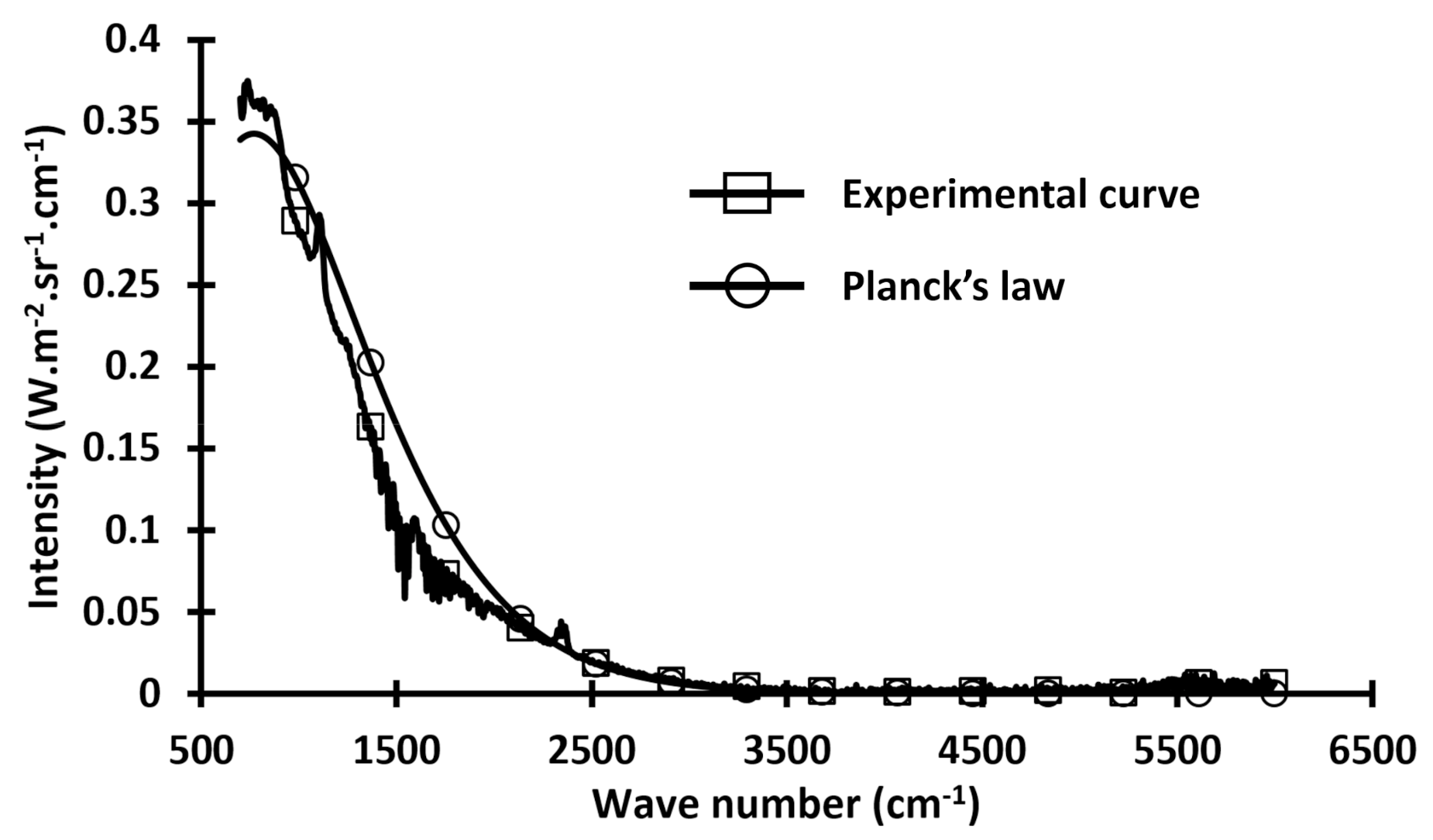
Figure 1 presents the difference between real materials (experimental curve, obtained with a multispectral camera and a wood sample with a black painted surface) and perfect material (curve calculated by Planck’s law for a gray body [
70],
).
Figure 1 illustrates the classical representation of the difference between the gray body model and the real material.
In this figure, the difference between the gray body and the real body highlights the differences introduced by the approximation made by using the Boltzmann distribution in Planck’s law. In
Figure 1, we see that the “real curve” is disturbed, but it follows the gray body model. Consequently, the Boltzmann distribution can be used to approximate the distribution of the vibrational energy through the solid. While this approximation considers all atoms or molecules identic and distinguishable, it provides a trend consistent with real measured values. In a similar manner, it is also clear that there is an error associated with the approximation. Hence, while this approach adds further justification to using the Arrhenius form, it also serves to highlight the importance of adequate means to quantify the errors.
In Equation (10), there are no unknown parameters and no compensation effect contrary to the Arrhenius equation (Equation (7)). Hence, in this section, radiative physics has been used to answer the first problem postulated by Garn [
12] regarding the justification of the statistical distribution of Boltzmann statistics for solid degradation. However, the approach used is valid for elementary reactions, and this approach cannot be used when addressing the large number of elementary reactions involved during the fire-induced degradation process. It is, therefore, clear that partial justification has been achieved, but there are still significant questions left that require the attentive application of this kinetic expression.
6. Conclusions
In this paper, the theoretical underpinnings of the Arrhenius expression are explored, and it has been shown that this expression cannot be fully justified theoretically to be used for thermal degradation of solids, in particular in the case of fires.
The derivation follows using Boltzmann statistics to highlight the main assumptions associated with the theoretical validity of the Arrhenius expression. It was established that for mathematical development, the interactions between molecules must be considered negligible and that the particles must be identical and distinguishable. The validity of these assumptions has yet to be demonstrated for materials of the complexity of those involved in fires. Furthermore, the literature shows ample evidence of deviations from these assumptions.
The analysis of blackbody radiation can be used as an analogy that serves to further justify using the Arrhenius formulation. This approach is free of many of the empiricisms used in solid-phase kinetics; nevertheless, while demonstrating the adequacy of the trends, it also highlights the potential errors associated with using Boltzmann statistics for real materials.
Finally, in the case of fire models, data fits used to optimize kinetic models will be used under conditions that drastically differ from those of instruments, such as a TGA. Therefore, using kinetic models (Arrhenius or alternatives) and their extrapolation requires extreme rigor and a solid theoretical basis.


 ,
, 
