
Genetic Optimization of a Manipulator: Comparison between Straight, Rounded, and Curved Mechanism Links


Department of Robotics, Faculty of Mechanical Engineering, VSB-TU Ostrava, 70800 Ostrava, Czech Republic
*
Author to whom correspondence should be addressed.
Appl. Sci. 2021, 11(6), 2471; https://doi.org/10.3390/app11062471
Submission received: 20 January 2021
/
Revised: 28 February 2021
/
Accepted: 5 March 2021
/
Published: 10 March 2021
(This article belongs to the Special Issue Intelligent Robotics)
Abstract
:There are several ubiquitous kinematic structures that are used in industrial robots, with the most prominent being a six-axis angular structure. However, researchers are experimenting with task-based mechanism synthesis that could provide higher efficiency with custom optimized manipulators. Many studies have focused on finding the most efficient optimization algorithm for task-based robot manipulators. These manipulators, however, are usually optimized from simple modular joints and links, without exploring more elaborate modules. Here, we show that link modules defined by small numbers of parameters have better performance than more complicated ones. We compare four different manipulator link types, namely basic predefined links with fixed dimensions, straight links that can be optimized for different lengths, rounded links, and links with a curvature defined by a Hermite spline. Manipulators are then built from these modules using a genetic algorithm and are optimized for three different tasks. The results demonstrate that manipulators built from simple links not only converge faster, which is expected given the fewer optimized parameters, but also converge on lower cost values.
1. Introduction
The most common serial manipulator design in the industry benefits from its so-called angular structure with 6 degrees of freedom, which can easily reach the surrounding areas and achieve multiple different poses. However, this universal kinematic structure has a disadvantage in that when such robots are deployed in densely built workplaces, they can collide either with obstacles or themselves. Custom manipulator designs can overcome this problem, as best shown in the work by Brandstoetter [1], where he presented a robotic manipulator with a task-desired kinematic structure.
Evolutionary robotics (ER) is often used to create custom robots or their components, such as the morphology, kinematics, or controllers. It is a set of evolutionary techniques used for the development of robotic systems, as stated by Nolfi [2] in his book, which delivered the theoretical basics for this topic. ER strategies were described in a survey by Back [3] and in a newer paper by Li [4]. ER is often used to synthesize robot controllers for a specific behavior [5] or multiple behaviors [6]. One of the use cases for evolutionary robotics is in determining the kinematics required for a robot to optimally perform a task or a set of tasks. The reason for the usage of optimization algorithms is that the synthesis of the kinematic structure of a manipulator is a rather complicated task if an analytical approach is used. One of the recent achievements in terms of analytical manipulator synthesis was the synthesis of three-revolute spatial chain by Hauenstein to allow five poses [7]. Evolutionary robotics can provide satisfying results nowadays, allowing more degrees of freedom and more poses (or even entire trajectories).
The optimization problem is often carried out on kinematic structures built from predefined modules. Hornby [8] was one of the first that demonstrated the possible application of evolutionary robotics in practical engineering work by evolving a design for walking robots. More of these examples can be found in the survey by Alattas [9]. The research on the evolution of manipulators built from adaptive modules to perform desired tasks was started by Han [10], who determined the optimal robot configuration and the length of links between modules. Chocron [11] also found the optimal kinematic structure for the modules that he defined. Another solution was presented by Valsamos et al. [12,13], who presented a more developed approach with so-called pseudo-joints, which with the use of a genetic algorithm (GA) attempts to find the kinematic structure with the best manipulability. Their outcomes were later verified by Katrantzis [14] in an experiment with a real manipulator.
It is important to note that the use of a genetic algorithm is not the only possible approach to solve the presented issue. Patel [15] used a simulated annealing algorithm, while Ha [16] addressed the issue using a heuristic-guided tree search algorithm. Whitman [17] and Dogra [18] applied a deterministic quasi-Newton algorithm to find the local minimum of a cost function.
The complexity of the modules from which a robot is constructed determines the optimization difficulty. In this context, the complexity of a module can be thought of as a number of parameters describing one module and the variety of shapes it can achieve. Liu et al. [19] showed that changing the number and position of connecting faces in a module influences the evolvability of a modular robot. In another study [20], Moreno and Faina used the same robotic modules to show how changing the length of modules affects the resulting robot structures and performance.
The performance of an open-chain manipulator can be improved for a specific task by optimizing the Denawit–Hartenberg (DH) [21] parameters. Ceccarelli optimized the DH parameters of a 3R manipulator for a specific workspace geometry [22]. Singla [23] presented a method for synthesizing serial redundant manipulators by optimizing their DH parameters in an environment with obstacles. Previously studies that have used DH parameters to optimize task-specific manipulators have generally been limited to predefined modules or straight modules with variable lengths. Brandstöter [1] presented a concept of a modular robot with a general kinematic structure and curved links. Unlike these previous studies, we investigate and compare configurable straight and curved links in a single set of motion tasks.
The purpose of this study is to demonstrate how the complexity of modules affects the overall robot kinematics optimization results. We demonstrate this by optimizing a manipulator built from link modules with different complexities for three different tasks. Furthermore, we use two different cost functions and compare how the results differ. First, the simulation of the manipulator, the joints, and the different types of links are described. Then, the optimization process and tasks are described and the results are presented.
2. Materials and Methods
In this study, we tested the performance of different mechanism links for task-specific manipulator optimization.
In this study, we used a genetic algorithm (GA) implemented in .NET C# combined with a simulation implemented in CoppeliaSim [24], whereby the GA takes care of the optimization and the simulation provides a way to evaluate the individuals proposed by the GA and calculates their cost value.
2.1. The Manipulator
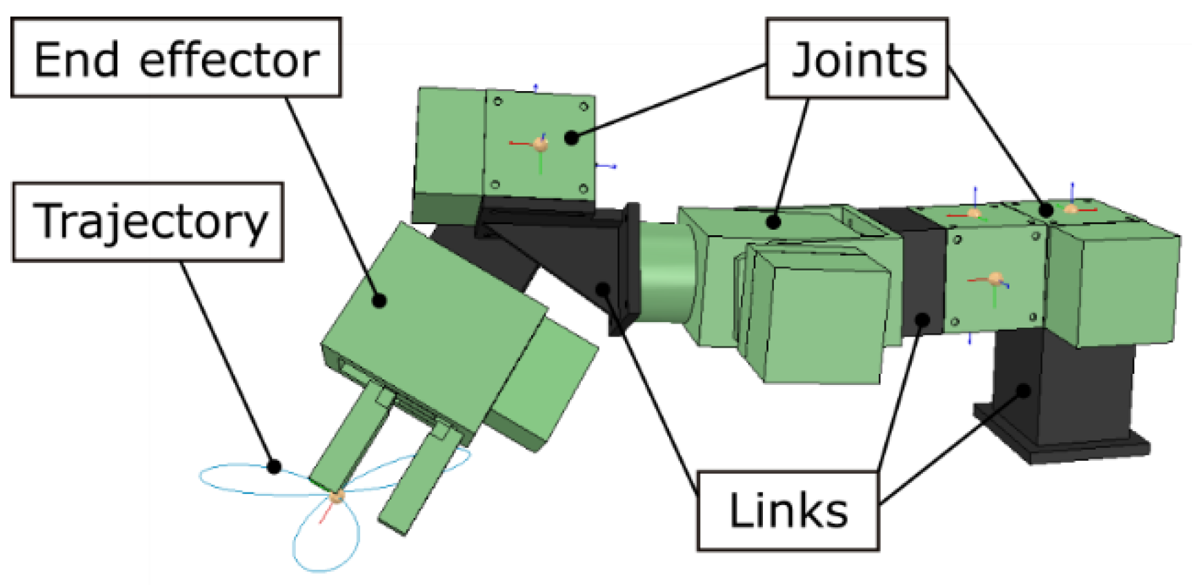
The algorithm uses links, joints, and an end-effector to build a serial manipulator for evaluation. The manipulator always starts with a link, while the placement of links and joints alternates so that there are never two links or two joints connected to each other. The end-effector is connected to the last link or joint. An example of a manipulator built by the algorithm is shown in Figure 1.
2.2. Manipulator Joints
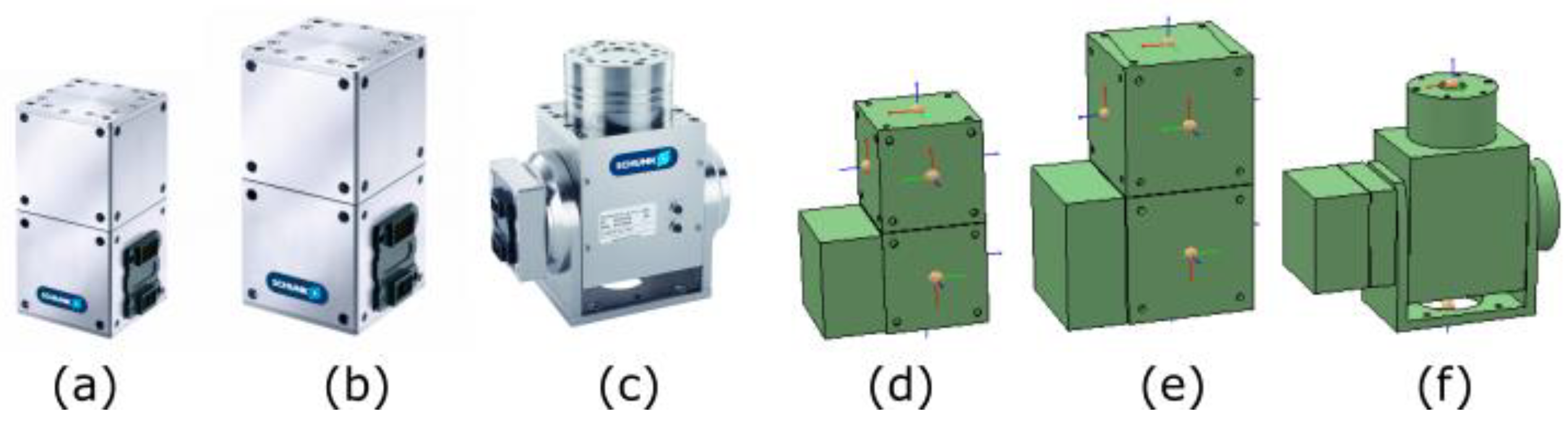
Since we focused on the manipulator links in this paper, we limited the selection of joints to three different modules. All manipulators were built only from those three joint modules (Table 1). We selected joint modules manufactured by Schunk (production models PR70, PR90 and PW70) and created corresponding models (matching in size, weight, inertia, and torque) in CoppeliaSim (Figure 2). For simplicity, only rotational joints were considered. Two of the joint modules contained a single rotational joint and one was a double joint module. The modules can be reused an unlimited number of times, i.e., all joints in a manipulator can be instances of one joint. The joints were implemented in the genetic algorithm as genes comprising three parameters: joint type (ID), orientation between previous link and the joint (ora), and orientation between the joint and the subsequent joint (orb). It is possible to connect the modules using four different orientations, hence the four orientation values separated by 90°. Ranges of the joint parameters are shown in Table 2.
2.3. Manipulator Links
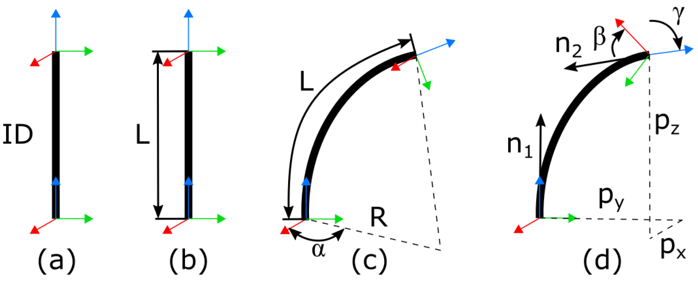
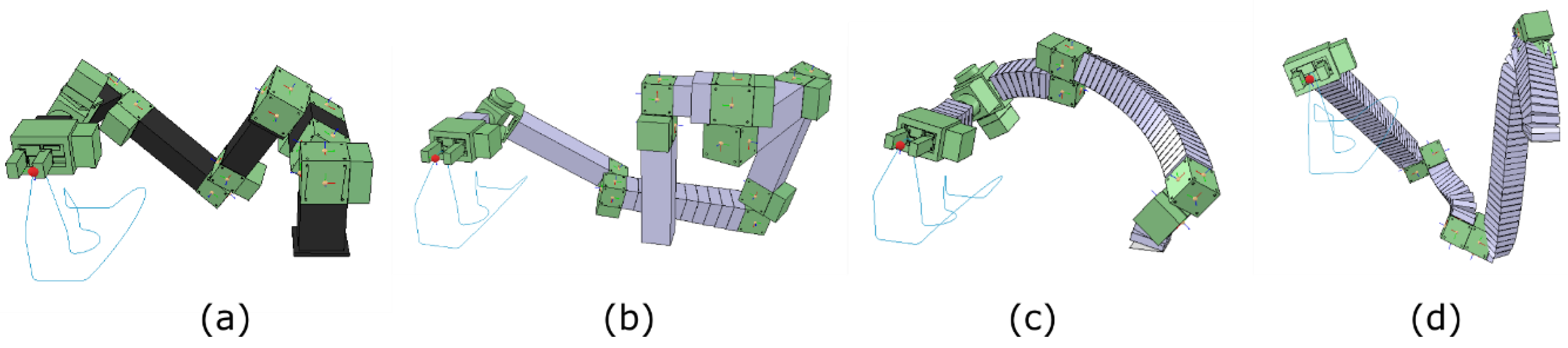
The links of the manipulator were the main focus of this study. There were four different types of links used in this study. Each type of manipulator link is defined by the different parameters listed in Table 3. Each parameter is an integer and is passed to the simulator at initiation. Figure 3 shows the comparison of all link types.
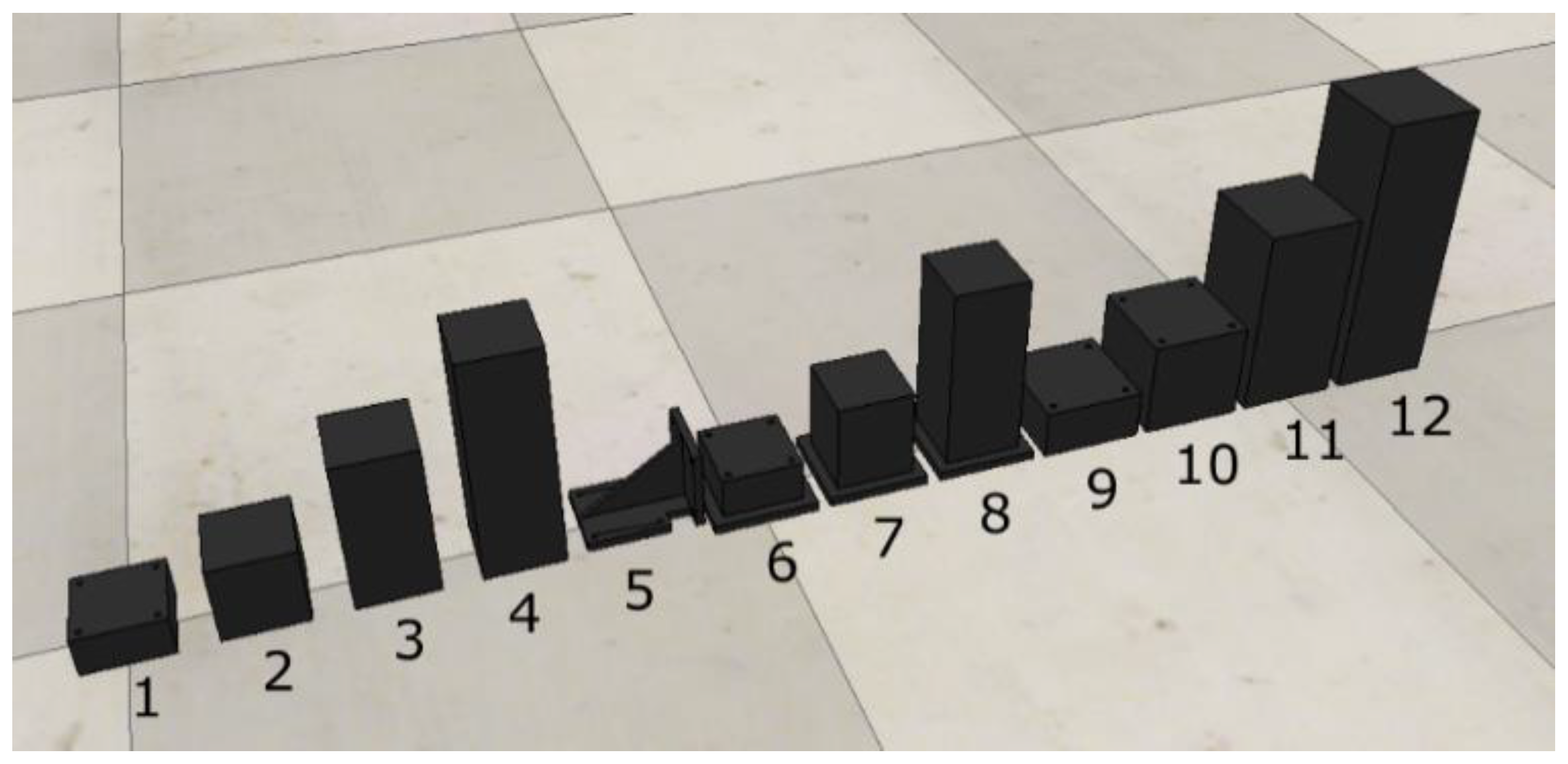
Each link type is built differently. The basic link type is a simple straight link, which is selected from a set of predefined links (Figure 4). The only thing defining which link module to use is a single parameter ID. One of the modules (ID 5) is shaped at 90 degrees to allow for more variability in solutions. Since the joint modules have two available flange sizes (70 and 90 mm), the modules are prepared to end with 70 and 90 mm flanges on one or both sides. Parameters corresponding to the IDs are listed in Table 4.
The linear link type is a straight link of variable length. In this case, there is also only one parameter describing the link module. However, instead of selecting a link with a predefined length, the link is generated according to the length parameter.
The rounded link type is defined by three parameters and has a semicircular shape. This type of link module allows for bends and twists in the links; as such, the joint axes do not have to be orthogonal and unconventional kinematic structures can be achieved.
The Hermite link type is built using a Hermite spline [25]. This allows for even more control over the shape of the link than the other types and should be better suited to avoid self-collisions. The drawback of this type of link is that it is described by 7 parameters, and thus makes the problem computationally demanding for optimization algorithms.
Flange sizes for linear, rounded, and Hermite links are not prepared in advance, as in the case of basic links. Instead, the thickness of the generated link object in the simulation is adjusted accordingly based on the flange size.
These four types of manipulator links extend the commonly used straight links to include rounded and curved links. They also highlight the differences between predefined straight links and straight links with variable length.
2.4. Optimization
The genetic algorithm creates a population of chromosomes. Each chromosome describes one manipulator structure. The chromosome combines links and joints, starting with a link module. Then, the population is simulated. Before each simulation, the chromosome is parsed into CoppeliaSim and a manipulator is built. The simulation starts and measurements are performed for the position and orientation of the end-effector, collisions between modules, and the torque in every joint. These values are used to calculate the cost function, which is the input to our genetic algorithm. After simulating every chromosome in the population, the algorithm sorts the chromosomes according to their calculated cost, performs crossover and mutation, and creates a new generation of chromosomes for testing.
2.4.1. Genetic Algorithm
The optimization algorithm is a basic genetic algorithm with single crossover and mutation operators. We chose to implement a rather simple GA [26], since we were not interested in the performance of the GA itself but rather how the complexity and flexibility of various links perform under the same conditions.
The GA is set to run on a population of 25 chromosomes for 150 generations, while keeping 3 chromosomes in an elite class. The chromosomes or potential solution candidates are selected from the population based off their fitness, or in this case their cost score. They are then subject to crossover and mutation to produce another generation of solutions until the algorithm reaches the maximum generation count. The genetic algorithm is run ten times for each link module type and each trajectory. We then look at the best results from each run and the median of the best results for all runs and compare them.
2.4.2. Crossover and Mutation
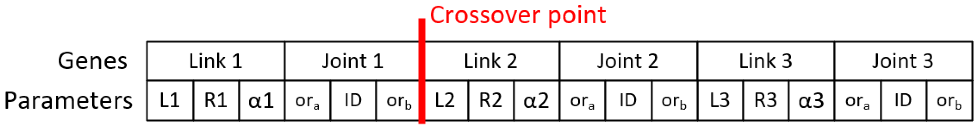
Crossover and mutation are genetic operators that are used to create a new generation of chromosomes (potential solutions for the specified problem). The crossover creates a new child chromosome from parent chromosomes by splitting the parents into parts and assembling the parts to produce a new offspring. The mutation introduces new genetic information into the chromosomes by randomly changing some of their genes. The chromosomes are comprised of link genes and joint genes. We used a single crossover, with the position of the cut located between the genes. Figure 5 shows a chromosome for a manipulator with 3 degrees of freedom built from rounded links (3 parameters per link), with a highlighted crossover point.
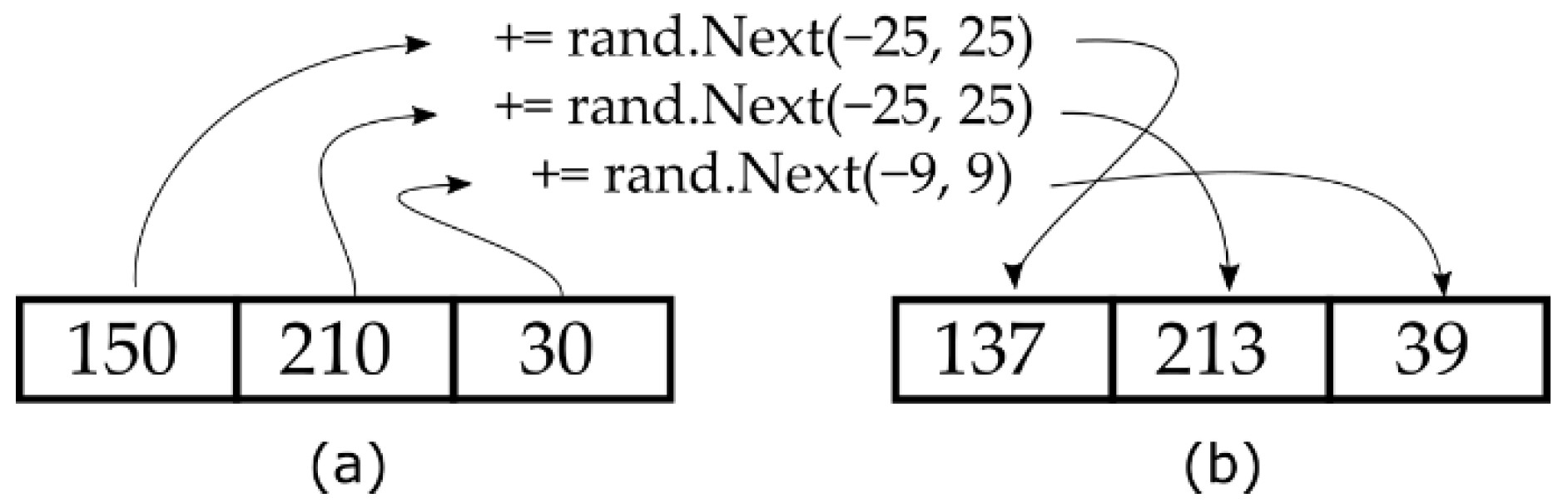
Each link type is implemented in a similar fashion. When the link gene is selected for mutation, it increases or decreases its parameters by a random number. The random number is selected from a range, which is 1/10 of the range for the parameter (Figure 6).
During the mutation of a chromosome, there is a random chance for a gene to be completely deleted or a new gene to be inserted into the chromosome. This allows the algorithm to change the number of degrees of freedom of the manipulator.
2.4.3. Cost Functions
In this article, we describe tests with two different cost functions: cost1 and cost2 Value cost1 is defined as a weighted sum of the end-effector position, orientation errors, and manipulator collisions (Equation (1)). Function for cost2 is adapted from the cost1 and torque measurements are added (Equation (2)). The weights are handpicked so as to put the members of the equation into the same range:
where col is a measure of collisions, εpos is the sum of positional errors, εori are the errors in orientation, wpos is weight of the position part of the cost function, and wori is weight of the orientation part:
where cost1 is calculated according to Equation (1), the Tsum is a sum of torque measurements for each joint during the simulation, and wT is the weight of the torque part of the equation.
The detection and measurement of collisions, positions, and orientation errors and torques are described in the following chapters.
2.4.4. Detecting Collisions
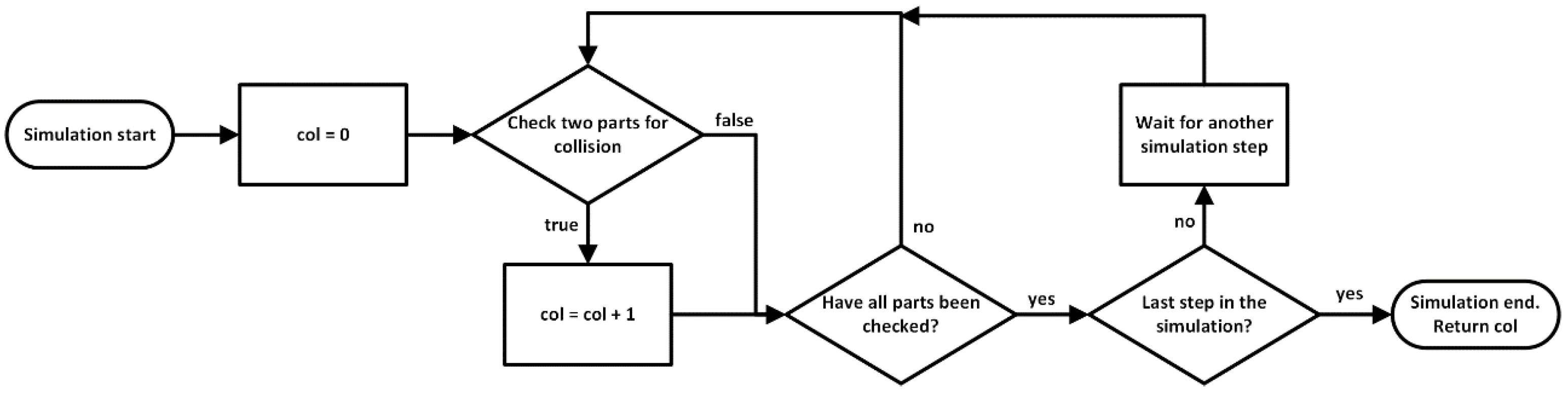
To increase the number of viable solutions, we checked for collisions between individual parts of the manipulator. The script for checking collisions was implemented in CoppeliaSim and uses a built-in function that checks for collisions between two objects. This function takes two objects in the simulation scene as parameters and returns a true result if there is a collision between them, i.e., the two parts are overlapping. In this way we detected collisions between all objects and incremented a collision count each time two objects collided (Figure 7). The script returns a value marked as “col”. This collision check is done at each simulation step (50 ms). Therefore, if some parts collided for only a short amount of time, the resulting “col” value will be a smaller number.
The objects that form the manipulator are allowed to pass through one another and their collisions are measured. Disabling dynamic interactions between objects helps to avoid local minima during optimization.
The collisions are counted inside the script in CoppeliaSim and the result is parsed to the C# program at the end of the simulation. A potential hurdle in this method could be the indifference between two parts touching or directly passing through one another.
2.4.5. Position and Orientation Errors
The end-effector of the manipulator has a coordinate system (CS) placed inside the gripper. There is a target CS that moves along the task trajectory during the simulation. Inverse kinematics in CoppeliaSim are set up so that the CS of gripper follows the target CS. Depending on the simulated manipulator, the inverse kinematics are either able or unable to converge to the target CS and errors in position and orientation may occur. The errors are measured at each simulation step and summed according to the following Equations (3) and (4):
where i is a simulation step; n is a total number of simulation steps; xef, yef, and zef are coordinates of the end-effector; xtar, ytar, and ztar are coordinates of the target; αrel, βrel, and γrel stand for the relative orientations between the end-effector and the target coordinate frames.
2.4.6. Torque Measurements
The torque on each joint is measured at every simulation step and the results are summed (Equation (5)). This torque sum is then used to calculate cost2. Measuring the torque as a sum of all joint torques should make the algorithm prefer lighter manipulators with lower energy consumption:
where i is a simulation step, n is the total number of simulation steps, j is a joint, k is the total number of joints in a manipulator, and Tj is a torque measurement for joint j.
2.4.7. Tasks
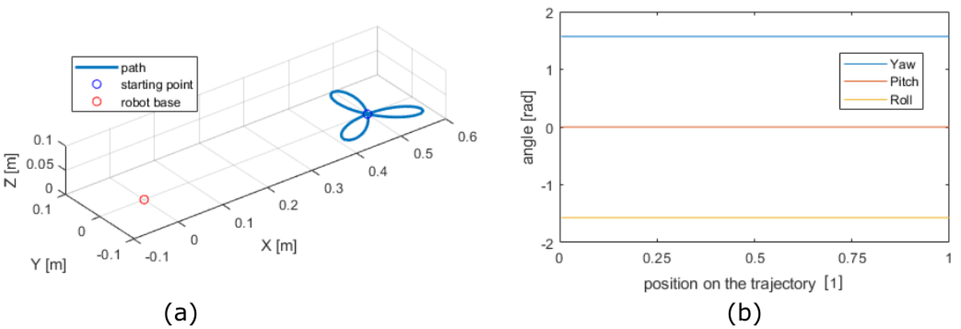
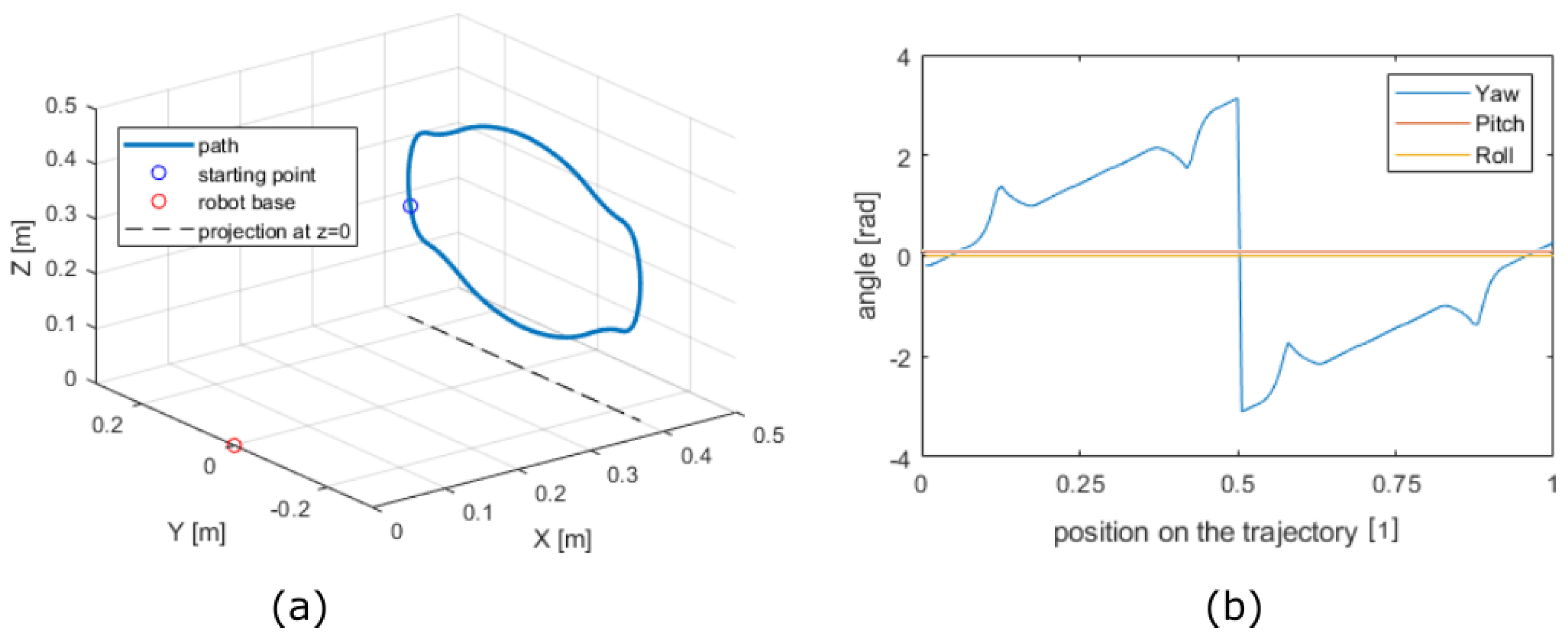
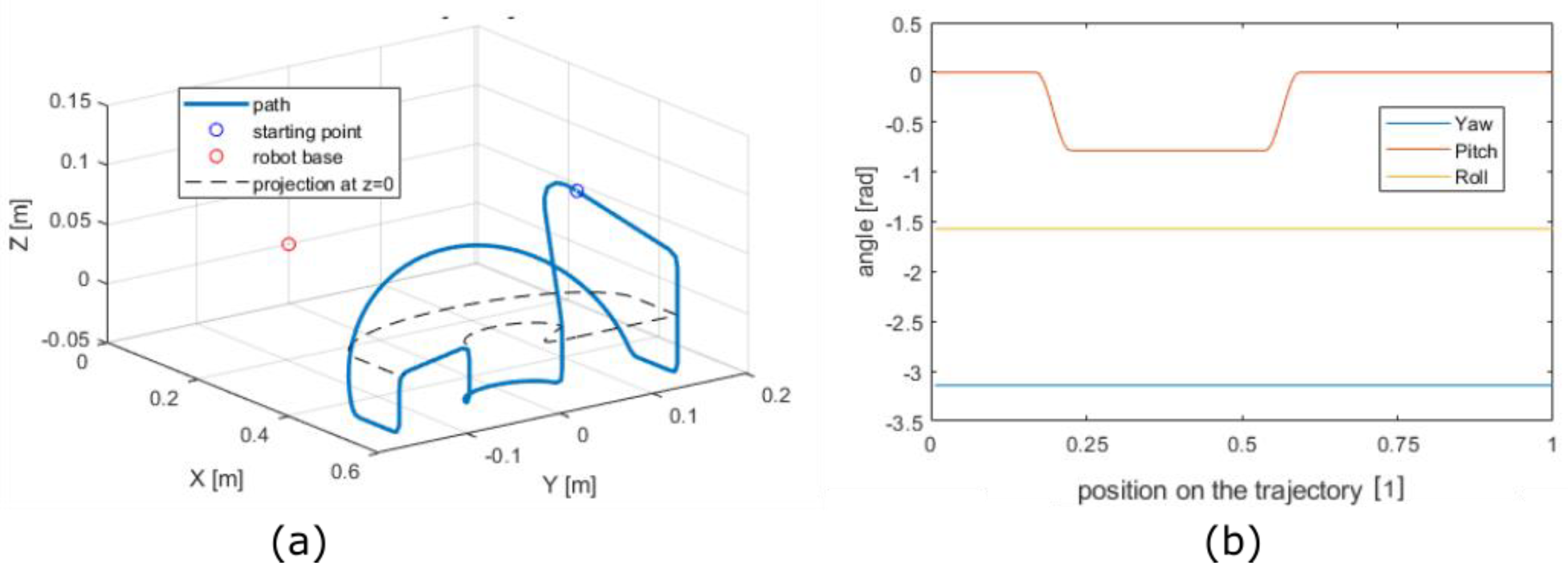
We tested the algorithm on three different tasks. In all three cases, the robots’ base was positioned at the origin of the coordinate system. Each task is described by a trajectory that is placed approximately 0.5 m in the direction of the X axis. The trajectories are defined as 6D curves, e.g., each point on the curve has 3 positional degrees of freedom (DOF) and 3 DOF in orientation. Task 1 (Figure 8) is a trajectory formed by a curve of the fourth degree called trifolium. This curve was used by Brandstöter [27] to optimize positional error on a modular manipulator. The curve lies in the horizontal plane and the orientation does not change throughout the whole trajectory. Task 2 (Figure 9) simulates a welding task, where the end tool of the robot needs to traverse a rounded trajectory with changing orientation. The trajectory is in the vertical plane, with the normal oriented towards the robot base. In this case, the orientation changes in one axis along the whole trajectory. Task 3 (Figure 10) was created to provide the manipulators with a difficult trajectory. It is formed by connecting several curves together. It curves in all directions and passes above and below the robots’ base. The horizontal axis in the orientation plot is a position parameter, which goes from 0 to 1 and corresponds to the start and end of the trajectory.
In real applications, in addition to the position and orientation, the description of a task would also include other motion data, such as the motion type, speed, and zones. In our simulations, we simplified the tasks to have a constant speed of 0.25 m/s. The points on the trajectory have no specified zones for corner paths or defined position accuracies. The generated robot attempts to follow the path as precisely as possible and the position and orientation errors are measured.
3. Results
The optimization procedure was run ten times for all combinations of the 3 trajectories, 4 link types, and 2 fitness functions. In total, 240 runs of the genetic algorithm were performed. Each run took approximately 2 h on a mid-range PC (Intel® i7-7700HQ, 16 GM ram, Nvidia GTX 1060), so we had to divide the work across several computers and multiple days.
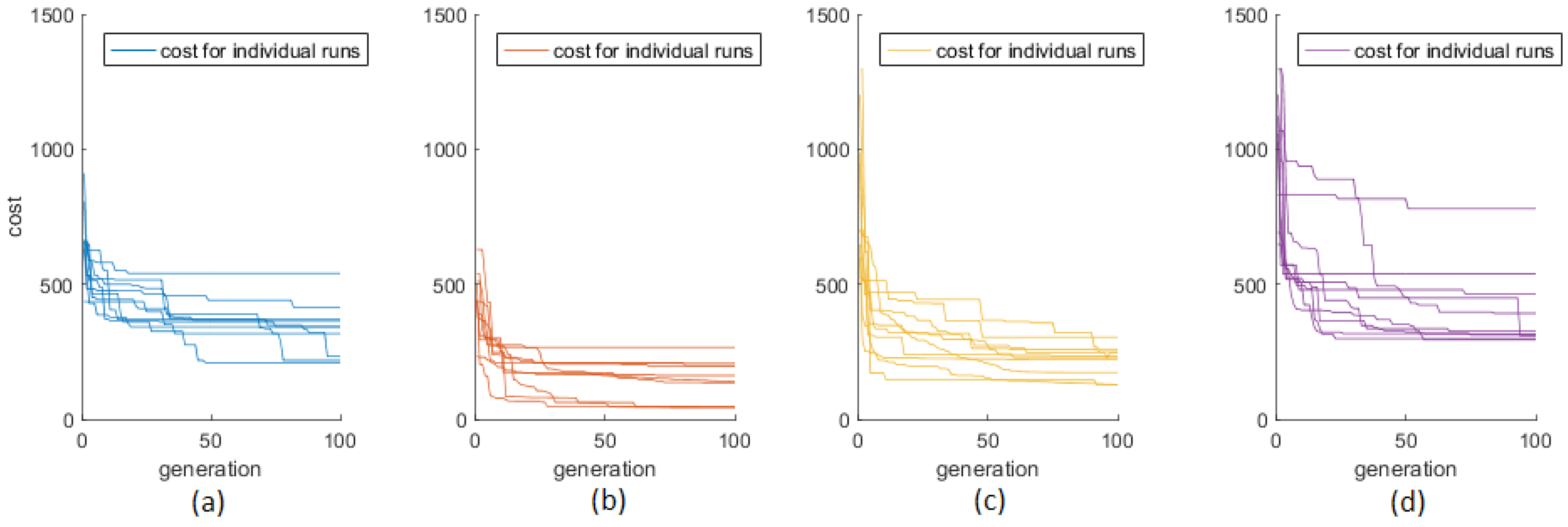
The stochastic nature of the genetic algorithms can be seen in Figure 11. The algorithm almost never finds the same configuration. It is, however, rather consistent in getting to the same fitness values. In this case, the manipulators with linear links perform with the lowest cost values.
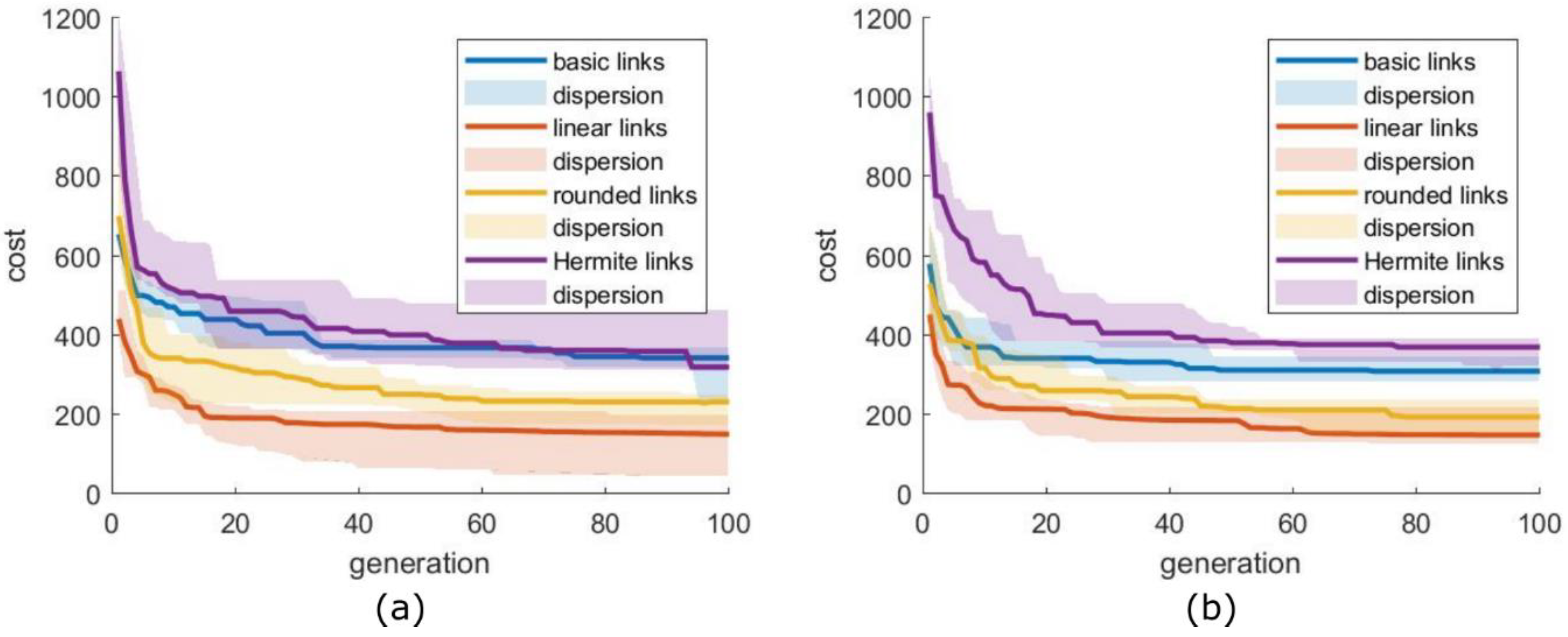
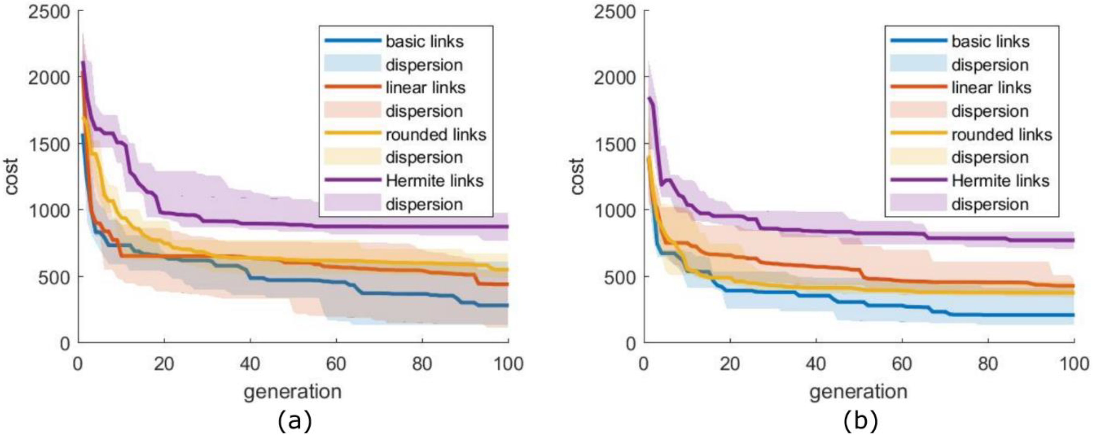
All 40 runs in Figure 11 are for task 1 and cost1. Putting the two together in one plot for comparison would result in an overcrowded graph; therefore, rather than showing them side-by-side as in Figure 11, we took the median values and presented them as single plots, as in Figure 12, Figure 13 and Figure 14. The dispersion is shown as an area between the 25th and 75th percentile.
With all tasks and cost functions, we saw better performance with simpler links (basic, linear, and rounded) and worse performance with the Hermite spline links. The differences between basic, linear and rounded links were task-dependent. Linear links performed well during task 1, however basic links were able to achieve lower cost values in the more geometrically complex task 3.
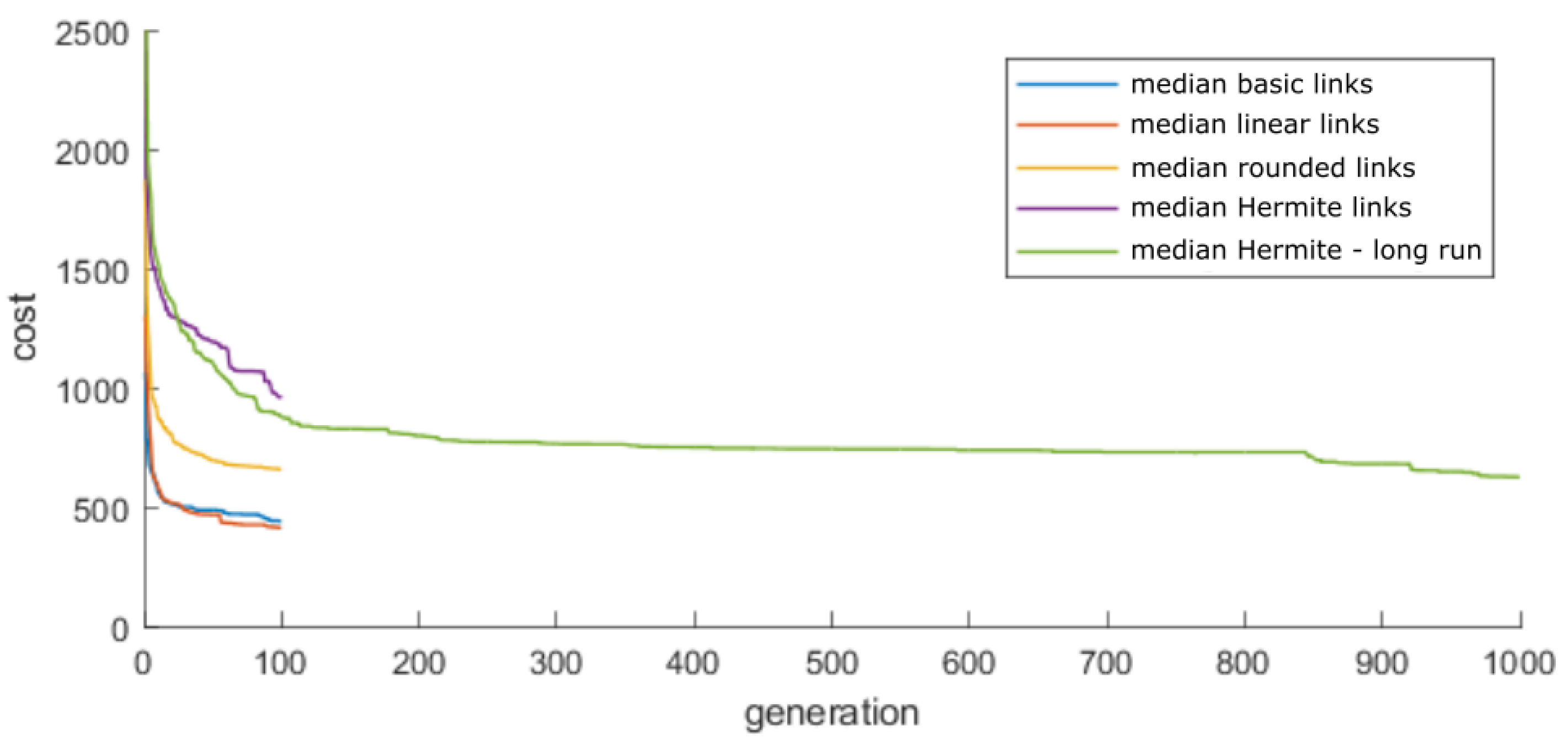
Slower convergence of Hermite spline links can be expected, since they are described with more parameters, which dramatically increases the search space. They are more adaptable, therefore they should be able to achieve better cost values across a longer run. To test this hypothesis, we selected task 2 and increased the number of generations from 100 to 1000. Figure 15 shows the results of this test.
As is visible from Figure 15, even a 10x increase in generations did not produce manipulators with cost values low enough to be comparable to our previous test. One run of the algorithm with 1000 generations takes about 22 h, which makes any practical use difficult.
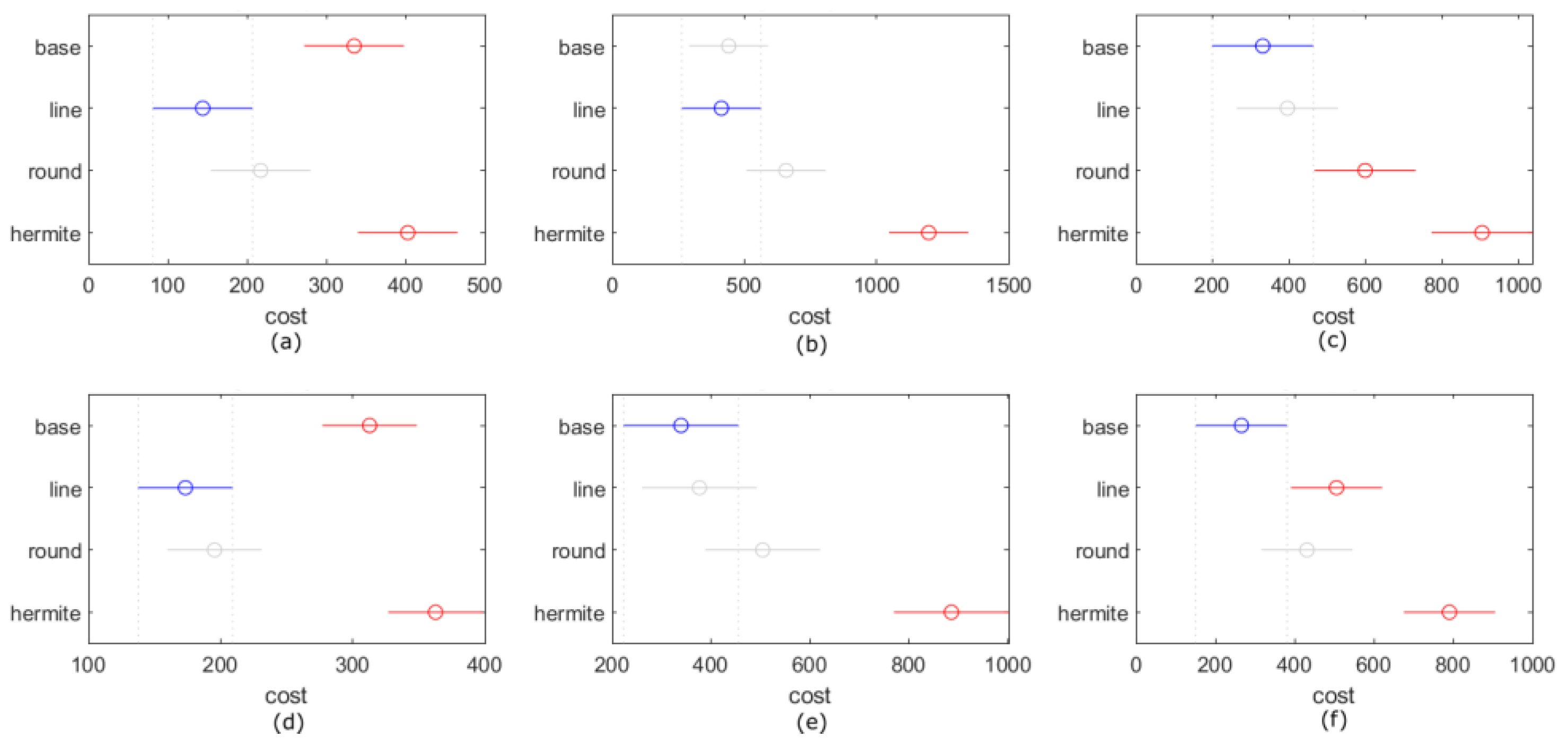
To inspect how significantly different each link type performs during the different tasks, we performed a one-way ANOVA analysis on the results of each GA run. Figure 16 shows mean estimates and comparison intervals at a significance level of 0.05. In the graphs, if the lines overlap vertically, the link types did not perform with significant difference.
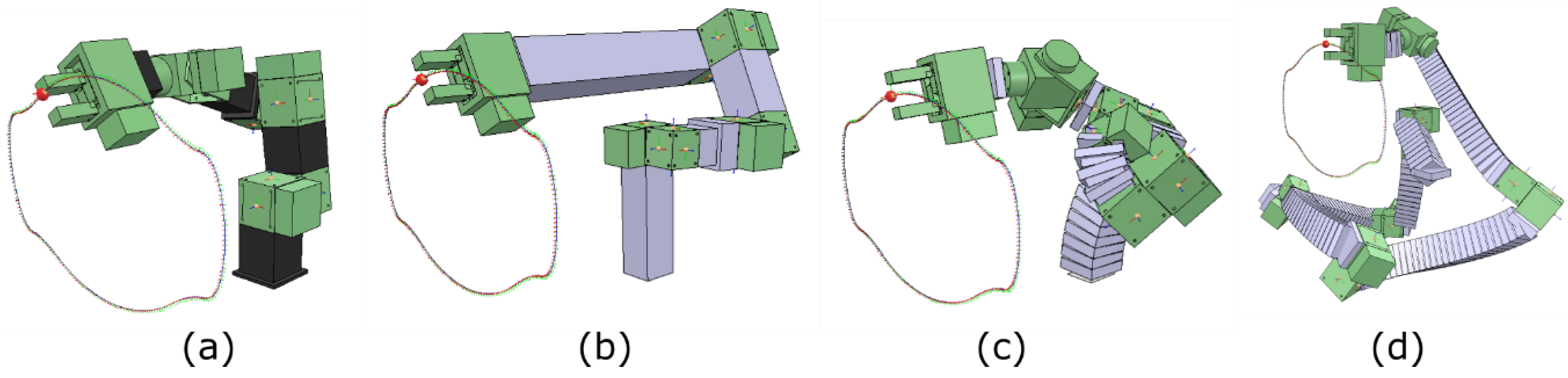
The best manipulators for each link type optimized with function cost2 are shown in Figure 17, Figure 18 and Figure 19.
It is apparent from the resulting structures that Hermite spline links occupy a larger volume, which might bring additional disadvantages. Additional tests with obstacles in the workspace might provide evidence that more adaptable links, such as Hermite spline links, can adapt to more complex environments. We considered optimizing manipulators with obstacles in the workplace to be outside of the scope of this article, however it is something we are planning to work on in the future.
4. Discussion
We implemented a method to test the performance of a genetic algorithm in terms of optimizing a manipulator with various mechanical links. Four different types of mechanical links located between the manipulator joints were implemented. The performance of the genetic algorithm was tested with various tasks and two cost functions.
We observed that optimizing a manipulator with a simple (basic, linear, or rounded) link type led to better results in all of our tests. The Hermite spline links underperformed even after a 10-fold increase in evaluations. It is possible that the increased search space caused by more parameters creates a combinatorial explosion and that increasing the generation count 10 times is not enough. There also could be certain fundamental disadvantages of spline-shaped links between joints. Further investigations with different types of splines could confirm this phenomenon.
When comparing the differences between the simpler types of joints, we observed that both rounded and linear links performed better than the basic links in task 1. However, in task 3, the linear links performed significantly better than linear or rounded links, depending on the used cost function. This could mean that the right choice of link type is task-specific or that basic links perform better on tasks with unchanging orientation of the end-effector. During task 2, the base, linear, and rounded links showed no statistically significant differences.
Including torque in the cost function did not have a significant effect on the results. This could be caused by the combined cost function, which was defined as a weighted sum of all of its parts. A multiobjective optimization method might be more effective in showing how much the torque measurements affect the results. This was considered outside the scope of this article, since we wanted to compare different types of links.
When examining the resulting kinematic structures for each task, we noticed that the solutions for task 1 with basic links resulted in more degrees of freedom. This could be caused by the distance between the trajectory and the robot base in combination with the length of the predefined links. Optimization produced manipulators with more DOF, and consequently a greater number of smaller links instead of longer links. The other types of links that were length-adjustable resulted in 3 or 4 DOF with longer links.
Overall, the simplicity of the genotype seems to be a significant factor when optimizing a manipulator for a specific task. Assembling the manipulator with curved links does not seem to provide any significant advantage, although we think that there still might be certain advantages in using curved links if a different optimization algorithm is used and there are obstacles in the environment.
5. Conclusions
In this work, we implemented a method to optimize and measure the performance of various mechanical links of an open-chain manipulator in task-specific conditions. Four different types of mechanical links connecting joints of the manipulator were implemented. These links included simple predefined links and links of variable length and curvature. The links were the basis for task-specific manipulators, which were optimized for three different tasks with varying levels of geometrical complexity.
Our initial assumption that the links with more configurable parameters would be able to better adapt to the task trajectory was disproven by the conducted tests. The simpler links were able to achieve significantly better performance in every task than the more complex Hermite spline links. The different simple links (either predefined basic links, linear links with adjustable length, or rounded links with adjustable length and curvature) generally showed similar performance, with notable differences depending on a given task.
Author Contributions
Conceptualization, Z.B.; methodology, Z.B. and R.P.; software, Z.B. and R.P.; validation, R.P., S.G., and D.H.; formal analysis, R.P.; investigation, S.G.; resources, D.H.; data curation, R.P.; writing—original draft preparation, R.P.; writing—review and editing, D.H. and S.G.; visualization, R.P.; supervision, Z.B.; project administration, Z.B.; funding acquisition, Z.B. All authors have read and agreed to the published version of the manuscript.
Funding
This work was supported by the European Regional Development Fund in the Research Center of Advanced Mechatronic Systems, project number CZ.02.1.01/0.0/0.0/16_019/0000867, within the Operational Program for Research, Development, and Education.
Institutional Review Board Statement
Not applicable.
Informed Consent Statement
Not applicable.
Data Availability Statement
The data presented in this study are available on request from the corresponding author. The data are not publicly available due to project restrictions.
Conflicts of Interest
The authors declare no conflict of interest.
References
- Brandstötter, M.; Angerer, A.; Hofbaur, M. The curved manipulator (Cuma-type arm): Realization of a serial manipulator with general structure in modular design. In Proceedings of the 2015 IFToMM World Congress, Taipei, Taiwan, 25–30 October 2015; pp. 403–409. [Google Scholar] [CrossRef]
- Nolfi, S.; Floreano, D. Evolutionary Robotics: The Biology, Intelligence, and Technology of Self-Organizing Machines, Book. 2000. Available online: https://books.google.cz/books?hl=cs&lr=&id=v300ui_1eZ4C&oi=fnd&pg=PP13&dq=evolutionary+robotics&ots=VPAzouWCOZ&sig=z3UPwz3PesFYzqATehtr-sa1hKI&redir_esc=y#v=onepage&q=evolutionaryrobotics&f=false (accessed on 21 October 2020).
- Back, T.; Hoffmeister, F. A survey of evolution strategies. In Proceedings of the Fourth International Conference on Genetic Algorithms, San Diego, CA, USA, 13–16 July 1991; Volume 2. Available online: http://www.academia.edu/download/47286951/A_Survey_of_Evolution_Strategies20160716-6237-p0d56x.pdf (accessed on 21 October 2020).
- Li, Z.; Lin, X.; Zhang, Q.; Liu, H. Evolution strategies for continuous optimization: A survey of the state-of-the-art. Swarm Evol. Comput. 2020, 56, 100694. [Google Scholar] [CrossRef]
- Chen, J.-C. Continual Learning for Addressing Optimization Problems with a Snake-Like Robot Controlled by a Self-Organizing Model. Appl. Sci. 2020, 10, 4848. [Google Scholar] [CrossRef]
- Respall, V.M.; Nolfi, S. Development of Multiple Behaviors in Evolving Robots. Robotics 2020, 10, 1. [Google Scholar] [CrossRef]
- Hauenstein, J.D.; Wampler, C.W.; Pfurner, M. Synthesis of three-revolute spatial chains for body guidance. Mech. Mach. Theory 2017, 110, 61–72. [Google Scholar] [CrossRef]
- Hornby, G.; Lipson, H.; Pollack, J. Generative representations for the automated design of modular physical robots. IEEE Trans. Robot. Autom. 2003, 19, 703–719. [Google Scholar] [CrossRef]
- Alattas, R.J.; Patel, S.; Sobh, T.M. Evolutionary Modular Robotics: Survey and Analysis. J. Intell. Robot. Syst. 2018, 95, 815–828. [Google Scholar] [CrossRef] [Green Version]
- Chung, W.K.; Han, J.; Youm, Y.; Kim, S.H. Task based design of modular robot manipulator using efficient genetic algorithm. In Proceedings of the IEEE International Conference on Robotics and Automation, Albuquerque, NM, USA, 20–25 April 1997; Volume 1, pp. 507–512. [Google Scholar] [CrossRef]
- Chocron, O.; Bidaud, P. Evolutionary algorithms in kinematic design of robotic systems. In Proceedings of the 1997 IEEE/RSJ International Conference on Intelligent Robot and Systems. Innovative Robotics for Real-World Applications. IROS ’97, Grenoble, France, 11 September 1997; Volume 2, pp. 1111–1117. [Google Scholar] [CrossRef]
- Valsamos, C.; Moulianitis, V.; Aspragathos, N. Index based optimal anatomy of a metamorphic manipulator for a given task. Robot. Comput. Manuf. 2012, 28, 517–529. [Google Scholar] [CrossRef]
- Valsamos, C.; Moulianitis, V.C.; Aspragathos, N. Metamorphic Structure Representation: Designing and Evaluating Anatomies of Metamorphic Manipulators. In Advances in Reconfigurable Mechanisms and Robots I; Springer: London, UK, 2012; pp. 3–11. [Google Scholar] [CrossRef]
- Katrantzis, E.F.; Aspragathos, N.A.; Valsamos, C.D.; Moulianitis, V.C. Anatomy Optimization and Experimental Verification of a Metamorphic Manipulator. In Proceedings of the 2018 International Conference on Reconfigurable Mechanisms and Robots (ReMAR), Delft, The Netherlands, 20–22 June 2018; pp. 1–7. [Google Scholar] [CrossRef]
- Patel, S.; Sobh, T. Task based synthesis of serial manipulators. J. Adv. Res. 2015, 6, 479–492. [Google Scholar] [CrossRef] [PubMed] [Green Version]
- Ha, S.; Coros, S.; Alspach, A.; Bern, J.M.; Kim, J.; Yamane, K. Computational Design of Robotic Devices from High-Level Motion Specifications. IEEE Trans. Robot. 2018, 34, 1–12. [Google Scholar] [CrossRef]
- Whitman, J.; Choset, H. Task-Specific Manipulator Design and Trajectory Synthesis. IEEE Robot. Autom. Lett. 2018, 4, 301–308. [Google Scholar] [CrossRef]
- Dogra, A.; Padhee, S.S.; Singla, E. An Optimal Architectural Design for Unconventional Modular Reconfigurable Manipulation System. J. Mech. Des. 2020, 1–29. [Google Scholar] [CrossRef]
- Liu, C.; Liu, J.; Moreno, R.; Veenstra, F.; Faíña, A. The impact of module morphologies on modular robots. In Proceedings of the 2017 18th International Conference on Advanced Robotics (ICAR), Hong Kong, China, 10–12 July 2017; pp. 237–243. [Google Scholar] [CrossRef] [Green Version]
- Moreno, R.; Faina, A. Using Evolution to Design Modular Robots: An Empirical Approach to Select Module Designs. In Lecture Notes in Computer Science (including Subseries Lecture Notes in Artificial Intelligence and Lecture Notes in Bioinformatics); Springer: Cham, Switzerland, 2020; Volume 12104, pp. 276–290. [Google Scholar] [CrossRef]
- Denavit, J.; Hartenberg, R.S. A kinematic notation for lower-pair mechanisms based on matrices. Trans. ASME E J. Appl. Mech. 1955, 22, 215–221. [Google Scholar]
- Ceccarelli, M.; Lanni, C. A multi-objective optimum design of general 3R manipulators for prescribed workspace limits. Mech. Mach. Theory 2004, 39, 119–132. [Google Scholar] [CrossRef]
- Singla, E.; Tripathi, S.; Rakesh, V.; Dasgupta, B. Dimensional synthesis of kinematically redundant serial manipulators for cluttered environments. Robot. Auton. Syst. 2010, 58, 585–595. [Google Scholar] [CrossRef]
- Rohmer, E.; Singh, S.P.N.; Freese, M. V-REP: A versatile and scalable robot simulation framework. In Proceedings of the IEEE International Conference on Intelligent Robots and Systems, Tokyo, Japan, 3–7 November 2013; pp. 1321–1326. [Google Scholar] [CrossRef]
- Lipow, P.R.; Schoenberg, I. Cardinal interpolation and spline functions. III. Cardinal Hermite interpolation. Linear Algebra Appl. 1973, 6, 273–304. [Google Scholar] [CrossRef] [Green Version]
- Mitchell, M. An Introduction to Genetic Algorithms; MIT Press: Cambridge, MA, USA, 2020. [Google Scholar]
- Brandstötter, M. Adaptable Serial Manipulators in Modular Design. Ph.D. Dissertation, UMIT, Institute of Automation and Control Engineering, Hall in Tirol, Austria, November 2016. [Google Scholar] [CrossRef]
Figure 1.
Example of a manipulator with links, joints, and an end-effector.

Figure 2.
Schunk joint modules: (a) PR 70; (b) PR 90; (c) PW 70. The simulated counterparts: (d) PR 70; (e) PR 90; (f) PW 70.
Figure 2.
Schunk joint modules: (a) PR 70; (b) PR 90; (c) PW 70. The simulated counterparts: (d) PR 70; (e) PR 90; (f) PW 70.

Figure 3.
Types of links: (a) basic; (b) linear; (c) rounded; (d) Hermite spline.

Figure 4.
ID numbers for the basic manipulator links.

Figure 5.
An example of a chromosome with a highlighted crossover point.

Figure 6.
Rounded link gene mutation: (a) before; (b) after.

Figure 7.
Flowchart of the collision calculation.

Figure 8.
Task 1: (a) position; (b) orientation.

Figure 9.
Task 2: (a) position; (b) orientation.

Figure 10.
Task 3: (a) position; (b) orientation.

Figure 11.
All runs for trajectory task 1 and cost function cost1: with (a) basic links; (b) linear links; (c) rounded links; (d) Hermite spline links.
Figure 11.
All runs for trajectory task 1 and cost function cost1: with (a) basic links; (b) linear links; (c) rounded links; (d) Hermite spline links.

Figure 12.
Results for task 1: (a) cost1; (b) cost2.

Figure 13.
Results for task 2: (a) cost1; (b) cost2.

Figure 14.
Results for task 3: (a) cost1; (b) cost2.

Figure 15.
Results for a longer run of Hermite spline links for task 2 and function cost1.

Figure 16.
ANOVA results. The links with lowest cost value are shown in blue, links that are not significantly different from the best one are shown in gray, and links that are significantly different are shown in red: (a) task 1, cost1; (b) task 2, cost1; (c) task 3, cost1; (d) task 1, cost2; (e) task 2, cost2; (f) task 3, cost2.

Figure 17.
Best results for task 1: (a) basic links; (b) linear links; (c) rounded links; (d) Hermite spline links.
Figure 17.
Best results for task 1: (a) basic links; (b) linear links; (c) rounded links; (d) Hermite spline links.

Figure 18.
Best results for task 2: (a) basic links; (b) linear links; (c) rounded links; (d) Hermite spline links.
Figure 18.
Best results for task 2: (a) basic links; (b) linear links; (c) rounded links; (d) Hermite spline links.

Figure 19.
Best results for task 3: (a) basic links; (b) linear links; (c) rounded links; (d) Hermite spline links.
Figure 19.
Best results for task 3: (a) basic links; (b) linear links; (c) rounded links; (d) Hermite spline links.


Table 1.
Joint module physical parameters.
| Parameter | PR 70 | PR 90 | PW 70 (axis1, axis2) |
|---|---|---|---|
| Maximal torque | 46 Nm | 145 Nm | 24 Nm, 4 Nm |
| Weight | 1.7 kg | 3.6 kg | 1.8 kg |
| Maximal current | 8 A | 12 A | 8 A, 6.5 A |
| Flange size | 70 mm | 90 mm | 70 mm |
| Type ID (in the program) | 0 | 1 | 2 |
Table 2.
Joint module parameters used for optimization.
| Parameter | Range (Limits for Optimization) |
|---|---|
| ID | {0, 1, 2} |
| ora | {0, π/2, π, 3π/2} |
| orb | {0, π/2, π, 3π/2} |
Table 3.
Link parameters.
| Modular Link Type | Parameter/Parameters | Range (Limits for Optimization) |
|---|---|---|
| Basic | ID | {0, 12} |
| Linear | Length (L) | {35, 500} [mm] |
| Rounded | Circumferential length (L) | {35, 500} [mm] |
| Turn radius (R) | {10, 500} [mm] | |
| Turn direction angle (α) | {0, 180} [deg] | |
| Hermite spline | Normal 1 (n1) | {1, 300} [mm] |
| End X (px) | {−500, 500} [mm] | |
| End Y (py) | {−500, 500} [mm] | |
| End Z (pz) | {−500, 500} [mm] | |
| Bend (γ) | {−90, 90} [deg] | |
| Twist (β) | {−90, 90} [deg] | |
| Normal 2 (n2) | {1, 300} [mm] |
Table 4.
Parameters of the basic links.
| Link ID | 1 | 2 | 3 | 4 | 5 | 6 | 7 | 8 | 9 | 10 | 11 | 12 |
|---|---|---|---|---|---|---|---|---|---|---|---|---|
| Flange size [mm] | 70 | 70 | 70 | 70 | 70 | 90,70 | 90,70 | 90,70 | 90 | 90 | 90 | 90 |
| Length [mm] | 35 | 70 | 140 | 210 | 70 | 45 | 90 | 180 | 45 | 90 | 180 | 270 |
Publisher’s Note: MDPI stays neutral with regard to jurisdictional claims in published maps and institutional affiliations. |
© 2021 by the authors. Licensee MDPI, Basel, Switzerland. This article is an open access article distributed under the terms and conditions of the Creative Commons Attribution (CC BY) license (http://creativecommons.org/licenses/by/4.0/).
Share and Cite
MDPI and ACS Style
Pastor, R.; Bobovský, Z.; Huczala, D.; Grushko, S. Genetic Optimization of a Manipulator: Comparison between Straight, Rounded, and Curved Mechanism Links. Appl. Sci. 2021, 11, 2471. https://doi.org/10.3390/app11062471
AMA Style
Pastor R, Bobovský Z, Huczala D, Grushko S. Genetic Optimization of a Manipulator: Comparison between Straight, Rounded, and Curved Mechanism Links. Applied Sciences. 2021; 11(6):2471. https://doi.org/10.3390/app11062471
Chicago/Turabian StylePastor, Robert, Zdenko Bobovský, Daniel Huczala, and Stefan Grushko. 2021. "Genetic Optimization of a Manipulator: Comparison between Straight, Rounded, and Curved Mechanism Links" Applied Sciences 11, no. 6: 2471. https://doi.org/10.3390/app11062471
Note that from the first issue of 2016, this journal uses article numbers instead of page numbers. See further details here.