Smoothed Particle Hydrodynamics Simulation of Orthogonal Cutting with Enhanced Thermal Modeling

Abstract

Smoothed Particle Hydrodynamics (SPH) is a mesh-free numerical method that can simulate metal cutting problems efficiently. The thermal modeling of such processes with SPH, nevertheless, is not straightforward. The difficulty is rooted in the computationally demanding procedures regarding convergence properties and boundary treatments, both known as SPH Grand Challenges. This paper, therefore, intends to rectify these issues in SPH cutting models by proposing two improvements: (1) Implementing a higher-order Laplacian formulation to solve the heat equation more accurately. (2) Introducing a more realistic thermal boundary condition using a robust surface detection algorithm. We employ the proposed framework to simulate an orthogonal cutting process and validate the numerical results against the available experimental measurements.

1. Introduction

Metal cutting is one of the essential processes throughout engineering designs and manufacturing industries. In order to reduce costs and increase productivity, it is necessary to improve understanding of the metal cutting problem. As there is a wide range of design variables (e.g., tool wear, workpiece temperature, process forces, chip shape, or surface quality) and diverse physical phenomena; nonetheless, the reliability of empirical and analytical models for metal cutting is limited. In this view, computer-based simulations using numerical methods appear as an invaluable alternative to study metal cutting problems with deeper insights.

In addition to the well-known Finite Element Method (FEM), the family of particle-based methods is another numerical approach frequently used for cutting simulations. Unlike FEM, however, these methods do not require re-meshing as they are mesh-free. This interesting feature of particle methods makes them a suitable choice for metal cutting applications. In particular, the Smoothed Particle Hydrodynamics (SPH) method, introduced independently by Gingold et al. [1] and Lucy [2] in 1977, sees a broader spectrum of applications in this context. SPH is known as a well-established numerical tool for modeling fluid dynamics. Examples include the application in impact [3] and shockwave [4] simulations, complex free-surface problems [5], and thermal simulation of multiphase flows by [6,7]. The utilization of SPH in more industrially-oriented fields of application can also be found in the literature. Examples in laser-based manufacturing problems are the modeling of material removal in [8,9] and pulsed-laser ablation of aluminum in [10].

Between 2007 and 2015, numerous researchers applied SPH to metal cutting and the chip formation, including the high-speed cutting [11,12] and 3D single-grain [13] models using commercial software packages, as well as the developments in [14,15] using an in-house code. These papers do not consider the heat transfer from the workpiece to the tool, while the experimental evidence has shown that a significant proportion of heat in metal machining operations transfers from the chipping zone to the cutting tool [16]. More recently, the concept of parallel computing on Graphics Processing Units (GPU) has been introduced to both 2D [17] and 3D [18] SPH cutting simulations to boost the computational performance. Afrasiabi et al. [19] employed this GPU-accelerated approach for inverse parameter identification and proposed a temperature-dependent coefficient of friction in SPH cutting models. Furthermore, a tailor-made framework for the multi-resolution SPH simulation of orthogonal cutting tests was published by [20]. It is worth mentioning that the computer codes utilized by these recent works are open source.

Although previous studies have demonstrated some excellent results in the capability of SPH to simulate metal cutting processes, none of them accounts for heat loss boundary conditions in their thermal model. More specifically, the issue with ignoring the heat transfer from the workpiece to the tool in SPH models (e.g., in [13,20]) was addressed by some recent works in [17,19]. However, the thermal modeling approach in these papers also suffers from two shortcomings: (1) Utilizing an inconsistent Laplacian operator that deteriorates the solution accuracy near the boundaries. (2) Neglecting the convective and radiative heat loss from the system. Consequently, we intend to develop a comprehensive thermal model for SPH cutting simulations that resolve these issues and account for all these effects.

In this work, a numerical simulation framework is developed that can increase the reliability of available mesh-free cutting models in their thermal modeling approach. As the first task, boundary particles are identified by a robust surface detection algorithm [5] borrowed from the CFD community. The present thermal model contains (1) heat generation due to the plastic and frictional work, (2) heat transfer from the workpiece to the tool, (3) heat conduction in the whole system, and (4) both Dirichlet and von Neumann boundary conditions. To address the inconsistency issue of SPH formulations, an adaptation of Fatehi’s scheme [21] (FMFS) is additionally used, which introduces an approximation of the Laplace operator of second-order consistency. This method is implemented here for the first time in solid mechanics problems with large deformations. For an application of FMFS in 3D heat conduction problems with no deformations, see in [22]. Please note that the results presented here are produced by the open-source codes for SPH metal cutting, which are available online and given in the “Supplementary Materials” section of this article.

2. Governing Equations

Before presenting the numerical framework for modeling of a cutting process, we provide an overview of the underlying physics in this section. The drawings in Figure 1 show a graphical illustration of the key thermal aspects of metal cutting. In these figures, the main heat sources associated with each deformation zone are shown, as well as a representation of the thermal boundary conditions.

The continuum mechanical equations in a Lagrangian formalism are expressed by the field equations:

$$\begin{array}{cc}\hfill \frac{d\rho }{dt}& =-\rho \nabla ·\underset{¯}{v}\hfill \end{array}$$

(1)

$$\begin{array}{cc}\hfill \frac{d\underset{¯}{v}}{dt}& =\frac{1}{\rho }\nabla ·\underset{=}{\sigma }+\frac{1}{\rho }\underset{¯}{b}\hfill \end{array}$$

(2)

$$\begin{array}{cc}\hfill \frac{d\underset{¯}{r}}{dt}& =\underset{¯}{v}\hfill \end{array}$$

(3)

where $\rho$ is the density, $\underset{¯}{r}$ the position vector, $\underset{¯}{v}$ the velocity, $\underset{=}{\sigma }$ the Cauchy stress tensor, and $\underset{¯}{b}$ the volumetric body forces. It is worth mentioning that all numerical simulations in this work are based on single-resolution SPH formulations; thus, a uniform constant mass is allocated to each computational node and the momentum equation (i.e., Equation (2)) does not require the utilization of mass scaling. An elaboration of this subject, as well as further details on the numerical stabilization procedure, can be found in [19,20]. This mechanical system is coupled with thermal effects by solving the heat conduction equation:

$$\begin{array}{c}\hfill \frac{dT}{dt}=\frac{k}{\rho c_p}{\nabla }^{2}T+\frac{1}{\rho c_p}(Q^{\mathrm{plast}}+Q^{\mathrm{fric}})\end{array}$$

(4)

in which k is the heat conductivity assuming an isotropic heat conduction, $c_p$ the specific isobaric heat capacity, including the source terms $Q^{\mathrm{plast}}$ and $Q^{\mathrm{fric}}$ due to the conversion of the plastic and frictional work. According to the works in [17,23], these heat sources are computed from

$$\begin{array}{cc}\hfill Q^{\mathrm{plast}}& =\chi \left({\sigma }_y{\dot{\overline{\epsilon }}}^{pl}\right)\hfill \end{array}$$

(5)

$$\begin{array}{cc}\hfill Q^{\mathrm{fric}}& =\eta \left(\frac{\rho |{\underset{¯}{f}}^{\mathrm{fric}}|·|{\underset{¯}{v}}^{\mathrm{rel}}|}{m}\right)\hfill \end{array}$$

(6)

if $\chi$ and $\eta$ are dimensionless parameters specifying the fraction of plastic and frictional work converted into heat (see in [23,24]). According to the illustration in Figure 1, the boundary conditions of Equation (4) are given by

$$\begin{array}{cccc}\hfill T_c& =T_{\infty }\hfill & \hfill ⟶& \mathrm{on}\mathrm{fixed}\mathrm{boundaries}\hfill \end{array}$$

(7)

$$\begin{array}{cccc}\hfill q_l& =-[\underset{\mathrm{convection}}{\underbrace{h_c(T_s-T_{\infty })}}+\underset{\mathrm{radiation}}{\underbrace{ϵ\sigma (T_s^4-T_{\infty }^4)}}]\hfill & \hfill ⟶& \mathrm{on}\mathrm{open}\mathrm{boundaries}\hfill \end{array}$$

(8)

with $h_c$ denoting the heat convection coefficient, $T_s$ and $T_{\infty }$ the surface and background temperatures, respectively; $ϵ$ the emissivity factor; and $\sigma$ the Stefan–Boltzmann constant.

For material modeling, the Johnson–Cook (JC) flow stress according to [25] is used to define the plastic response of the workpiece material. This model calculates the flow stress of the material, ${\sigma }_y$, and incorporates three effects: strain hardening, strain rate hardening, and thermal softening. The JC flow stress is computed from

$${\sigma }_y^{\mathrm{JC}}=[A+B{\left({\overline{\epsilon }}^{pl}\right)}^n][1+Cln\left(\frac{{\dot{\overline{\epsilon }}}^{pl}}{{\dot{\overline{\epsilon }}}_0^{pl}}\right)][1-{\left(\frac{T-T_r}{T_m-T_r}\right)}^m]$$

(9)

where ${\overline{\epsilon }}^{pl}$ is the equivalent plastic strain and $T_r$ and $T_m$ are the reference temperature and melting point, respectively. In Section 5, the values of five JC parameters ($A,B,C,m$, and n) will be provided for the titanium alloy under consideration.

For friction modeling, Coulomb’s law with a constant coefficient of $\mu =0.35$ is considered as a typical choice in LS-DYNA [13] and other SPH cutting models like [17], unless otherwise mentioned. As the magnitude of $\mu$ has a significant impact on the force prediction of numerical cutting models (see in [19,26] for more details), a sensitivity analysis will be presented to provide further insights into the influence of the friction coefficient on simulation results.

3. SPH Formulation

The partial differential equations (PDEs) outlined in Equations (1), (2), and (4) need to be discretized in space and time. The spatial discretization is performed by applying an stabilized SPH scheme. Liu et al. [27] provide a good overview of the SPH formulations and its derivation details. The time discretization is then carried out using an explicit second-order leapfrog stepping. Monaghan [28] provides the implementation procedure of this time integration scheme for SPH models.

Using a modified SPH approach expressed in [29,30], the mass, momentum, and heat equations for particle i can be written in the following discrete forms:

$$\begin{array}{cc}\hfill {〈\frac{d\rho }{dt}〉}_i& \approx -{\rho }_i\sum _j({\underset{¯}{v}}_j-{\underset{¯}{v}}_i)·\nabla W_{ij}{V}_j\hfill \end{array}$$

(10)

$$\begin{array}{cc}\hfill {〈\frac{d\underset{¯}{v}}{dt}〉}_i& \approx \sum _j\left(\frac{{\underset{=}{\sigma }}_i}{{\rho }_i^2}+\frac{{\underset{=}{\sigma }}_j}{{\rho }_j^2}+\underset{\mathrm{stabilizers}}{\underbrace{{\mathsf{\Pi }}_{ij}\underset{=}{I}+{\underset{=}{\mathsf{\Lambda }}}_{ij}}}\right)·\nabla W_{ij}{m}_j+\frac{1}{m_i}{\underset{¯}{b}}_i\hfill \end{array}$$

(11)

$$\begin{array}{cc}\hfill {〈\frac{dT}{dt}〉}_i& \approx \frac{k}{\rho c_p}\sum _{j}2\left[\left(\frac{T_i-T_j}{|r_{ij}|}\right){\underset{¯}{e}}_{ij}·\nabla W_{ij}\right]V_j+{\left(\frac{Q^{\mathrm{plast}}+Q^{\mathrm{fric}}}{\rho c_p}\right)}_i\hfill \end{array}$$

(12)

where $V_j=m_j/{\rho }_j$ is the integration volume of particle j and $W_{ij}=W_h({\underset{¯}{r}}_i-{\underset{¯}{r}}_j,h)$ is a kernel function with the smoothing length h, chosen to be the cubic B-spline function [31] in this work. Furthermore, $\mathsf{\Pi }$ and $\underset{=}{\mathsf{\Lambda }}$ are the artificial viscosity term [32] and the artificial stress tensor [33] with the parameters taken similarly as in [17,19]. For the heat equation expressed in Equation (12), the method suggested by Brookshaw [30] is considered to discretize the Laplacian operator, where ${\underset{¯}{e}}_{ij}={\underset{¯}{r}}_{ij}/\left|r_{ij}\right|$ is a unit vector in the inter-particle direction. After computing these equations for each particle, the particles position $\underset{¯}{r}$ is updated with a smoothed velocity instead of the actual velocity. This smoothing scheme was introduced by Monaghan [34] and is called the X-SPH correction. The same X-SPH parameter as [17,19] is used for the numerical simulations of this work.

4. Proposed Thermal Model

The key contribution of this work to the SPH cutting models is the enhancement it proposes for thermal modeling. First, a higher-order Laplacian approximation is presented to replace the Brookshaw scheme in the heat equation. Next, the proposed approach for handling thermal boundary conditions is described.

4.1. Discretization of Laplacian

The Laplacian approximation model considered in this paper was initially proposed by Fatehi et al. [21]. They came up with a novel renormalization matrix $\underset{¯}{\underset{¯}{G}}$ that mitigates the boundary deficiency issue in SPH formulations by re-normalizing the kernel function. Fatehi’s mesh-free scheme is here referred to as FMFS for brevity. In short, the FMFS operator for the discretization of ${\nabla }^{2}T$ at particle i reads

$$\begin{array}{cc}\hfill {〈{\nabla }^{2}T〉}_i& \approx {\underset{¯}{\underset{¯}{G}}}_i:\sum _{j}2\left(\left(\frac{T_j-T_i}{|{\underset{¯}{r}}_{ij}|}-{\underset{¯}{e}}_{ij}·\sum _j(T_j-T_i){\underset{¯}{\underset{¯}{A}}}_i·\nabla W_{ij}{V}_j\right){\underset{¯}{e}}_{ij}\otimes \nabla W_{ij}\right)V_j\hfill \end{array}$$

(13)

$$\begin{array}{cc}\hfill {\underset{¯}{\underset{¯}{A}}}_i& ={\left[\sum _j\left({\underset{¯}{r}}_{ji}\otimes \nabla W_{ij}\right)V_j\right]}^{-1}\hfill \end{array}$$

(14)

where “:” denotes the double contraction of two second-order tensors, “⊗” indicates the tensor product, and the definition of $\underset{¯}{\underset{¯}{G}}$ correction tensor is given in [21,22,35]:

$${\underset{¯}{\underset{¯}{G}}}_i:\left[\sum _j\left({\underset{¯}{e}}_{ij}\otimes {\underset{¯}{e}}_{ij}\otimes \nabla W_{ij}\right)V_j·{\underset{¯}{\underset{¯}{A}}}_i^{-1}·\sum _j\left({\underset{¯}{r}}_{ij}\otimes {\underset{¯}{r}}_{ij}\otimes \nabla W_{ij}\right)V_j+\sum _j\left({\underset{¯}{r}}_{ij}\otimes {\underset{¯}{e}}_{ij}\otimes {\underset{¯}{e}}_{ij}\otimes \nabla W_{ij}\right)V_j\right]=-\underset{=}{I}$$

(15)

Derivation details of this method, as well as its application to several 3D benchmark tests, can be found in [22]. According to the reconstruction examples presented in [21,22], the approximation procedure of Equation (13) reproduces Laplacian results that are second-order consistent and converge quadratically.

4.2. Thermal Boundary Conditions

The boundary conditions expressed in Equations (7) and (8) need to be imposed on surface particles at each time step. The identification of particles located at the clamped surfaces is trivial and can be done once at the initial configuration. However, the detection of particles belonging to the open surfaces of the workpiece cannot be done without utilizing a particular measure. To do so, we incorporate a free-surface detection algorithm initially formulated by Marrone et al. [5] in fluid flow problems.

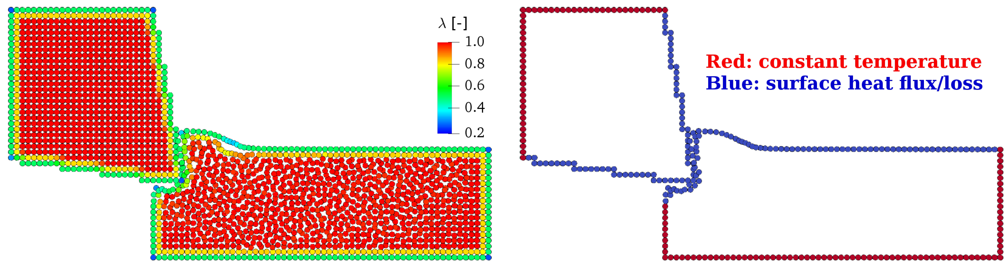
In this algorithm, the parameter $\lambda$ is calculated as the minimum eigenvalue of the matrix $\underset{¯}{\underset{¯}{A}}$ in Equation (14), also known as the Randles–Liberky [36] renormalization matrix. Theoretically, the values of $\lambda$ vary from 0 to 1 for exterior and interior particles, respectively. Preliminary studies by the authors of [5] demonstrated that taking a $\lambda =0.75$ is generally a proper choice as it isolates at least one layer of surface particles. Figure 2 confirms this by displaying one example frame of an orthogonal cutting simulation with SPH, where the surface detection algorithm is active in the code. It demonstrates how the surface particles required for thermal boundary conditions can be effectively identified using this algorithm. Another advantage of detecting surface particles is linked with the stability of the Laplacian formulation. That is, Fatehi’s Laplacian operator Equation (13) is computed for interior particles ($\lambda ⩾0.75$), and the approximation of the heat equation for all surface particles falls back to Brookshaw’s method in Equation (4). By doing so, the singularity of correction matrices in FMFS can be avoided. This matter has been elaborated by Afrasiabi et al. [22] in several 3D heat conduction benchmark tests.

5. Results & Discussion

Before applying the higher-order SPH method (i.e., FMFS) to a metal cutting problem, we showcase a simple mathematical function to validate the implementation of Equation (13) and examine its improvement versus the Brookshaw SPH expressed in Equation (12).

5.1. Preliminary Study

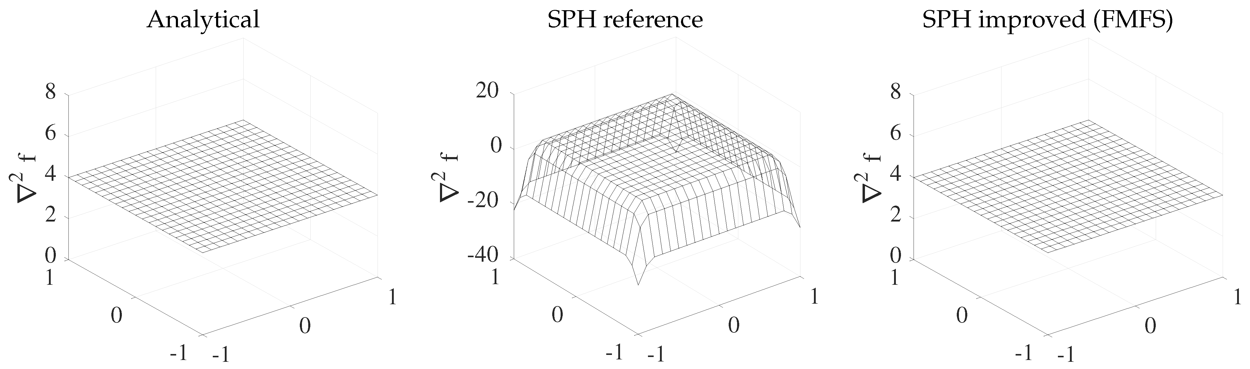
In this example, the Laplacian of $f(x,y)=x^2+y^2$ is computed in a domain of $(x,y)\in [-1+1]$ discretized by $21\times 21$ uniformly spaced particles, for which the analytical answer is given by ${\nabla }^{2}f(x,y)=+4$. This choice was made to verify the second-order consistency of the FMFS approximation. As mentioned before, the cubic B-spline kernel with a smoothing length of $h=1.5\Delta x$ is used.

Figure 3 demonstrates the surface plots of numerical solutions, where FMFS recovers second-order consistency by producing exact results throughout the domain. In the case of using the reference SPH method, as shown in the middle plot of Figure 3, severe inconsistencies resulting from the boundary deficiency of SPH exist outside the range of $[-0.8+0.8]$. The computations show that the Laplacian result using the reference SPH model is approximately +4.027 within $[-0.8+0.8]$. Outside this range, the approximation error of $\langle {\nabla }^{2}f\rangle$ increases drastically and reaches its maximum value at four corners. The approximate value of Laplacian at these points is −22.12, corresponding to a relative error of 453%. As discussed already, the FMFS method employed by the proposed thermal model resolves this issue by incorporating higher-order terms and kernel renormalization, giving exact results with no error.

This preliminary investigation indicates that boundary effects can deteriorate the accuracy of the SPH Laplacian operator. Indeed, this situation occurs in metal cutting problems, where the thermal boundary conditions are associated with high surface temperatures, especially in the chip formation zone. By applying FMFS in the proposed thermal model, the heat equation in SPH metal cutting simulations is solved more accurately at the price of a higher computational cost.

5.2. Application: Orthogonal Metal Cutting

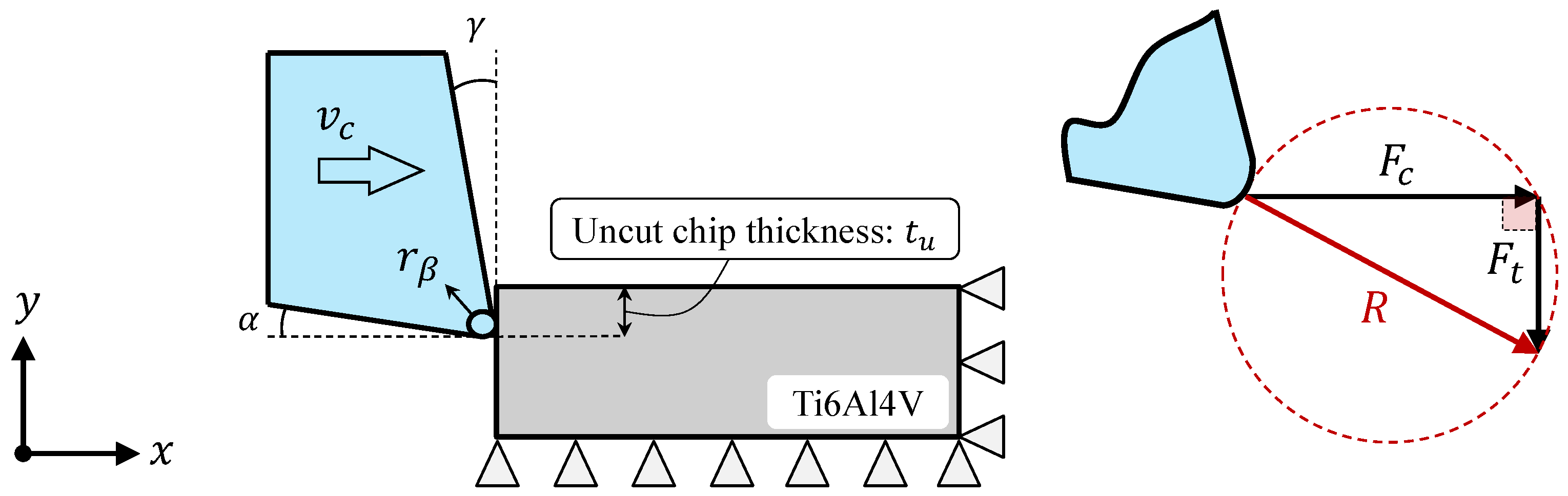
After validating the implementation of the higher-order Laplacian model, a 2D simulation of the orthogonal cutting of a Ti6Al4V titanium alloy is carried out using the process parameters and problem dimension listed in

Table 1. Experimental and numerical parameters for the cutting test, according to the works in [17,19]. Thermo-physical properties required for thermal convection and radiation are taken from the works in [38].

Body	Property	Symbol	Unit	Value
Tool	Clearance angle	$\alpha$	deg	7
	Rake angle	$\gamma$	deg	0
	Cutting edge radius	$r_{\beta }$	mm	0.0028
	Speed	$v_c$	m min${}^{-1}$	318.5
	Heat conductivity	k	W m${}^{-1}$ K${}^{-1}$	88
	Specific heat capacity	$c_p$	J kg${}^{-1}$ K${}^{-1}$	292
Workpiece	Length	$l_x$	mm	3
	Height	$l_y$	mm	0.3
	Uncut chip thickness	$t_u$	mm	0.1
	Cut distance	$l_c$	mm	2
	Density	$\rho$	kg m${}^{-3}$	4430
	Young’s modulus	E	GPa	113.8
	Poisson ratio	$\nu$	–	0.35
	Heat conductivity	k	W m${}^{-1}$ K${}^{-1}$	7.3
	Specific heat capacity	$c_p$	J kg${}^{-1}$ K${}^{-1}$	580
	Reference temperature	$T_r$	K	300
	Melting temperature	$T_m$	K	1878
	Coeff. of friction	$\mu$	–	0.35
	Pct. of plastic work into heat	$\chi$	–	90%
	Pct. of frictional work into heat	$\eta$	–	100%
All	Convection coeff.	$h_c$	W m${}^{-2}$ K${}^{-1}$	50.0
	Emissivity coeff.	$ϵ$	–	0.30
	Stefan–Boltzmann constant	$\sigma$	W m${}^{-2}$ K${}^{-4}$	$5.67\times {10}^{-8}$

. For this material, the JC parameters $A=862$ MPa, $B=331$ MPa, $C=0.01$, $m=0.8$, and $n=0.35$ are chosen, according to the works in [17,19,25] for very similar applications. Figure 4 shows the geometry and boundary conditions for this problem, where a Dirichlet temperature boundary condition of $T_c=T_{\infty }=300$ K is imposed on the fixed layers (see Figure 2). The SPH simulation runs until 2/3 of the workpiece length is cut with a speed of $v_c=318.5$ m/min. This choice of the cut distance is made to ensure that the solution is not affected by the fixed boundary condition (see the right side of the Ti6Al4V workpiece in Figure 4). Moreover, it leads to a cut distance of 2 mm, which is much longer than what is needed to reach the steady-state forces at this high cutting speed [37].

A total of 41 particles (with regular spacing) along $l_y$ are used to discretize the workpiece. Clearly, using SPH particles of different sizes leads to computationally more efficient discretizations. Due to the ease of computer implementation and for more simplicity, however, the present work considers a uniform spacing of SPH particles in all simulations. For implementing the thermal model throughout the system, it is necessary to discretize the cutting tool as well. In this paper, the size of SPH particles in the tool is set to be equal to the size of SPH particles in the workpiece. It is important to note that the heat equation on the tool side can also be solved by the finite-difference or finite-element methods. While these mesh-based approaches are generally more efficient than SPH in thermal modeling, they are not implemented here as the utilization of a hybrid particle-element technique is beyond the scope of this paper.

5.2.1. Force Prediction and Chip Shape

Among the provided experimental dataset, the highest cutting speed of $v_c=318.5$ m/min was chosen for the SPH models of this paper to attain the shortest simulation time. The elapsed time per 2 mm cut distance is in the range of 29 h for this cutting speed, with a single core of Intel^® i5-4690 at 3.50 GHz. Furthermore, the orthogonal cutting experiment was conducted by setting a rake angle of $\gamma =0$° in order to obtain a state, where the thrust force ($F_t$ in Figure 4) is mainly caused by the friction between the rake face and the sliding chip.

For the experimentation, we conducted turning operations as orthogonal cutting tests on a Ti6Al4V cylinder with a diameter of about 70 mm and a wall thickness of 2 mm. The insert in its holder was held on the tool turret of the CNC turning machine. Both cutting and feed forces ($F_c$ and $F_t$) were measured with a 3D Kistler piezoelectric force sensor.

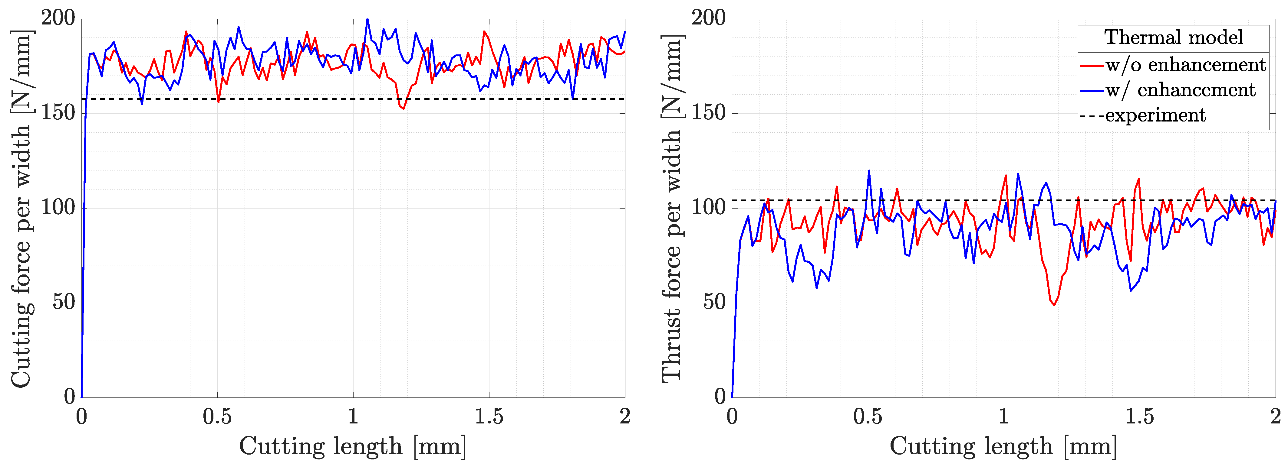
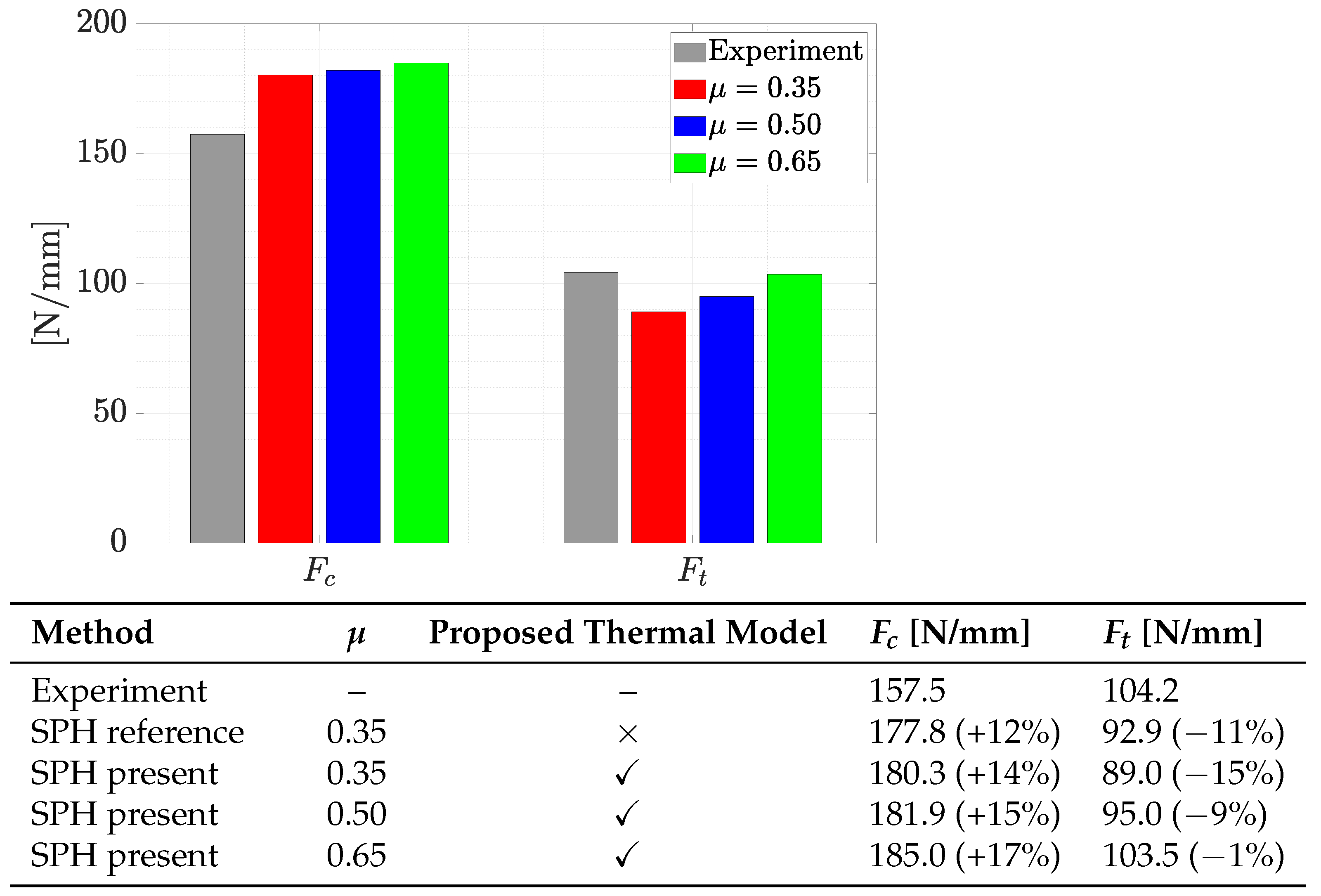
The numerical simulation is first validated by comparing the predicted forces with the experimental measurements. Figure 5 plots the evolution of these forces during 2 mm of this cutting process. An average of the predicted forces is calculated at the stationary zone, after almost 10% of the simulation time is elapsed. These average forces are listed in Figure 6, showing that both $F_c$ and $F_t$ computed from the simulation compare very well with the experimental data. The percent errors given in parentheses in this table shows an average of approximately 14% overprediction for $F_c$ and 9% underprediction for $F_t$.

According to the thrust force plot in Figure 5, the overall maximum discrepancy between the experimental and numerical results produces an error of 53% underprediction for SPH with the reference model (see the red line at about 1.2 mm cutting length). When using the proposed model, this value is reduced to 45% and occurs slightly before 1.5 mm of the cutting length. At first glance, this discrepancy may not be within an acceptable range for some applications such as precision machining. Nevertheless, the community of SPH cutting simulations typically consider an average error of force prediction to verify their numerical results and not the maximum value, see, e.g., in [17,20,39].

One way to rectify this situation is increasing the spatial resolution (i.e., decreasing the discretization size), as shown in [19]. High-resolution SPH simulations of metal cutting are (arguably) only possible with high-performance computing and parallel processing. This topic is outside the scope of this paper, thus not taken into consideration here. Another way to mitigate this issue in predicting the thrust force is to enhance the contact and friction model. This is because the thrust force is mainly affected by the frictional behavior at the rake face (particularly if $\gamma =0$°). The following sensitivity analysis will provide some deeper insight into this subject matter.

Previous studies such as those in [19,40] have already shown that the force prediction in metal cutting simulations is mainly affected by the choice of the flow stress parameters (e.g., the five unknown constants in ${\sigma }_y^{\mathrm{JC}}$ in Equation (9)) and friction coefficients. This statement justifies the marginal difference between the SPH reference and the SPH present data provided in Figure 6, where all material and friction parameters are the same, and only the thermal modeling approach is different (Please note that the signed percent errors displayed between parentheses in the table of Figure 6 are obtained by comparing the simulated forces against the experimental values given on the first row). It also clarifies the reason why increasing $\mu$ from 0.35 to 0.65 decreases the average error of thrust force from 15% to only 1%.

Given the measured forces in Figure 6, the friction coefficient corresponding to the experimental $F_c$ and $F_t$ is equal to 0.66, whereas $\mu =0.35$ was initially taken for the SPH simulation. Therefore, two additional simulations are carried out using $\mu =0.50$ and $\mu =0.65$ to gain further insights. Figure 6 shows a quantitative comparison of these simulated forces in a bar chart, where the present thermal model is used. As expected, the effect of $\mu$ on $F_t$ is higher than $F_c$, resulting in the best prediction of $F_t$ when $\mu =0.65$. It is because the friction model in this cutting geometry with a rake angle of 0 degrees has the most significant influence on the magnitude of $F_t$. Although not very significant, the choice of $\mu$ was found to have impact also on the simulated chip shapes.

5.2.2. Temperature Distribution

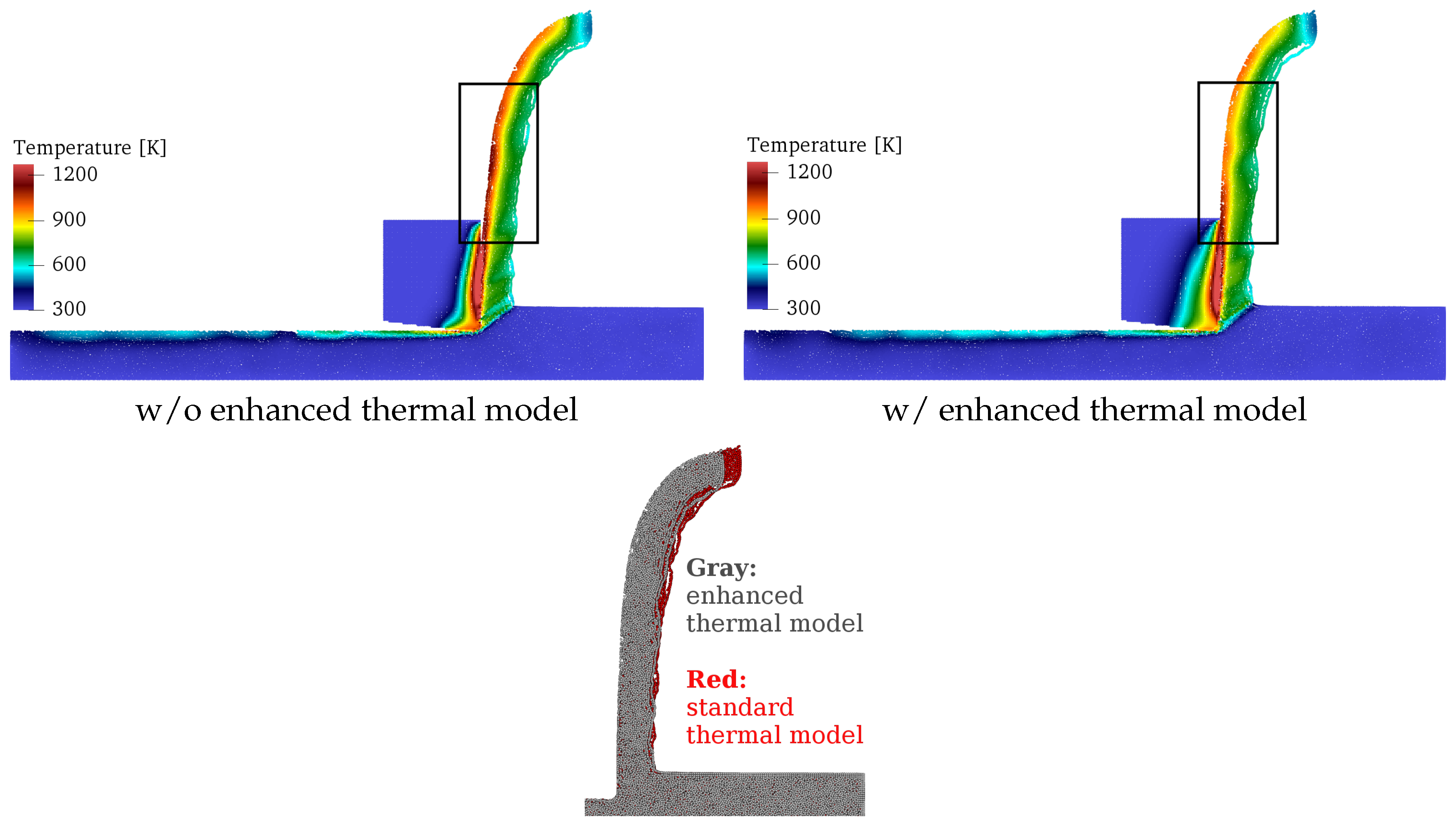
The temperature distribution after $l_c=2$ mm is displayed in Figure 7 to provide some qualitative insights into the thermal aspects of this metal cutting simulation. The left image of this figure is produced by running a simulation with the standard thermal model expressed in Equation (12), where no heat loss boundary condition is included. The middle image in Figure 7 is the result of a simulation including the proposed enhancements outlined in Equations (8) and (13). The chip temperature computed by the enhanced model is slightly lower than the standard model. This is because the open boundaries in the standard thermal model are perfectly isolated and the surface heat loss is ignored. More fundamentally, the essence of this marginal difference between the temperature distributions in Figure 7 can be associated with the constitutive modeling parameters and thermo-physical aspects of Ti6Al4V. To better show the impact of the enhanced thermal model on simulation results, therefore, cutting experiments at lower speeds and/or materials with higher thermal conductivity (e.g., AISI 1045) need to be considered. It is conjectured that running high-resolution SPH simulation of cutting chip formation can also help improve this issue.

Next, the chip shapes of these two models are superimposed with two solid colors for a visual comparison. Ignoring the heat loss boundary condition by the standard model (i.e., the red particles in Figure 7) is the source of slightly more chip curling compared to the present enhanced model (i.e., the gray particles in Figure 7). Clearly, the chip becomes hotter when heat is not lost through its open surfaces.

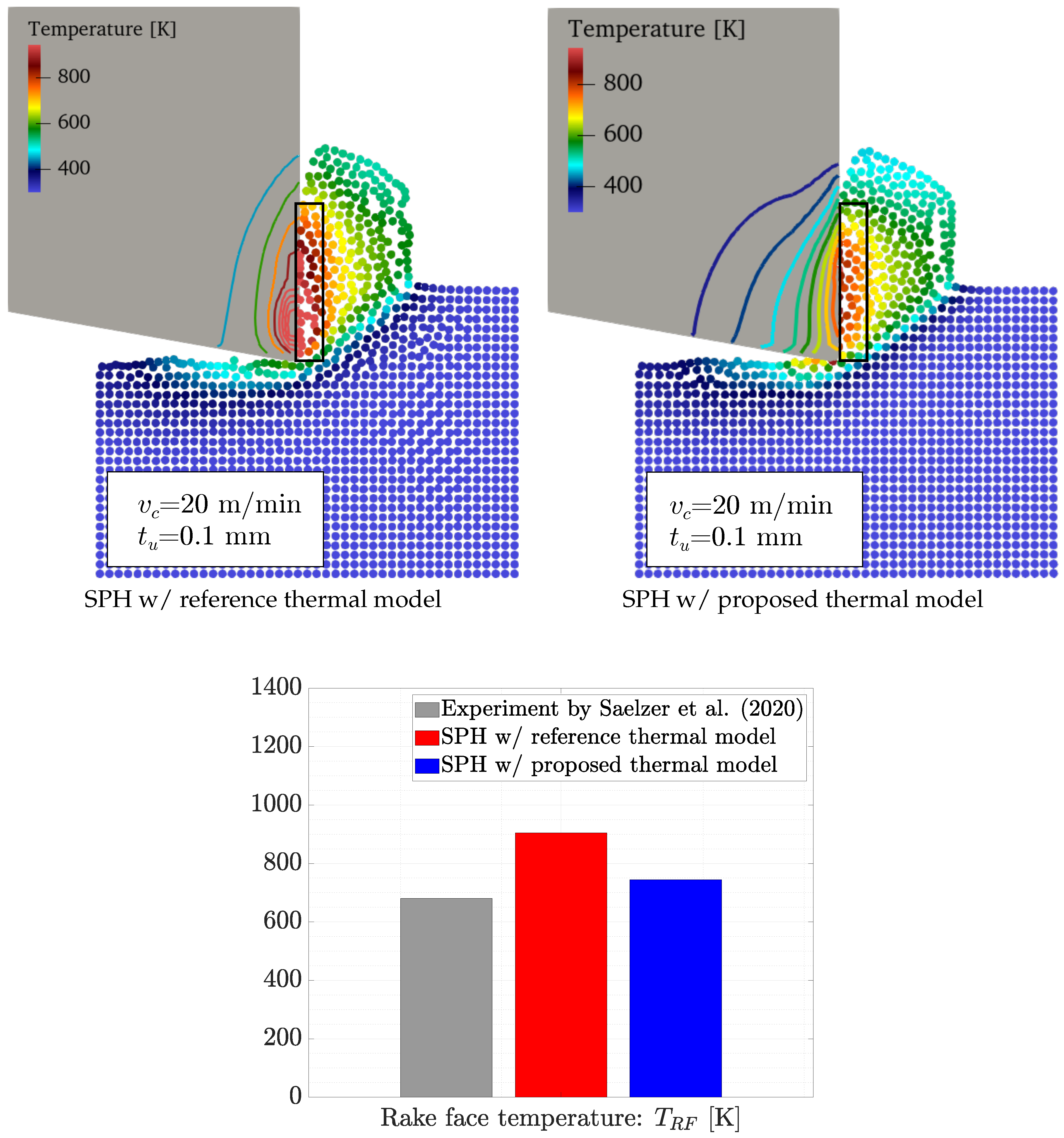
The thermal model in metal cutting has an indirect effect on force prediction, while its impact on the temperature field is direct, and perhaps more significant. Therefore, it is beneficial to demonstrate the improvements gained by the proposed model via a quantitative comparison. For this purpose, an orthogonal cutting experiment conducted by Saelzer et al. [41] is taken into account, where temperature measurements are available. The case study pertains to machining a Ti6Al4V workpiece at a cutting speed of $v_c=20$ m/min, an uncut chip thickness of $t_u=0.1$ mm, and a rake angle of $\gamma =0$°. The rake face temperature ($T_{\mathrm{RF}}$) in this setting is about 680 K. Please note that $v_c=20$ m/min is the lowest speed available in [41], deliberately chosen here to provide more time for thermal conduction in the chip formation zone. As the runtime associated with this relatively low cutting speed is almost 16× longer than the previous test at $v_c=318.5$ m/min, these SPH simulations are carried out at a lower resolution and terminated after a cut distance of $l_c=0.3$ mm.

Shown in Figure 8 are the SPH results employing different thermal models, as well as a comparison of the rake face temperatures. The bar chart in this figure compares the predicted temperatures with the experimentally measured data from [41], which can, in turn, verify the correctness of the proposed thermal model. The red and blue bars are the arithmetic mean temperature of particles located inside the indicated black frames at the rake face, corresponding to 905 K and 744 K, respectively. Using the enhanced thermal model decreases the overprediction error of $T_{\mathrm{RF}}$ from 33% to 9% and leads to a more accurate simulation. This improvement is gained by the more realistic thermal boundary conditions in the proposed model and the utilization of a higher-order Laplacian operator.

5.2.3. Effect of SPH Particles Size

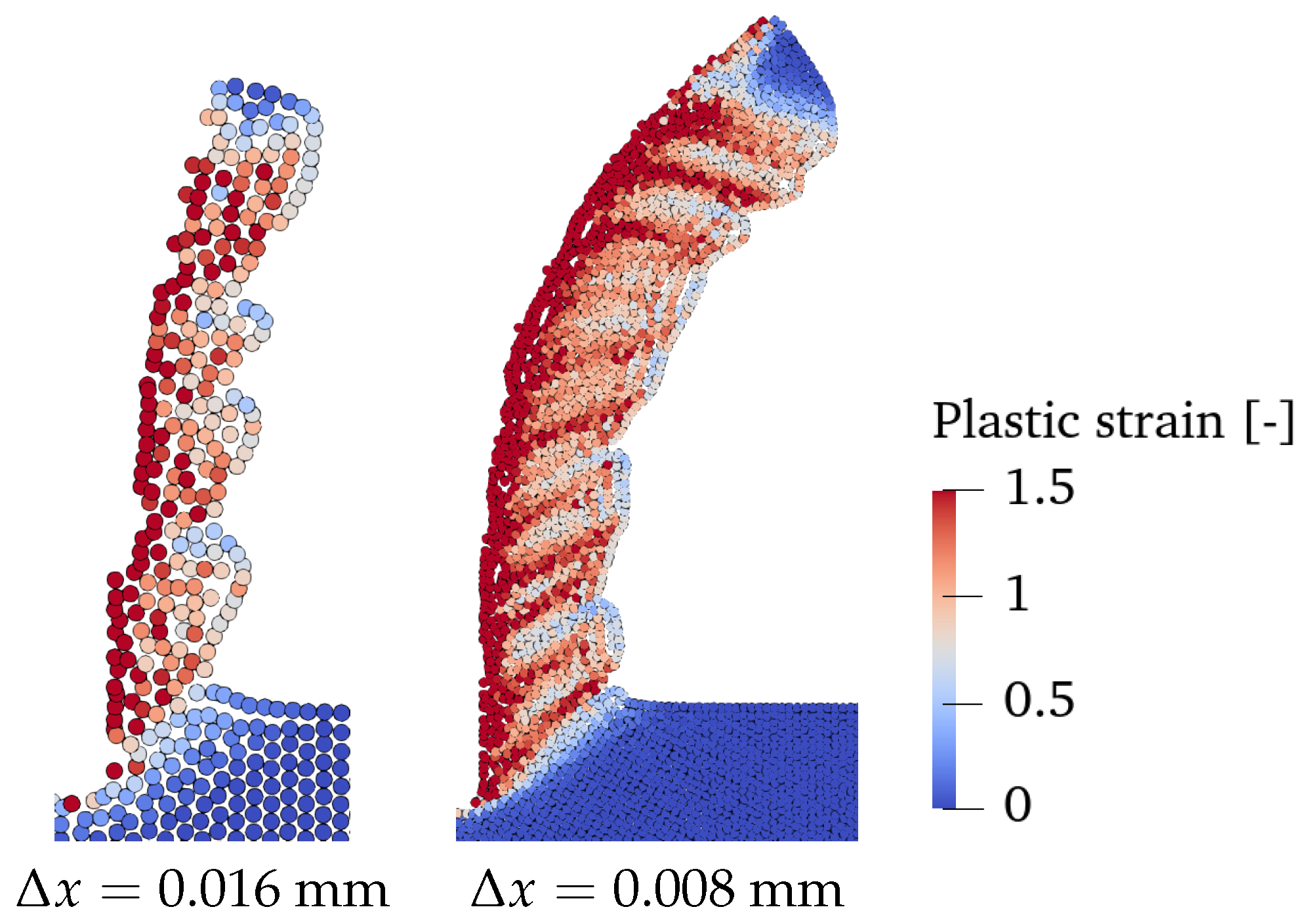
Before closing this section, the effect of resolution (i.e., the size of SPH particles) on the accuracy of the model is briefly discussed. For this purpose, a cutting geometry with $\mu =0.65$ and the parameters listed in Table 1 is considered. Figure 9 shows the equivalent plastic strain distribution for two similar simulations in different resolutions. As seen in this comparison, the high-resolution model (i.e., $\Delta x=0.008$ mm) performs better in capturing the shear bands and chip curling. It can be concluded that reducing the size of SPH particles increases the accuracy of the predicted chip shape.

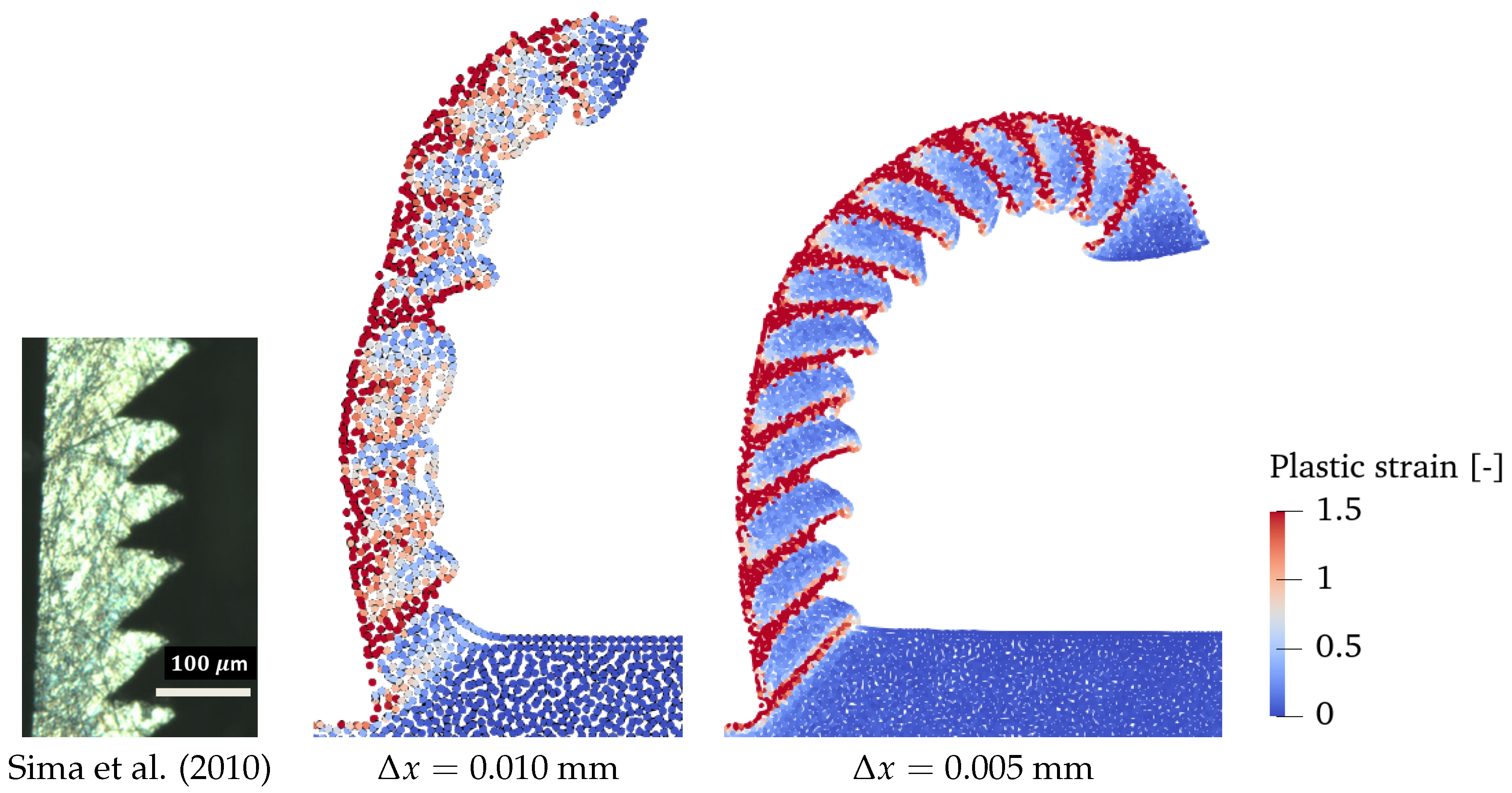
Previous studies have also investigated the influence of discretization size on SPH metal cutting results. For instance, the authors of [20] focused on this subject and presented a new framework for SPH metal cutting models with variable particle size. They showed that the size of SPH particles has a significant impact on the predicted chip shapes. Figure 10 demonstrates this finding, where the chip shape produced by smaller size SPH particles (i.e., the high-resolution case with $\Delta x=0.005$ mm) is much closer to the serrated chip shape observed in the experiment. This, in turn, serves as a qualitative measure of convergence of the method for chip prediction.

6. Conclusions

This paper presented a stabilized SPH framework for numerical simulation of orthogonal metal cutting with an enhanced thermal model. The numerical analysis consists of both thermal and mechanical effects by solving the heat equation in the whole system and considering the elasto-plastic behavior of the material. We found the agreement between the forces measured in the experiment and those predicted by SPH satisfactory, where the average error of force prediction (in both $F_c$ and $F_t$) was smaller than 14% by comparing the numerical and experimental results. It was also shown that the temperature values obtained from the SPH simulation agree with the experimental measurement, leading to more accurate results with the proposed thermal model. The main contributions of this work to the SPH cutting models are summarized in the following.

-

To account for the heat loss boundary condition in SPH cutting models, a new approach was proposed and subsequently applied to an orthogonal cutting problem. This approach incorporates an efficient surface detection algorithm, which was initially proposed for fluid flow applications [5]. An improved thermal model representing more realistic boundary conditions was presented as a result of this development. In addition to the constant temperature at fixed boundaries, heat loss in the forms of thermal convection and radiation was included.

-

To ensure a second-order Laplacian operator in SPH, a corrected formulation (see the FMFS scheme in Equation (13)) was implemented for the first time in a metal cutting problem. This higher-order method allows us to solve the heat equation more accurately, especially in the presence of free surfaces.

Future work opportunities can go in different directions. First, it would be necessary to conduct more experiments for temperature measurements in high-speed cutting. Another enhancement to this study, and perhaps applicable to much of the simulation literature, is determining all material and friction data by a unified numerical-experimental investigation (instead of assuming them from other work). Furthermore, the computational performance of the code needs to be enhanced by high-performance and parallel computing. This consideration is essential for high-resolution simulations of chipping and the 3D implementation of the present code.

References

- Gingold, R.A.; Monaghan, J.J. Smoothed particle hydrodynamics: Theory and application to non-spherical stars. Mon. Not. R. Astron. Soc. 1977, 181, 375–389. [Google Scholar] [CrossRef]
- Lucy, L.B. A numerical approach to the testing of the fission hypothesis. Astron. J. 1977, 82, 1013–1024. [Google Scholar] [CrossRef]
- Monaghan, J.; Kos, A.; Issa, N. Fluid motion generated by impact. J. Waterw. Port Coast. Ocean Eng. 2003, 129, 250–259. [Google Scholar] [CrossRef]
- Afrasiabi, M.; Mohammadi, S. Analysis of bubble pulsations of underwater explosions by the smoothed particle hydrodynamics method. In Proceedings of the ECCOMAS International Conference on Particle Based Methods, Barcelona, Spain, 25–27 November 2009. [Google Scholar]
- Marrone, S.; Colagrossi, A.; Le Touzé, D.; Graziani, G. Fast free-surface detection and level-set function definition in SPH solvers. J. Comput. Phys. 2010, 229, 3652–3663. [Google Scholar] [CrossRef]
- Afrasiabi, M.; Roethlin, M.; Wegener, K. Thermal simulation in multiphase incompressible flows using coupled meshfree and particle level set methods. Comput. Methods Appl. Mech. Eng. 2018, 336, 667–694. [Google Scholar] [CrossRef]
- Afrasiabi, M.; Roethlin, M.; Chatzi, E.; Wegener, K. A Robust Particle-Based Solver for Modeling Heat Transfer in Multiphase Flows. In Proceedings of the European Conference on Computational Mechanics and Computational Fluid Dynamics (ECCM-ECFD), Glasgow, UK, 11–15 June 2018. [Google Scholar]
- Afrasiabi, M.; Chatzi, E.; Wegener, K. A Particle Strength Exchange Method for Metal Removal in Laser Drilling. Procedia CIRP 2018, 72, 1548–1553. [Google Scholar] [CrossRef]
- Afrasiabi, M.; Wegener, K. 3D Thermal Simulation of a Laser Drilling Process with Meshfree Methods. J. Manuf. Mater. Process. 2020, 4, 58. [Google Scholar] [CrossRef]
- Alshaer, A.; Rogers, B.; Li, L. Smoothed Particle Hydrodynamics (SPH) modelling of transient heat transfer in pulsed laser ablation of Al and associated free-surface problems. Comput. Mater. Sci. 2017, 127, 161–179. [Google Scholar] [CrossRef]
- Limido, J.; Espinosa, C.; Salaün, M.; Lacome, J.L. SPH method applied to high speed cutting modelling. Int. J. Mech. Sci. 2007, 49, 898–908. [Google Scholar] [CrossRef] [Green Version]
- Villumsen, M.F.; Fauerholdt, T.G. Simulation of metal cutting using smooth particle hydrodynamics. In Proceedings of the German LS-DYNA Forum 2018, Bamberg, Germany, 15–17 October 2008; pp. C-III-17–C-III-36. [Google Scholar]
- Ruttimann, N.; Buhl, S.; Wegener, K. Simulation of single grain cutting using SPH method. J. Mach. Eng. 2010, 10, 17–29. [Google Scholar]
- Eberhard, P.; Gaugele, T. Simulation of cutting processes using mesh-free Lagrangian particle methods. Comput. Mech. 2013, 51, 261–278. [Google Scholar] [CrossRef]
- Spreng, F.; Eberhard, P. Machining process simulations with smoothed particle hydrodynamics. Procedia CIRP 2015, 31, 94–99. [Google Scholar] [CrossRef] [Green Version]
- Shaw, M.C. Metal Cutting Principles; Oxford University Press: New York, NY, USA, 2005; Volume 2. [Google Scholar]
- Röthlin, M.; Klippel, H.; Afrasiabi, M.; Wegener, K. Metal cutting simulations using smoothed particle hydrodynamics on the GPU. Int. J. Adv. Manuf. Technol. 2019, 102, 3445–3457. [Google Scholar] [CrossRef]
- Roethlin, M.; Klippel, H.; Afrasiabi, M.; Wegener, K. Meshless single grain cutting simulations on the GPU. Int. J. Mechatron. Manuf. Syst. 2019, 12, 272–297. [Google Scholar] [CrossRef]
- Afrasiabi, M.; Meier, L.; Röthlin, M.; Klippel, H.; Wegener, K. GPU-accelerated meshfree simulations for parameter identification of a friction model in metal machining. Int. J. Mech. Sci. 2020, 176, 105571. [Google Scholar] [CrossRef]
- Afrasiabi, M.; Roethlin, M.; Klippel, H.; Wegener, K. Meshfree simulation of metal cutting: An updated Lagrangian approach with dynamic refinement. Int. J. Mech. Sci. 2019, 160, 451–466. [Google Scholar] [CrossRef]
- Fatehi, R.; Manzari, M. Error estimation in smoothed particle hydrodynamics and a new scheme for second derivatives. Comput. Math. Appl. 2011, 61, 482–498. [Google Scholar] [CrossRef]
- Afrasiabi, M.; Roethlin, M.; Wegener, K. Contemporary Meshfree Methods for Three Dimensional Heat Conduction Problems. Arch. Comput. Methods Eng. 2020, 27, 1413–1447. [Google Scholar] [CrossRef]
- Issa, M.; Saanouni, K.; Labergère, C.; Rassineux, A. Prediction of serrated chip formation in orthogonal metal cutting by advanced adaptive 2D numerical methodology. Int. J. Mach. Mach. Mater. 2011, 9, 295–315. [Google Scholar] [CrossRef]
- Taylor, G.I.; Quinney, H. The latent energy remaining in a metal after cold working. Proc. R. Soc. Lond. A 1934, 143, 307–326. [Google Scholar]
- Johnson, G.R. A constitutive model and data for materials subjected to large strains, high strain rates, and high temperatures. In Proceedings of the Seventh International Symposium on Ballistics, The Hague, The Netherlands, 19–21 April 1983; pp. 541–547. [Google Scholar]
- Özel, T. The influence of friction models on finite element simulations of machining. Int. J. Mach. Tools Manuf. 2006, 46, 518–530. [Google Scholar] [CrossRef]
- Liu, M.; Liu, G. Smoothed particle hydrodynamics (SPH): An overview and recent developments. Arch. Comput. Methods Eng. 2010, 17, 25–76. [Google Scholar] [CrossRef] [Green Version]
- Monaghan, J.J. Smoothed particle hydrodynamics. Rep. Prog. Phys. 2005, 68, 1703. [Google Scholar] [CrossRef]
- Monaghan, J.J. Smoothed particle hydrodynamics. Annu. Rev. Astron. Astrophys. 1992, 30, 543–574. [Google Scholar] [CrossRef]
- Brookshaw, L. A method of calculating radiative heat diffusion in particle simulations. Proc. Astron. Soc. Aust. 1985, 6, 207–210. [Google Scholar] [CrossRef]
- Deligonul, Z.; Bilgen, S. Solution of the Volterra equation of renewal theory with the Galerkin technique using cubic splines. J. Stat. Comput. Simul. 1984, 20, 37–45. [Google Scholar] [CrossRef]
- Monaghan, J.; Gingold, R. Shock simulation by the particle method SPH. J. Comput. Phys. 1983, 52, 374–389. [Google Scholar] [CrossRef]
- Gray, J.; Monaghan, J.; Swift, R. SPH elastic dynamics. Comput. Methods Appl. Mech. Eng. 2001, 190, 6641–6662. [Google Scholar] [CrossRef]
- Monaghan, J. On the problem of penetration in particle methods. J. Comput. Phys. 1989, 82, 1–15. [Google Scholar] [CrossRef]
- Afrasiabi, M. Thermomechanical Simulation of Manufacturing Processes Using GPU-Accelerated Particle Methods. Ph.D. Thesis, ETH Zurich, Zurich, Switzerland, 2020. [Google Scholar] [CrossRef]
- Randles, P.; Libersky, L. Smoothed particle hydrodynamics: Some recent improvements and applications. Comput. Methods Appl. Mech. Eng. 1996, 139, 375–408. [Google Scholar] [CrossRef]
- Arrazola, P.; Özel, T.; Umbrello, D.; Davies, M.; Jawahir, I. Recent advances in modelling of metal machining processes. CIRP Ann.-Manuf. Technol. 2013, 62, 695–718. [Google Scholar] [CrossRef]
- Stöcker, H. Taschenbuch der Physik; In Deutsch: Zurich, Switzerland, 2000. [Google Scholar]
- Niu, W.; Mo, R.; Liu, G.; Sun, H.; Dong, X.; Wang, G. Modeling of orthogonal cutting process of A2024-T351 with an improved SPH method. Int. J. Adv. Manuf. Technol. 2018, 95, 905–919. [Google Scholar] [CrossRef]
- Ducobu, F.; Rivière-Lorphèvre, E.; Filippi, E. On the importance of the choice of the parameters of the Johnson-Cook constitutive model and their influence on the results of a Ti6Al4V orthogonal cutting model. Int. J. Mech. Sci. 2017, 122, 143–155. [Google Scholar] [CrossRef]
- Saelzer, J.; Berger, S.; Iovkov, I.; Zabel, A.; Biermann, D. In-situ measurement of rake face temperatures in orthogonal cutting. CIRP Ann. 2020, 69, 61–64. [Google Scholar] [CrossRef]
- Sima, M.; Özel, T. Modified material constitutive models for serrated chip formation simulations and experimental validation in machining of titanium alloy Ti–6Al–4V. Int. J. Mach. Tools Manuf. 2010, 50, 943–960. [Google Scholar] [CrossRef]
Figure 1.
Illustration of heat sources and thermal boundary conditions in orthogonal cutting.
Figure 2.
Illustration of the proposed approach for thermal boundary conditions. Left: introduction of the surface detection algorithm into SPH cutting models. The implementation considers the tool (rigid) and the workpiece (deformable) as two separate bodies. Right: only particles with are included and then categorized into 2 surface groups (red and blue). Thermal boundary conditions are imposed on these blue and red surface particles accordingly.
Figure 3.
Reconstruction of the Laplacian operator acting on a 2D quadratic function.
Figure 4.
Configuration of orthogonal metal cutting problem and a closeup of the force diagram.
Figure 5.
Evolution of predicted forces compared to the experimental data.
Figure 6.
Summary of the measured and predicted forces for the cutting test. Forces predicted by SPH with different coefficients of friction are plotted in the bar chart, where the proposed thermal model is utilized. Impact of on the thrust forces is higher than the cutting forces, demonstrating the most accurate result when is used.
Figure 7.
Distribution of the temperature after 2 mm of cut. Lower temperatures are observed in the enhanced model by comparing the two black frames. Simulated chip shapes are superimposed to give insights into the impact of the heat loss boundary condition on chip curling.
Figure 8.
Distributions and contours of temperature obtained by SPH using the reference and proposed thermal model. An average of the rake face temperature in simulation results (considering the particles inside the black frames) is compared to the experimental measurement provided by [41]. The color bar is limited to 945 K for better visibility.
Figure 9.
Effect of SPH particles size on the chip shape, where is the diameter of SPH particles.
Figure 10.
Comparison of chip shapes in different SPH resolutions, where m/min, mm, and mm. The experimental photograph reprinted from Sima et al. [42] Copyright (2021), with permission from Elsevier under License Number 4991260002261.