Image Anomaly Detection Using Normal Data Only by Latent Space Resampling

Abstract

Detecting image anomalies automatically in industrial scenarios can improve economic efficiency, but the scarcity of anomalous samples increases the challenge of the task. Recently, autoencoder has been widely used in image anomaly detection without using anomalous images during training. However, it is hard to determine the proper dimensionality of the latent space, and it often leads to unwanted reconstructions of the anomalous parts. To solve this problem, we propose a novel method based on the autoencoder. In this method, the latent space of the autoencoder is estimated using a discrete probability model. With the estimated probability model, the anomalous components in the latent space can be well excluded and undesirable reconstruction of the anomalous parts can be avoided. Specifically, we first adopt VQ-VAE as the reconstruction model to get a discrete latent space of normal samples. Then, PixelSail, a deep autoregressive model, is used to estimate the probability model of the discrete latent space. In the detection stage, the autoregressive model will determine the parts that deviate from the normal distribution in the input latent space. Then, the deviation code will be resampled from the normal distribution and decoded to yield a restored image, which is closest to the anomaly input. The anomaly is then detected by comparing the difference between the restored image and the anomaly image. Our proposed method is evaluated on the high-resolution industrial inspection image datasets MVTec AD which consist of 15 categories. The results show that the AUROC of the model improves by 15% over autoencoder and also yields competitive performance compared with state-of-the-art methods.

1. Introduction

One of the key factors in optimizing the manufacturing process is automatic anomaly detection, which makes it possible to prevent production errors, thereby improving quality and bringing economic benefits to the plant. The common practice of anomaly detection in industry is for a machine to make judgments on images acquired through digital cameras or sensors. This is essentially an image anomaly detection problem that is looking for patterns that are different from normal images [1]. Humans can easily handle this task through awareness of normal patterns, but this is relatively difficult for machines. Unlike other computer vision tasks, image anomaly detection suffers from some of the following inevitable challenges: class imbalance, variety of anomaly types, and unknown anomaly [2,3]. Anomalous instances are generally rare, whereas normal instances account for a significant proportion. In addition, distinct and even unknown types can be exhibited in anomalies such as varied sizes, shapes, locations, or textures. Therefore, it is almost impossible to capture a large number of abnormal data containing all anomaly types. Many methods are instead designed in a semi-supervised way, using only normal images as training samples.

Some methods usually consider the anomaly detection problem as a “one-class” problem that initially models the normal data as background and then evaluates whether the test data belong to this background or not, by the degree of difference from the background [4]. In the early applications of surface defect detection, the background is often modeled by designing handmade features on defect-free data. For example, Bennatnoun et al. [5] adopt texture primitives called blobs [6] to uniquely characterize the flawless texture and to detect defects through changes in the attributes of blobs. Amet et al. [7] use wavelet filters to obtain subband images of defect-free samples, then extract the co-occurrence features of subband images, from which a classifier is trained to defect detection. However, most of these methods focus on textures that are periodic and monotonic while less valid for randomly natural textures.

Recently, deep learning techniques have been widely used in computer vision related tasks. It can automatically extract hierarchical features from the data and learn rich semantic representations, avoiding the need for manual feature development. Deep generative models as a sub-domain of deep learning techniques can model data distribution. AutoEncoder including its variants (AEs) is an important branch, as it has a unique reconstruction property that is widely used in anomaly detection tasks. AEs can map the input data nonlinearly into a low-dimensional latent space and reconstruct back into the data space. These models are trained in an unsupervised way by minimizing input and output errors. Some work [8,9,10,11] exploits the characteristics of AEs to use only normal images during training in an attempt to restrict the latent space dimension and capture the manifold of normal images. They assume that this will result in AEs failing to reconstruct well during prediction due to anomalous images deviating from the normal manifold. These works use reconstruction errors as scores for identifying anomalies with larger meaning more likely to be anomalies. However, AEs are originally designed for reconstruction, whose performance to be tightly coupled with the size of the latent space [12]. With no knowledge of the essential dimension of the data, setting the dimension of the latent space too small or too large would cause potential problems for AE-based anomaly detection methods. A large setting may result in undetectable anomalies caused by good reconstruction of anomalous images, and conversely may result in false detection of normal as abnormal. We propose a method to circumvent the above problems by adopting an AE-like model with strong reconstruction performance for the purpose of reducing false detections. To solve the problem that anomalies can also be reconstructed caused by excessive reconstruction capability, we introduce a deep autoregressive (DAR) model. By using DAR to constrain the latent space of the anomalous image in the distribution of normal images, AE can reconstruct the normal sample closest to the corresponding anomalous image. Based on this framework, we also propose a novel anomaly score to further improve anomaly detection, which exploits the residuals of both reconstructions with and without latent space constraints. We use VQ-VAE [13] applied to the compression task as the reconstruction model for the proposed method, with VQ-VAE providing a discrete latent space that can improve the modeling efficiency of DAR. For the DAR model, as PixelSNAIL [14] can generate an image by modeling a joint distribution of pixels as well as giving the likelihood of each pixel, we use it as the tool to constrain the distribution of latent space. The proposed method is evaluated on the large-scale real-world industrial image dataset MVTec AD [15] and compared it with several major anomaly detection methods. The experiments show that our method yields better performance compared with the state of the art.

The main contributions of this paper are as follows:

• We propose a novel method only using normal data for image anomaly detection. It effectively excludes the anomalous components in the latent space and avoids the unwanted reconstruction of the anomalous part, which achieves better detection results.
• We propose a new method for anomaly score. The high anomaly scores are concentrated in the regions where anomalies are present, which will reduce the noise introduced by the reconstruction and improve precision.

The remainder of this paper is organized as follows: Section 2 reviews the related work of image anomaly detection. A detailed description of our proposed method is given in Section 3. Section 4 presents experimental setups and comparisons. The conclusion is finally summarized in Section 5.

2. Related Work

There exists an abundance of work on image anomaly detection over the last several decades, and we outline several types of methods related to the proposed approach.

2.1. Feature Extraction Based Method

Feature extraction-based methods generally map images to the appropriate feature space and detect anomalies based on distance. Generally, feature extraction and anomaly detection are disjointed. Abdel-Qader et al. [16] proposed a PCA-based method for concrete bridge deck crack detection. They first use PCA to get dominant eigenvectors of tested image patches and then calculate the European distance from the dominant eigenvectors of normal image patches. Liu et al. [17] used SVDD to detect defects in TFT-LCD array images. They described an image patch with four features including entropy, energy, contrast, and homogeneity and trained an SVDD model using normal image patches. If a feature vector lies outside the hypersphere found by SVDD during testing, the image patch corresponding to this feature vector is considered anomalous. Similar works can be found in [18,19,20]. Compared to these traditional dimensionality reduction models, a convolutional neural network (CNN) provides nonlinear mapping and is better at extracting semantic information. There are two common practices for applying CNN for feature extraction, one is to use a pre-trained network, such as VGG or ResNet, and the other is to develop a deep feature extraction model specifically for the purpose. For example, Napoletano et al. [21] used a pre-trained ResNet-18 to extract feature vectors from the scanning electron microscope (SEM) images to construct a dictionary. In the prediction phase, a tested image is considered anomalous if the average Euclidean distance between its feature and its m nearest neighbors in the dictionary is higher than the threshold. The other is the Deep SVDD model developed by Ruff et al. [22] who combine CNN with SVDD. They trained the deep neural network by minimizing the volume of the hypersphere containing feature vectors of the data.

2.2. Probability Based Method

These methods assume that anomalies occur in low probability regions of the normal data, and the main principle is as follows: (i) Establish the probability density function (PDF) of normal data; (ii) Evaluate the test samples by PDF and low probability density values are most likely to be abnormal. There are various methods depending on the distribution assumptions, such as Gaussian [23], Gaussian Mixture Model (GMM) [24] or Markov random fields (MRF) [25]. For instance, Böttger et al. [26] improved on the framework of [23], they applied the CS theory [27] to compress defect-free texture patches into texture features and use GMM to estimate their probability distributions. In the detection stage, a pixel is considered to be defective if the likelihood of the local patch corresponding to it is less than the threshold value. Recently deep learning methods have improved PDF estimation performance. Due to the powerful image generation capability of deep autoregressive (DAR) model, it is also used for anomaly detection. Richter et al. [28] applied PixelCNN [29] to circuit board images that predicted pixel likelihood to anomaly detection, but it may not work well in more complex natural images. One advantage of the DAR model is that it can give the likelihood for each pixel, but Shafaei et al. [30] recently compared several anomaly detection methods, whose anomaly scores are given as softmax output, Euclidean distance, likelihood, etc. The experimental results show that PixelCNN++ using likelihood as the anomaly score has a lower accuracy than the mean. This shows that it is unsuitable to use low likelihood values as the anomaly score directly. Our method combines the advantages of DAR, using likelihood for resampling instead of scoring directly. On the other hand, we use DAR to estimate density for a low-dimensional discrete latent space, which avoids the problem of “curse of dimensionality” to improve modeling efficiency.

2.3. Reconstruction Based Method

The assumption of this kind of method is that normal images can be reconstructed from latent space better than anomalous images. Early defect detection works utilized sparse dictionary [31,32] for reconstruction. Deep learning techniques have extended the toolbox of reconstruction-based methods. Autoencoder-like models are the commonly-used model for these kinds of methods. Generally, AE-like based methods can be summarized as (i) training AE from only normal samples; and (ii) anomaly segmentation based on reconstruction error of input samples, which may have anomalies. Baur et al. [10] applied AE directly to detect pathologies in Brain MR Images. In particular, VAE attempts to detect anomalies through the generated perspective. Some work [8,11] assumes that VAE trained on normal images will only be able to reconstruct normal images, thus getting larger reconstruction errors in anomalous regions. Since the essential dimensions of the data are not known, information may be lost after a bottleneck and even normal parts may not be reconstructed correctly, resulting in false detections. Several approaches have been proposed to address this issue. Bergmann et al. [9] thought ${\ell }^p$-distance would enlarge slightly reconstruction errors and replaced it with SSIM. Nair et al. [33] are the first to use uncertainty estimate based on Monte Carlo dropout for lesion detection. They perform dropout operation on AE and then take the variance of result as anomaly score. Both Venkataramanan et al. [34] and Liu et al. [35] implemented Grad-CAM [36] into AE, aiming to replace reconstruction errors with the attention mechanism and achieving outstanding performance. Haselmann et al. [37] treated anomaly detection as an inpainting problem that uses AE trained on the normal dataset to generate patches clipped on the image. Dehaene et al. [38] argued that learning only on normal manifold does not guarantee generalization outside of the manifold, which will lead to unreliable reconstruction. They used iterative energy-based projection to sample the closest normal image to the anomalous input on normal manifold. Another is to apply Generative adversarial networks (GAN), and Schlegl et al. [39] used GAN to model normal OCT images of retina distribution. At the time of the prediction, searching the latent space for suitable latent codes makes the generator yield the normal sample closest to the anomalous input, and then use ${\ell }^1$ distance as anomaly score. Soon after, Schlegl et al. [40] optimized the search process before the generator. Similarly, GANomaly [41] adds GAN’s discriminator to AE and encodes the reconstructed image for detecting the anomalies in X-ray images by summing the errors of latent code, reconstruction error, and adversarial loss as anomaly scores. However, GAN suffers from pattern collapse that may yield plausible samples and cause false alarms.

3. Method

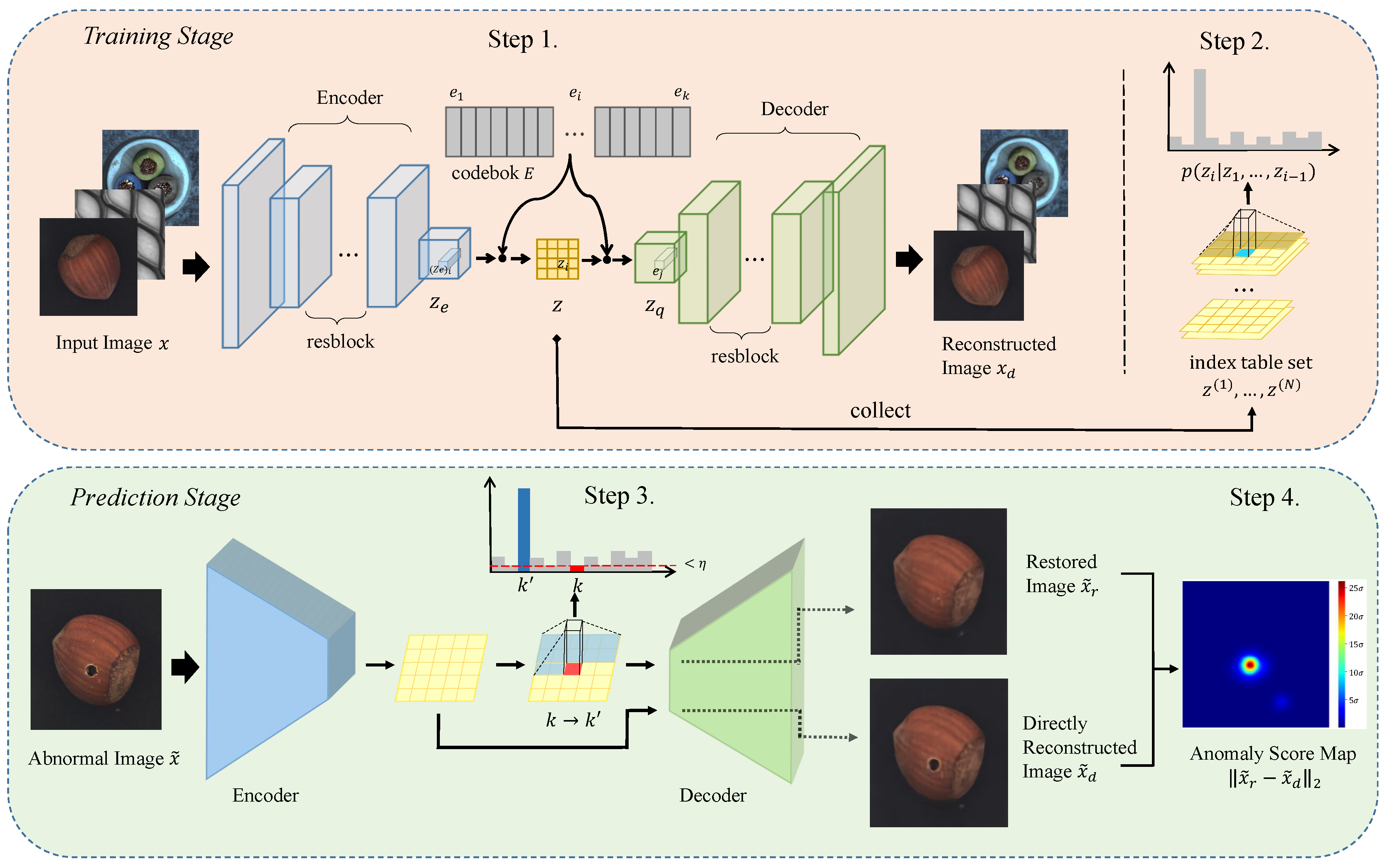
This section describes the principles of our proposed method. The first step is to train a VQ-VAE using anomaly-free images as training data. When VQ-VAE can embed anomaly-free images into a compact discrete latent space and reconstruct high-quality outputs, we start performing the second step. All anomaly-free images are first encoded using the trained VQ-VAE to collect a latent code set, and then the probability distribution of this latent code set is estimated using PixelSNAIL. At the prediction stage, when the latent code of an input image is out of the distribution learned in the second step, PaxielSNAIL will conduct resampling operations on it. The resampled latent code is decoded as a restored image, which is used for anomaly detection by calculating the error with the directly reconstructed image. The overall work-flow of the proposed method is shown in Figure 1; in the following, we describe it in detail.

3.1. Structuring Latent Space

VQ-VAE is originally proposed as a compression model with good results, and we use it as a reconstruction model to construct the latent space. It is different from VAE; VAE assumes that the latent space satisfies a Gaussian prior and reconstructs using the re-parameterization trick, which implies that the process of getting the latent representation is indeterministic. However, VQ-VAE encodes the input to the latent representation with a deterministic mapping and reconstructs data from quantized vectors. VQ-VAE provides a sufficiently large latent space dimension, resulting in far better reconstruction performance than VAE and AE. Since the latent space is discrete, it can be modeled by deep autoregressive models, and the estimated probability distribution is the basis for the proposed resampling operation.

VQ-VAE consists of an encoder, a codebook with K embedding vectors $\mathbf{e}\in {\mathbb{R}}^{K\times D}$, and a decoder. The method trains discrete latent variables $\mathbf{z}\in {\mathbb{R}}^{M\times N}$ using the codebook combined with nearest neighbor search, which is performed on the encoder output ${\mathbf{z}}_{\mathbf{e}}\in {\mathbb{R}}^{M\times N\times D}$ using the ${\ell }^2$-distance. Then, the vectors in the codebook replace ${\mathbf{z}}_{\mathbf{e}}$ to yield ${\mathbf{z}}_{\mathbf{q}}\in {\mathbb{R}}^{M\times N\times D}$ as input to the decoder, where $\mathbf{z}$ is used as the index table for ${\mathbf{z}}_{\mathbf{e}}$ transformation to ${\mathbf{z}}_{\mathbf{q}}$. The model optimizes the parameters of the encoder, decoder, and codebook, with the goal of minimum reconstruction errors.

Specifically, as shown in step 1 in Figure 1, given an anomaly-free input image x, the encoder first encodes x into $M\times N$ D-dimensional vectors $z_e$ that maintain the two-dimensional spatial structure of the image. These vectors are then quantized based on their nearest distance to the embedding vectors $e_{1,2,...,k}$ in the codebook; the process can be defined by Equation (1):

$$z_i=\underset{j\in \{1,\cdots ,K\}}{argmin}{∥{\left(z_e\right)}_i-e_j∥}_2$$

(1)

This quantization process is essentially a lookup process, resulting in an index table z. The index table maintains the same spatial structure as $z_e$, whose value for each component is the sequence number of embedding vectors in the codebook. Each vector in $z_e$ will be replaced by the e nearest to it before decoding, where e is selected directly in the codebook based on the value of the corresponding position in z, as shown in Equation (2):

$${\left(z_q\right)}_i=e_{z_i}$$

(2)

Finally, the decoder maps this replaced vectors $z_q$ back to the image $x_d$. With the quantization operation, the discrete $\mathbf{z}$ can represent the whole latent space, and thus changing the value of $\mathbf{z}$ at prediction stage can generate the desired reconstructed images.

To learn these mappings, we randomly initialize $e_{1,2,...,k}$ by sampling in the Gaussian distribution $N(0,1)$ before training and through the loss function described in Equation (3) to train the model, where $sg[·]$ operation represents equality in forward propagation and zero derivative in backward propagation:

$$\mathcal{L}=\parallel \mathbf{x}-{\mathbf{x}}_{\mathbf{d}}{\parallel }_2+\parallel sg\left[{\mathbf{z}}_{\mathbf{e}}\right]-{\mathbf{z}}_{\mathbf{q}}{\parallel }_2+\beta {\parallel {\mathbf{z}}_{\mathbf{e}}-sg\left[{\mathbf{z}}_{\mathbf{q}}\right]\parallel }_2$$

(3)

The entire loss function has three components. The first term is reconstruction loss, which encourages the output to be as close to the input as possible. The second term is used to constrain the embedding vectors in the codebook, minimizing the loss of information caused by replacing ${\mathbf{z}}_{\mathbf{e}}$ with ${\mathbf{z}}_{\mathbf{q}}$. Before computing this term, indices of the nearest embedding vectors to ${\mathbf{z}}_{\mathbf{e}}$ are computed, and then ${\mathbf{z}}_{\mathbf{q}}$ is composed based on the index lookup. To prevent ${\mathbf{z}}_{\mathbf{e}}$ from fluctuating too frequently, the final term is used to normalize ${\mathbf{z}}_{\mathbf{e}}$. During training, ${\mathbf{z}}_{\mathbf{e}}$ is required to guarantee the quality of the reconstruction, and ${\mathbf{z}}_{\mathbf{q}}$ is relatively free. A weight factor $\beta$ is set with the expectation that “let ${\mathbf{z}}_{\mathbf{q}}$ go closer to ${\mathbf{z}}_{\mathbf{e}}$” more than “let ${\mathbf{z}}_{\mathbf{e}}$ go closer to ${\mathbf{z}}_{\mathbf{q}}$”.

3.2. Probabilistic Modeling for Latent Space

In order to constrain the latent space, a distribution of the latent space of normal images needs to be estimated. Deep autoregressive models allow for stable, parallel, and easy-to-optimize density estimation of sequence data. Another advantage is the ability to provide data likelihood, which makes our anomaly detection possible. PixelCNN [29] was one of the first autoregressive models implemented using convolutional neural networks applied to image generation, and many improved models have been developed based on it. Here, we use PixelSNAIL [14], an enhanced version of PixelCNN that adds the Self-Attention mechanism [42] to model long-term dependencies.

To estimate the probability distribution of the image, PixelSNAIL transforms the joint distribution of all pixels into a product of chain probabilities as shown in Equation (4). Each pixel is modeled as a conditional distribution, indicating the current pixel value is determined by all pixels preceding it:

$$p\left(\mathbf{x}\right)=p\left(x_1,\dots ,x_n\right)=\prod _{i=1}^{n}p\left(x_i\mid x_1,\dots ,x_{i-1}\right)$$

(4)

The conditional distribution $p\left(x_i\mid x_{<i}\right)$ is parameterized by a convolutional neural network and finally connected to a softmax layer to estimate the probability of 256 values. Mask convolution is used to guarantee the conditional relationship preventing the model from reading pixels below. The whole training process can be parallelized using the GPU.

When the VQ-VAE training is completed, as shown in step 2 in Figure 1, we extract the index table set $\left\{z^{\left(1\right)},z^{\left(2\right)},\dots ,z^{\left(N\right)}\right\}$ by encoding all N normal images. For any $z^{\left(i\right)}$ in the index table set, since it records only the index of the embedded vector in the codebook, one can treat it as a single-channel image. Each “pixel” in the index table has K possible values, depending on the size of the codebook.

The process of modeling the probability distribution of the index table by PixelSNAIL is analogous to the process for a low-resolution image as described above. The network is trained using the cross-entropy loss function with the expectation that the inference of the network will be identical to the true index. After training, the network can capture the pattern of normal images in latent space, predicting the most likely current index number based on the preceding index order.

3.3. Resampling Operation

VQ-VAE’s powerful reconstruction capability implies that it also has strong generalization capability. During the prediction stage, unseen anomalous images are encoded whose latent codes deviate from the distribution of normal images, and this caused values in index tables to change as well. Our intention is to reconstruct a normal image that most closely matches the corresponding anomalous image. The word “closest” is achieved by means that only the areas where anomalies exist are restored, while the normal areas remain unchanged. Since the index arrangement of the index table determines the final latent code to be decoded, the restored image can be reconstructed by updating the value in the index table that does not satisfy the normal image pattern.

Specifically, as shown in step 3 of Figure 1, an anomalous image $\tilde{x}$ is pushed into the encoder network and extracted an $M\times N$ index table $\tilde{z}$. Then, the trained PixelSNAIL model infers the likelihood on each component of $\tilde{z}$ in parallel. In this process, PixelSNAIL will estimate the conditional distribution of current component of $\tilde{z}$ based on arrangement characteristics of the preceding. If the component of $\tilde{z}$ is assigned an extremely low likelihood, it means that the index does not conform to the pattern of normal images. We set a hyperparameter threshold $\eta$ to identify these anomalous patterns, and the setting of this threshold is described in detail in the experimental section. When the likelihood of the current component is less than the threshold $\eta$, we perform a resampling operation in the conditional distribution of that component, generating a new index that is most likely to occur under the semantics of the preceding normal pattern. The entire resampling process is carried out in raster order, ensuring that the pre-sequence arrangement follows the normal images’ pattern.

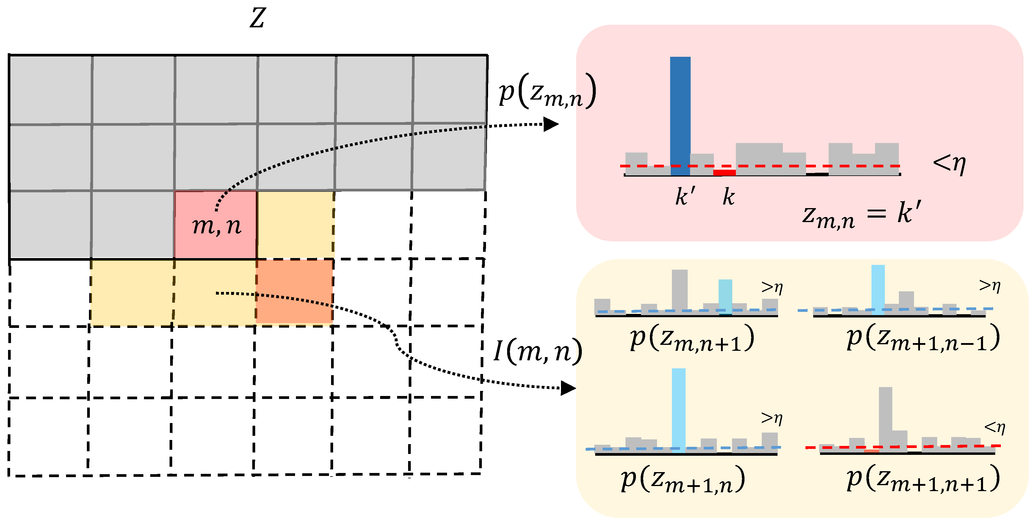
The resampling operation can be defined by Equation (5), where $I(m,n)$ means the minimum conditional probability given the bottom half of the 8-neighbor of ${\tilde{z}}_{m,n}$, $1<m,n<M,N$:

$${\tilde{z}}_{m,n}=\left\{\begin{array}{cc}\underset{k^{\prime }\in \{1,\cdots ,K\}}{argmax}p(Z_{m,n}=k^{\prime }\mid {\tilde{z}}_{i,j<m,n})\hfill & \mathrm{if}p\left(Z_{m,n}=k\mid {\tilde{z}}_{i,j<m,n}\right)<\eta \mathrm{and}I(m,n)<\eta \hfill \\ k\hfill & \mathrm{others}\hfill \end{array}\right.$$

(5)

We assume that anomalous region usually has local continuity, and, based on this assumption, we add a local constraint $I(m,n)<\eta$ to increase the stability of the resampling. As Figure 2 shows, the probability distribution of the current component (red zone) is conditioned only on previous sequences, lacking the semantic information underneath it. We introduce the likelihood about the bottom half (yellow zone) of the current component’s 8-neighbor to avoid noise. Resampling operation is applied when the likelihood of both current component and at least one component in the bottom half is less than the threshold.

3.4. Detection of Anomalies

Based on indexes recorded in the resampled index table, the corresponding embedding vectors can be extracted from the codebook to yield the normal quantized latent code. After that, the decoder maps this quantized latent code back to the image space to reconstruct the restored image ${\tilde{x}}_r$. Reconstruction-based methods typically calculate the reconstruction error of the input and output the anomaly score, with higher scores representing more likely anomalies. However, we chose the ${\ell }^2$-distance between the VQ-VAE directly reconstructed image ${\tilde{x}}_d$ and the restored image ${\tilde{x}}_r$ which is defined in Equation (6), as the anomaly score to perform anomaly detection:

$$\mathcal{A}(i,j)={∥{\tilde{x}}_r(i,j)-{\tilde{x}}_d(i,j)∥}_2$$

(6)

We argue that the VQ-VAE model is applied to compression, the reconstruction may only lose some details, but the semantics of the raw image is not changed. In addition, anomalies are typically small in both size and proportion to the image being processed [1], and VQ-VAE has enough generalization capability to reconstruct these unseen anomalies. As resampling operation is applied only to components with very low likelihood values in the index table, the results calculated using Equation (6) will only have high anomaly scores in certain regions, reducing the possibility of false alarms. We verified the proposed anomaly score in the experimental section, and the results also show that ours is better than using traditional detection methods.

After getting the residual map, we apply a smoothing post-processing using bilateral filtering. The smoothed anomaly score map shows the anomaly score for each pixel, and the final segmentation can be obtained by binarization operation to identify the location of the anomaly.

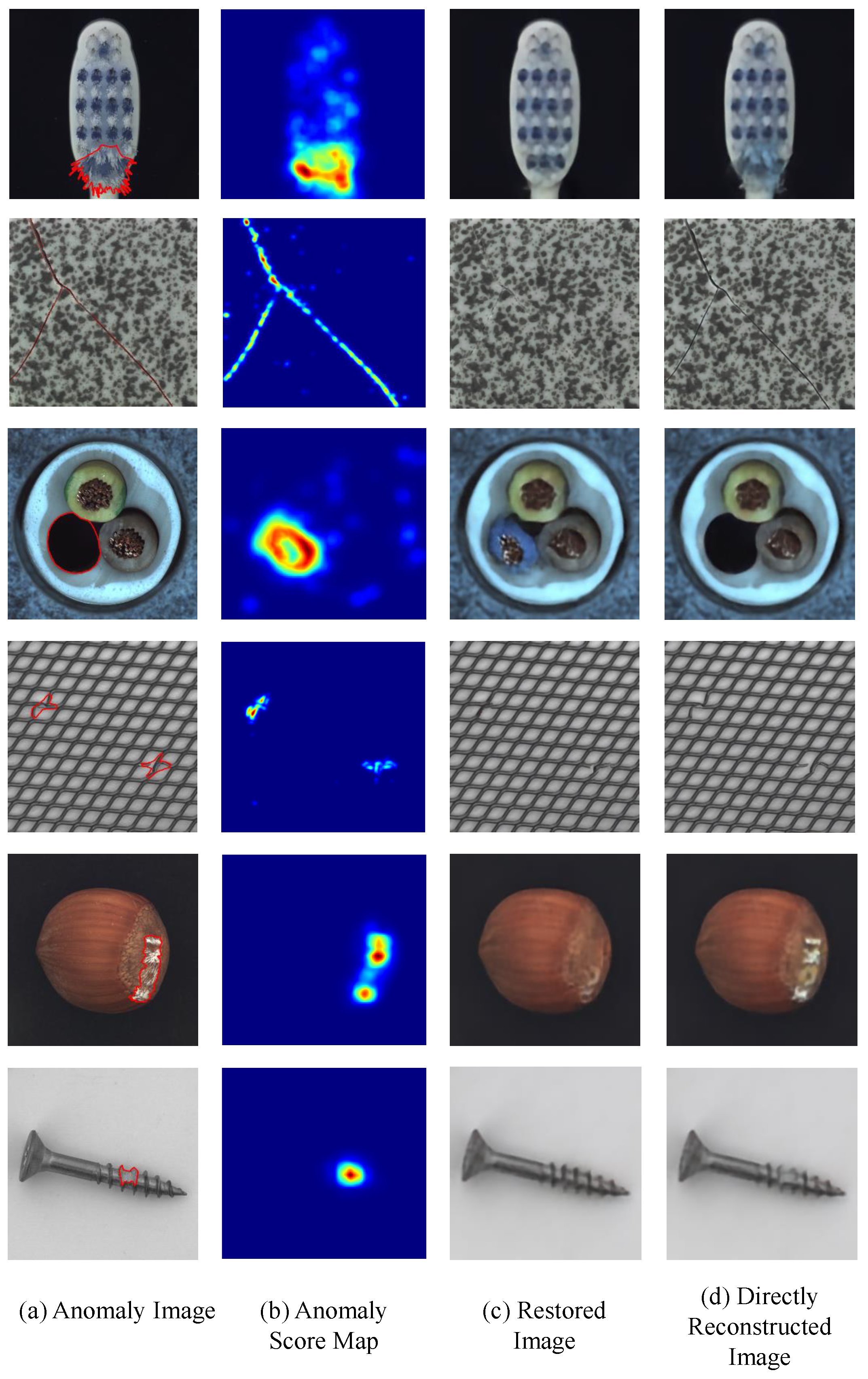
Some visual examples of the above process are given in Figure 3. Since images are mapped to a unified latent space that is quantized as a discrete and solidified codebook, PixelSNAIL can easily determine whether to resample from the distribution of normal images based on a fixed threshold, followed by the decoder generating an anomaly-free sample closest to the input. Figure 3c shows restored images decoded from resampled index tables. Comparing with the original images in Figure 3a, one can see that the decoder only regenerates for the parts that have anomalies, but not for the whole image. As shown in Figure 3d, VQ-VAE can still reconstruct unseen anomalies, maintaining the structure of the original images. By comparing these two reconstructed images, it is possible to obtain areas that are considered anomalous as shown in Figure 3b.

4. Experiment

Our experiments were designed to detect anomalies in images. We used the MVTec AD dataset for evaluation. In this section, we first describe the composition of the dataset and some training settings. Secondly, the detection performance of the proposed model is verified by comparing it with other methods. Thirdly, we performed ablation experiments to demonstrate the effects of the proposed anomaly score and the local constraint.

4.1. Dataset

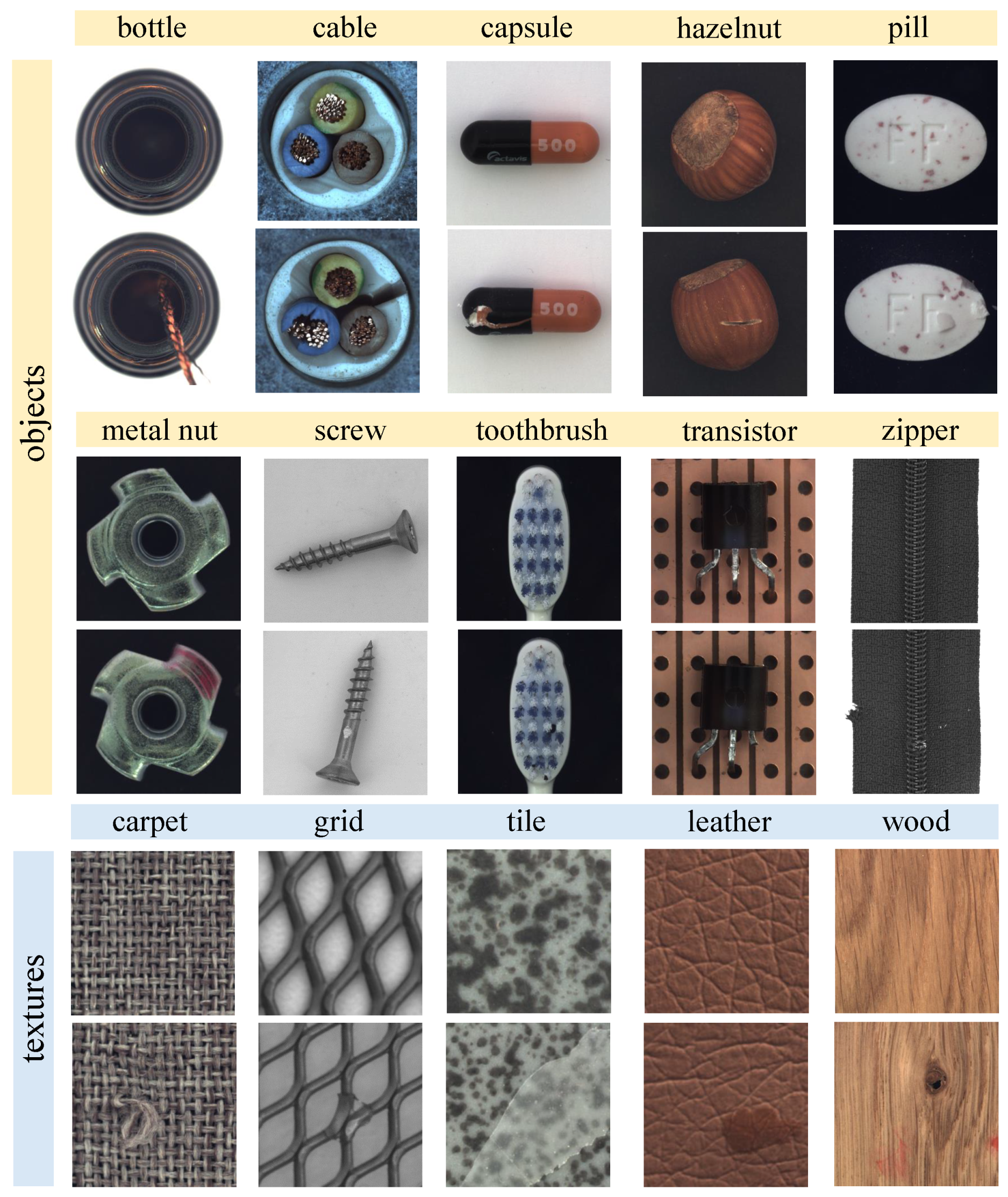
We evaluate the performance of the proposed method on the comprehensive natural image anomaly detection dataset: MVTec AD dataset [15]. The MVTec AD dataset provides over 5000 high-resolution images divided into five texture and 10 object categories. Texture types cover both regular (carpet, grid) and random (leather, tile, wood) cases, while the remaining 10 objects contain rigid, fixed appearance (bottle, metal nut), deformable (cable), and natural variation (hazelnut) cases. The dataset configures a scenario that only provides normal images during training. For each class, the training set is only composed of anomaly-free images, and the test set consists of anomaly-free images as well as images containing 73 different types of fine-grained anomalies, such as defects on the objects’ surface like scratches or dents, structural defects like distortion of object parts, or defects due to the missing parts of certain objects. Pixel-precise ground truth labels are provided for each anomaly image region. The dataset overview is shown in Figure 4. The MVTec AD dataset can be downloaded in https://www.mvtec.com/company/research/datasets/mvtec-ad/.

4.2. Evaluation Metric

We use the same evaluation criteria defined in Bergmann et al. [15] to test the proposed method’s performance. First, a minimum area of connected components is set for each category. Then, using the method to be evaluated to predict anomaly score maps on a validation set containing only normal images. After that, binary decisions are made on these anomaly score maps by incremental thresholds. Until the area of the largest connected component in binary images is equal to the defined minimum area, this threshold is determined as the final binary threshold. Based on this threshold, we calculate the average of the percentage of correct images that are correctly classified as anomaly-free and anomaly for image-level detection. For pixel-level detection, evaluate per-region overlap (PRO) and the area under the ROC curve (AUROC). PRO is the relative per-region overlap of the predicted segmentation map $S_p$ with the ground truth $S_g$, and it gives greater weight to the connectivity component that contains fewer pixels:

$$PRO=\frac{1}{n}\sum _i^n\frac{s_p^{\left(i\right)}}{s_g^{\left(i\right)}}$$

(7)

where $s_p^{\left(i\right)},s_g^{\left(i\right)},n$ are each connected component of $S_p$ and its corresponding $S_g$ and the number of connected components it contains, respectively. In addition, the image-level and pixel-level F1 Score are also evaluated, where F1 score is computed as:

$$Recall=\frac{TP}{TP+FN}$$

(8)

$$Precision=\frac{TP}{TP+FP}$$

(9)

$$F1Score=\frac{2·Precision·Recall}{Precision+Recall}$$

(10)

We define TP as the count of images or pixels correctly classified as anomalous, FP as the count of images or pixels incorrectly classified as anomalous, and FN as the count of images or pixels incorrectly classified as normal.

4.3. Experimental Setup

The experimental environment is a computer with Intel Xeon E5-2667 CPU, 64 GB of RAM, Nvidia 1080ti GPU, running Ubuntu 18.04, and we use the Pytorch library to implement our architecture.

4.3.1. Data Augmentation

To diversify the training set to make the model more generalizable, we use random transforms and rotations on the MVTec AD dataset to augment the training data. Specifically, applying random rotation selected from a set $\left\{0^{\circ },{90}^{\circ },{180}^{\circ },{270}^{\circ }\right\}$ and random flip to texture categories and some object categories (bottle, hazelnut, metal nut, and screw). The remaining object categories are randomly rotated between the range $\left[-{10}^{\circ },{10}^{\circ }\right]$. Finally, all categories are rescaled to $256\times 256$, where texture categories are achieved by random cropping.

4.3.2. Network Setup

For VQ-VAE parameter configuration, the encoder is implemented as six convolutional layers with kernel size 4, stride step 2, padding 1, and followed by ReLU, one convolutional layer with kernel size 3, stride step 1, padding 1 and followed by eight residual blocks, which are implemented as ReLU, $3\times 3$ conv, ReLU, $1\times 1$ conv for each block. Images are encoded as $z_e$ with shape $32\times 32\times 32$. The decoder is a symmetrical structure of the encoder using transposed convolutions. The dimensionality of the codebook and z are designed as $512\times 32$ ($K=512$) and $32\times 32$, respectively. The weight factor $\beta$ is set to $0.25$. We use the ADAM optimizer with learning rate 3e-4 and train for 100 epochs with batch size 256. For PixelSNAIL parameter configuration, the model consists of one residual block and one attention block, both of which are repeated three times due to the limitations of GPU memory trained for 150 epochs with batch size 64, ADAM optimizer, and learning rate 0.0003. We set the parameters d, color sigma, and space sigma of the bilateral filter to (20,75,75).

4.3.3. Hyperparameter Setup

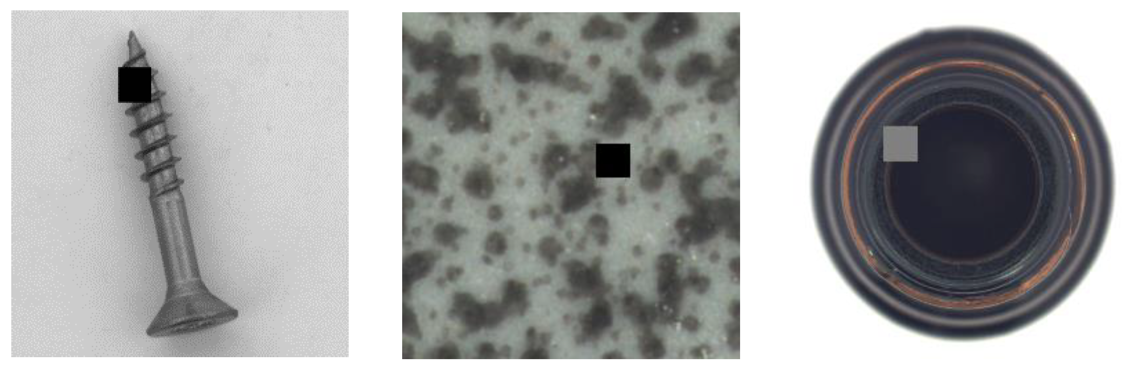
To determine the hyperparameter $\eta$, we make a validation set containing negative samples shown in Figure 5 and performed a grid search on this validation set until reaching the maximum AUROC. We randomly mask the anomaly-free images with black or gray rectangles that are $1\%$ of the size of the prototype to generate negative samples. In the experiment, we set $0.0005$ as the value of $\eta$.

4.4. Comparison Results

We present separately the results calculated according to the three different evaluation metrics and compared with the baseline methods listed in Bergmann et al. [15] as well as with other recent related methods to evaluate the performance of the proposed method.

Table 1. The average of accuracy of correctly classified anomalous images and anomaly-free images on the MVTec AD dataset. Red is optimal.

	Category	Proposed	CAVGA-$D_{\mathit{u}}$ [34]	${\mathrm{AE}}_{\mathit{SSIM}}$ [9]	${\mathrm{AE}}_{\mathit{L}\mathit{2}}$ [9]	AnoGAN [39]	CNNFD [21]	TI [26]
Textures	Carpet	0.71	0.73	0.67	0.50	0.49	0.63	0.59
	Grid	0.91	0.75	0.69	0.78	0.51	0.67	0.50
	Wood	0.96	0.85	0.83	0.74	0.68	0.84	0.71
	Leather	0.96	0.71	0.46	0.44	0.52	0.67	0.50
	Tile	0.95	0.70	0.52	0.77	0.51	0.71	0.72
Objects	Bottle	0.99	0.89	0.88	0.80	0.69	0.53	-
	Cable	0.72	0.63	0.61	0.56	0.53	0.61	-
	Capsule	0.68	0.83	0.61	0.62	0.58	0.41	-
	Hazelnut	0.94	0.84	0.54	0.88	0.50	0.49	-
	Metal Nut	0.83	0.67	0.54	0.73	0.50	0.65	-
	Pill	0.68	0.88	0.60	0.62	0.62	0.46	-
	Screw	0.80	0.77	0.51	0.69	0.35	0.43	-
	Toothbrush	0.92	0.91	0.74	0.98	0.57	0.57	-
	Transistor	0.73	0.73	0.52	0.71	0.67	0.58	-
	Zipper	0.97	0.87	0.80	0.80	0.59	0.54	-
	mean	0.85	0.78	0.63	0.71	0.55	0.59	0.60

shows the average accuracy of correctly classified anomalous and normal images, which demonstrates the ability of the method in the image-level classification task. Our proposed method yields better classification results in 10 of the 15 categories, with improvements ranging from $1\%$ to $35\%$. It is not as good as ${\mathrm{CAVGA}-\mathrm{D}}_u$ [34] in both pill and capsule categories due to some anomalies similar to the normal random fine-grained pattern like spots that make the distinction more difficult, but the results are still superior to the baseline method.

Table 2. The per-region overlap (PRO) on the MVTec AD dataset. Red is optimal.

	Category	Proposed	CAVGA-$D_{\mathit{u}}$ [34]	VAE with Attention [35]	${\mathrm{AE}}_{\mathit{SSIM}}$ [9]	${\mathrm{AE}}_{\mathit{L}\mathit{2}}$ [9]	AnoGAN [39]	CNNFD [21]
Textures	Carpet	0.47	0.71	0.10	0.69	0.38	0.34	0.20
	Grid	0.89	0.32	0.02	0.88	0.83	0.04	0.02
	Wood	0.53	0.56	0.14	0.36	0.29	0.14	0.47
	Leather	0.80	0.76	0.24	0.71	0.67	0.34	0.74
	Tile	0.36	0.31	0.23	0.04	0.23	0.08	0.14
Objects	Bottle	0.52	0.30	0.27	0.15	0.22	0.05	0.07
	Cable	0.40	0.37	0.18	0.01	0.05	0.01	0.13
	Capsule	0.31	0.25	0.11	0.09	0.11	0.04	0.00
	Hazelnut	0.54	0.44	0.44	0.00	0.41	0.02	0.00
	Metal Nut	0.36	0.39	0.49	0.01	0.26	0.00	0.13
	Pill	0.24	0.34	0.18	0.07	0.25	0.17	0.00
	Screw	0.47	0.42	0.17	0.03	0.34	0.01	0.00
	Toothbrush	0.69	0.54	0.14	0.08	0.51	0.07	0.00
	Transistor	0.08	0.30	0.30	0.01	0.22	0.08	0.03
	Zipper	0.82	0.20	0.06	0.10	0.13	0.01	0.00
	mean	0.50	0.41	0.20	0.22	0.33	0.09	0.13

and

Table 3. The AUROC on the MVTec AD dataset. Red is optimal.

	Category	Proposed	VAE with Attention [35]	${\mathrm{AE}}_{\mathit{SSIM}}$ [9]	${\mathrm{AE}}_{\mathit{L}\mathit{2}}$ [9]	AnoGAN [39]	CNNFD [21]
Textures	Carpet	0.94	0.78	0.87	0.59	0.54	0.72
	Grid	0.99	0.73	0.94	0.90	0.58	0.59
	Wood	0.87	0.77	0.73	0.73	0.62	0.91
	Leather	0.99	0.95	0.78	0.75	0.64	0.87
	Tile	0.88	0.80	0.59	0.51	0.50	0.93
Objects	Bottle	0.95	0.87	0.93	0.86	0.86	0.78
	Cable	0.95	0.90	0.82	0.86	0.78	0.79
	Capsule	0.93	0.74	0.94	0.88	0.84	0.84
	Hazelnut	0.95	0.98	0.97	0.95	0.87	0.72
	Metal Nut	0.91	0.94	0.89	0.86	0.76	0.82
	Pill	0.95	0.83	0.91	0.85	0.87	0.68
	Screw	0.96	0.97	0.96	0.96	0.80	0.87
	Toothbrush	0.97	0.94	0.92	0.93	0.90	0.77
	Transistor	0.91	0.93	0.90	0.86	0.80	0.66
	Zipper	0.98	0.78	0.88	0.77	0.78	0.76
	mean	0.94	0.86	0.87	0.82	0.74	0.78

show the results of the comparison at the pixel level. Our proposed method is better than other methods as a whole on all metrics. PRO is highly demanding on the segmentation performance of the model under test, and even small areas of anomalous region prediction errors can reduce the value of this metric. We achieve the best results on grid, leather, and zipper, and leading results in the other seven categories as well. It is feasible to restore the anomalous portion of the image by resampling in low-dimensional latent space. Since Venkataramanan et al. [34] does not list specific AUROC, we selected VAE with Attention [35] for comparison. Our results at AUROC were better than the second ${\mathrm{AE}}_{SSIM}$ [9] with an $8\%$ improvement as Table 3 showed. Benefiting from the strong reconstruction capability of VQ-VAE and the constraint of resampling operations, the score of anomalies portion in the image is much larger than the normal portion. This leads to better results than other reconstruction-based methods, which mostly suffer from false detection due to insufficient reconstruction of the normal portion.

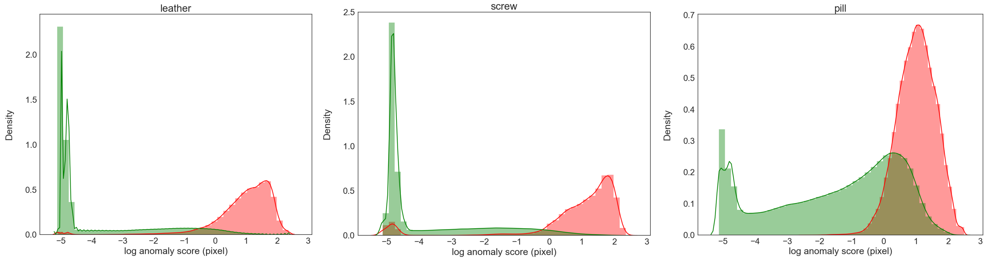
We further calculate the the F1 Score at the image level and pixel level to evaluate the classification and segmentation performance of the model. As shown in

Table 4. The image-level and pixel-level F1 Score on the MVTec AD dataset. The left side of each category is the F1 Score at the image level and the right is the F1 Score at the pixel level.

	Category	Proposed	${\mathrm{AE}}_{\mathit{SSIM}}$ [9]	${\mathrm{AE}}_{\mathit{L}\mathit{2}}$ [9]
Textures	Carpet	0.88/0.33	0.87/0.08	0.54/0.03
	Grid	0.97/0.38	0.90/0.02	0.92/0.04
	Wood	0.97/0.42	0.88/0.12	0.64/0.24
	Leather	0.98/0.42	0.81/0.02	0.76/0.32
	Tile	0.98/0.30	0.09/0.07	0.71/0.07
Objects	Bottle	0.99/0.55	0.92/0.16	0.90/0.26
	Cable	0.82/0.40	0.58/0.02	0.29/0.06
	Capsule	0.68/0.23	0.58/0.08	0.39/0.10
	Hazelnut	0.93/0.50	0.13/0.44	0.89/0.46
	Metal Nut	0.93/0.36	0.15/0.03	0.83/0.25
	Pill	0.81/0.20	0.43/0.09	0.37/0.25
	Screw	0.81/0.34	0.11/0.06	0.56/0.20
	Toothbrush	0.97/0.40	0.80/0.14	0.98/0.35
	Transistor	0.68/0.11	0.06/0.07	0.60/0.19
	Zipper	0.99/0.58	0.75/0.29	0.77/0.15
	mean	0.89/0.37	0.54/0.11	0.68/0.20

, the average result at the image level is $0.89$, showing that the proposed model is basically able to correctly distinguish between anomalous and normal images. For pixel-level classification, since the number of anomalous pixels is much smaller than normal pixels, this can greatly affect the precision and thus indirectly the F1 Score. For example, a screw may have anomalies only in the head, and the number of these anomalous pixels accounts for only 1–2% of the image. When the predicted anomaly area is enlarged a bit, the precision may drop by more than 50%, but the prediction is intuitively acceptable in terms of pixel continuity. Although the metric assigns equal weights to positive and negative classes, we think the proposed model gives relatively good results, with the mean value 0.17 higher than AE-L2. Furthermore, we present the distribution of anomaly score for leather/screw/pill in Figure 6. The proposed model tends to assign high anomaly scores to anomalous pixels and low anomaly scores to normal pixels.

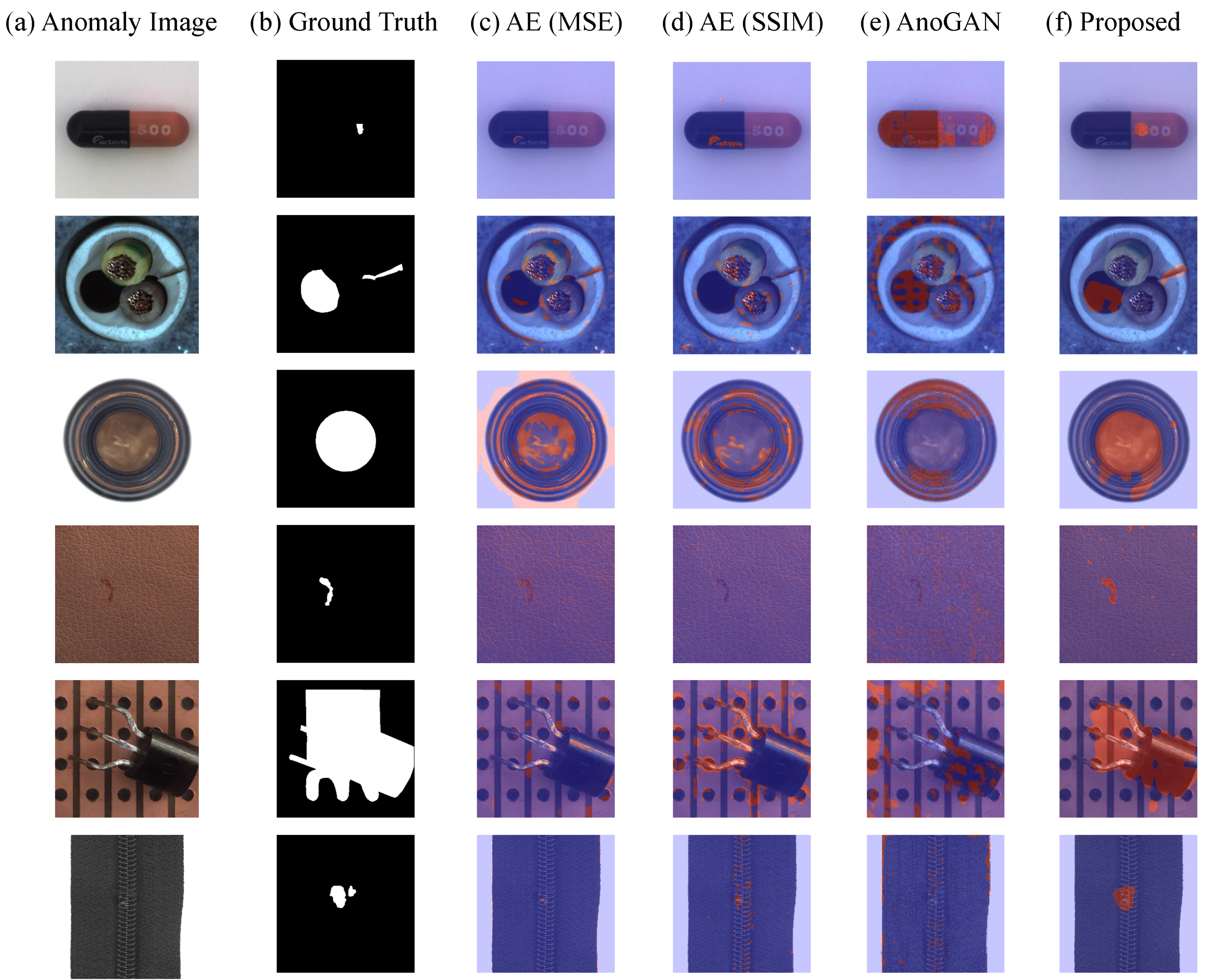
Moreover, we demonstrate some visual comparison results with the baseline methods in Figure 7. These test images contain various anomalies such as missing parts, distorted or scratched parts, misalignment, etc. Our proposed method can correctly detect these different anomalies of varying sizes. In the first row, the print on the capsule is scratched, and AE fails to reconstruct these prints accurately, resulting in high anomaly scores for all prints. The second and fifth rows are the missing anomalous cable and misplaced transistor separately; these two segmentation results illustrate that the proposed method can reconstruct the normal image closest to the anomalous input and thus precisely locate the anomaly. In all of these anomaly types, the segmentation results of the proposed method are roughly the same as ground truth, while the other methods can only detect part of them.

4.5. Ablation Experiment

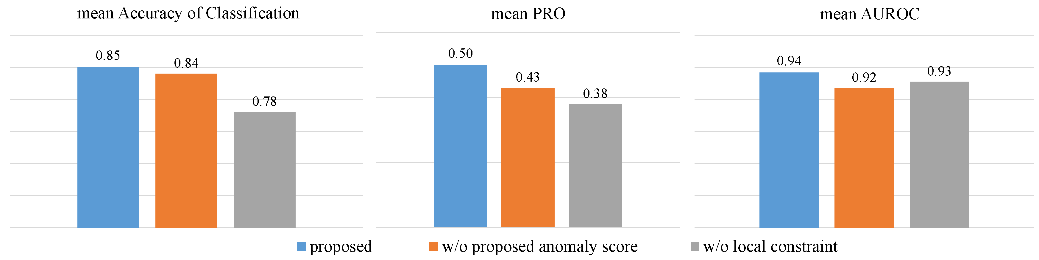
To verify the validity of the proposed anomaly scores and the local constraint on the resampling operation, we performed ablation experiments separately. We use the ${\ell }^2$ distance between input and output to get the anomaly score map and give comparison results with the proposed method. We also compare the model without the local constraint. The averages of the above three metrics are presented in Figure 8. The results show that, when the anomaly score map is binarized obtained from input and output residuals, the threshold needs to be raised to overcome the high anomaly scores in normal regions caused by reconstruction noise, but it also leads to a lower predicted recall yet. The proposed method only has residuals in regions with anomalies, thus providing a higher signal-to-noise ratio and precision.

With the removal of local constraints, the resampling operation may be affected by noise and may even affect the following judgement which leads to lower results. However, models without local constraint are still better on average than the AE model and are competitive with the state-of-the art.

5. Conclusions

Due to the lack of sufficient anomaly data relative to normal data, we introduce a novel method for anomaly detection using only normal data. The work can be summarized as follows:

• Using VQ-VAE to construct a discrete latent space. Then, the latent space distribution of the normal image is modeled using PixelSNAIL.
• During anomaly detection, the discrete latent code out of the normal distribution is resampled by PixelSNAIL. After this resampling, the index table is reconstructed to a restored image by the decoder. The greater the distance between the restored image and the image reconstructed directly using VQ-VAE, the more likely the region is anomalous.
• The method is evaluated on the industrial inspection dataset MVTec AD that contains 10 objects and five textures with 73 various anomalies. The results show that the proposed method achieves better performance compared to other methods.

Our motivation can be intuitively explained as keeping the normal portions intact while restoring the abnormal portions of images. Since the time required for resampling and inference is related to dimension of the latent space, this may constrain real-time performance of our method. In addition, it is possible to collect a small number of anomalous images in reality, and introducing this anomalous information may improve the performance of the model. Future work will focus on real-time performance and semi-supervised learning.

References

- Ehret, T.; Davy, A.; Morel, J.M.; Delbracio, M. Image Anomalies: A Review and Synthesis of Detection Methods. J. Math. Imaging Vis. 2019, 61, 710–743. [Google Scholar] [CrossRef] [Green Version]
- Chalapathy, R.; Chawla, S. Deep learning for anomaly detection: A survey. arXiv 2019, arXiv:1901.03407. [Google Scholar]
- Pang, G.; Shen, C.; Cao, L.; Hengel, A.v.d. Deep Learning for Anomaly Detection: A Review. arXiv 2020, arXiv:2007.02500. [Google Scholar]
- Markou, M.; Singh, S. Novelty detection: A review—Part 1: Statistical approaches. Signal Process. 2003, 83, 2481–2497. [Google Scholar] [CrossRef]
- Bennamoun, M.; Bodnarova, A. Automatic visual inspection and flaw detection in textile materials: Past, present and future. In Proceedings of the IEEE International Conference on Systems, Man, and Cybernetics (SMC), San Diego, CA, USA, 14 October 1998. [Google Scholar] [CrossRef]
- Voorhees, H. Finding Texture Boundaries in Images; Technical Report; Computer Science and Artificial Intelligence Lab (CSAIL): Cambridge, MA, USA, 1987. [Google Scholar]
- Amet, A.L.; Ertuzun, A.; Erçil, A. Texture defect detection using subband domain co-occurrence matrices. In Proceedings of the IEEE Southwest Symposium on Image Analysis and Interpretation (SSIAI), Tucson, AZ, USA, 5–7 April 1998; pp. 205–210. [Google Scholar] [CrossRef]
- Zimmerer, D.; Kohl, S.A.; Petersen, J.; Isensee, F.; Maier-Hein, K.H. Context-encoding variational autoencoder for unsupervised anomaly detection. arXiv 2018, arXiv:1812.05941. [Google Scholar]
- Bergmann, P.; Löwe, S.; Fauser, M.; Sattlegger, D.; Steger, C. Improving Unsupervised Defect Segmentation by Applying Structural Similarity to Autoencoders. In Proceedings of the International Joint Conference on Computer Vision, Imaging and Computer Graphics Theory and Applications (VISIGRAPP), SCITEPRESS, Prague, Czech, 25–27 February 2019. [Google Scholar] [CrossRef]
- Baur, C.; Wiestler, B.; Albarqouni, S.; Navab, N. Deep Autoencoding Models for Unsupervised Anomaly Segmentation in Brain MR Images; International MICCAI Brainlesion Workshop; Springer: Berlin/Heidelberg, Germany, 2018; pp. 161–169. [Google Scholar] [CrossRef] [Green Version]
- An, J.; Cho, S. Variational autoencoder based anomaly detection using reconstruction probability. Spec. Lect. IE 2015, 2, 1–18. [Google Scholar]
- Goodfellow, I.; Bengio, Y.; Courville, A. Deep Learning; MIT Press: Cambridge, MA, USA, 2016; pp. 500–501. [Google Scholar]
- Van Den Oord, A.; Vinyals, O.; Kavukcuoglu, K. Neural discrete representation learning. In Proceedings of the Neural Information Processing Systems (NIPS), Long Beach, CA, USA, 4–9 December 2017; pp. 6306–6315. [Google Scholar]
- Chen, X.; Mishra, N.; Rohaninejad, M.; Abbeel, P. Pixelsnail: An improved autoregressive generative model. In Proceedings of the International Conference on Machine Learning (ICML), Stockholmsmässan, Stockholm, Sweden, 10–15 July 2018. [Google Scholar]
- Bergmann, P.; Fauser, M.; Sattlegger, D.; Steger, C. MVTec AD—A Comprehensive Real-World Dataset for Unsupervised Anomaly Detection. In Proceedings of the IEEE/CVF Conference on Computer Vision and Pattern Recognition (CVPR), Long Beach, CA, USA, 16–20 June 2019. [Google Scholar] [CrossRef]
- Abdel-Qader, I.; Pashaie-Rad, S.; Abudayyeh, O.; Yehia, S. PCA-Based algorithm for unsupervised bridge crack detection. Adv. Eng. Softw. 2006, 37, 771–778. [Google Scholar] [CrossRef]
- Liu, Y.H.; Lin, S.H.; Hsueh, Y.L.; Lee, M.J. Automatic target defect identification for TFT-LCD array process inspection using kernel FCM-based fuzzy SVDD ensemble. Expert Syst. Appl. 2009, 36, 1978–1998. [Google Scholar] [CrossRef]
- Tout, K.; Cogranne, R.; Retraint, F. Fully automatic detection of anomalies on wheels surface using an adaptive accurate model and hypothesis testing theory. In Proceedings of the European Signal Processing Conference (EUSIPCO), Budapest, Hungary, 29 August–2 September 2016. [Google Scholar] [CrossRef]
- Mao, T.; Ren, L.; Yuan, F.; Li, C.; Zhang, L.; Zhang, M.; Chen, Y. Defect Recognition Method Based on HOG and SVM for Drone Inspection Images of Power Transmission Line. In Proceedings of the International Conference on High Performance Big Data and Intelligent Systems (HPBD&IS), Shenzhen, China, 9–11 May 2019. [Google Scholar] [CrossRef]
- Liu, K.; Wang, H.; Chen, H.; Qu, E.; Tian, Y.; Sun, H. Steel Surface Defect Detection Using a New Haar–Weibull-Variance Model in Unsupervised Manner. IEEE Trans. Instrum. Meas. 2017, 66, 2585–2596. [Google Scholar] [CrossRef]
- Napoletano, P.; Piccoli, F.; Schettini, R. Anomaly detection in nanofibrous materials by cnn-based self-similarity. Sensors 2018, 18, 209. [Google Scholar] [CrossRef] [Green Version]
- Ruff, L.; Görnitz, N.; Deecke, L.; Siddiqui, S.; Vandermeulen, R.A.; Binder, A.; Müller, E.; Kloft, M. Deep One-Class Classification. In Proceedings of the International Conference on Machine Learning (ICML), Stockholmsmässan, Stockholm, Sweden, 10–15 July 2018. [Google Scholar]
- Du, B.; Zhang, L. Random-Selection-Based Anomaly Detector for Hyperspectral Imagery. IEEE Trans. Geosci. Remote Sens. 2011, 49, 1578–1589. [Google Scholar] [CrossRef]
- Xie, X.; Mirmehdi, M. TEXEMS: Texture Exemplars for Defect Detection on Random Textured Surfaces. IEEE Trans. Pattern Anal. Mach. Intell. 2007, 29, 1454–1464. [Google Scholar] [CrossRef] [PubMed] [Green Version]
- Ozdemir, S.; Ercil, A. Markov random fields and Karhunen-Loeve transforms for defect inspection of textile products. In Proceedings of the IEEE Conference on Emerging Technologies and Factory Automation, (ETFA), Kauai, HI, USA, 18–21 November 1996. [Google Scholar] [CrossRef]
- Böttger, T.; Ulrich, M. Real-time texture error detection on textured surfaces with compressed sensing. Pattern Recognit. Image Anal. 2016, 26, 88–94. [Google Scholar] [CrossRef]
- Candès, E.; Tao, T. Decoding by linear programming. IEEE Trans. Inf. Theory 2005, 51, 4203–4215. [Google Scholar] [CrossRef] [Green Version]
- Richter, J.; Streitferdt, D. Deep Learning Based Fault Correction in 3D Measurements of Printed Circuit Boards. In Proceedings of the IEEE Annual Information Technology, Electronics and Mobile Communication Conference (IEMCON), UBC, Vancouver, BC, Canada, 1–3 November 2018. [Google Scholar] [CrossRef]
- Van den Oord, A.; Kalchbrenner, N.; Espeholt, L.; Vinyals, O.; Graves, A. Conditional image generation with pixelcnn decoders. In Proceedings of the Neural Information Processing Systems (NIPS), Barcelona, Spain, 5–10 December 2016. [Google Scholar]
- Shafaei, A.; Schmidt, M.; Little, J.J. A less biased evaluation of out-of-distribution sample detectors. arXiv 2018, arXiv:1809.04729. [Google Scholar]
- Bruckstein, A.M.; Donoho, D.L.; Elad, M. From Sparse Solutions of Systems of Equations to Sparse Modeling of Signals and Images. SIAM 2009, 51, 34–81. [Google Scholar] [CrossRef] [Green Version]
- Boracchi, G.; Carrera, D.; Wohlberg, B. Novelty detection in images by sparse representations. In Proceedings of the IEEE Symposium on Intelligent Embedded Systems (IES), Orlando, FL, USA, 9–12 December 2014. [Google Scholar] [CrossRef]
- Nair, T.; Precup, D.; Arnold, D.L.; Arbel, T. Exploring uncertainty measures in deep networks for Multiple sclerosis lesion detection and segmentation. Med. Image Anal. 2020, 59, 101557. [Google Scholar] [CrossRef]
- Venkataramanan, S.; Peng, K.C.; Singh, R.V.; Mahalanobis, A. Attention Guided Anomaly Detection and Localization in Images. arXiv 2019, arXiv:1911.08616. [Google Scholar]
- Liu, W.; Li, R.; Zheng, M.; Karanam, S.; Wu, Z.; Bhanu, B.; Radke, R.J.; Camps, O. Towards Visually Explaining Variational Autoencoders. In Proceedings of the IEEE/CVF Conference on Computer Vision and Pattern Recognition (CVPR), Seattle, WA, USA, 13–19 June 2020. [Google Scholar] [CrossRef]
- Selvaraju, R.R.; Cogswell, M.; Das, A.; Vedantam, R.; Parikh, D.; Batra, D. Grad-CAM: Visual Explanations from Deep Networks via Gradient-Based Localization. Int. J. Comput. Vis. 2019, 128, 336–359. [Google Scholar] [CrossRef] [Green Version]
- Haselmann, M.; Gruber, D.P.; Tabatabai, P. Anomaly Detection Using Deep Learning Based Image Completion. In Proceedings of the 17th IEEE International Conference on Machine Learning and Applications (ICMLA), Orlando, FL, USA, 17–20 December 2018; pp. 1237–1242. [Google Scholar] [CrossRef] [Green Version]
- Dehaene, D.; Frigo, O.; Combrexelle, S.; Eline, P. Iterative energy-based projection on a normal data manifold for anomaly localization. arXiv 2020, arXiv:2002.03734. [Google Scholar]
- Schlegl, T.; Seeböck, P.; Waldstein, S.M.; Schmidt-Erfurth, U.; Langs, G. Unsupervised Anomaly Detection with Generative Adversarial Networks to Guide Marker Discovery. In Lecture Notes in Computer Science; Springer: Berlin/Heidelberg, Germany, 2017; pp. 146–157. [Google Scholar] [CrossRef] [Green Version]
- Schlegl, T.; Seeböck, P.; Waldstein, S.M.; Langs, G.; Schmidt-Erfurth, U. f-AnoGAN: Fast unsupervised anomaly detection with generative adversarial networks. Med. Image Anal. 2019, 54, 30–44. [Google Scholar] [CrossRef] [PubMed]
- Akcay, S.; Atapour-Abarghouei, A.; Breckon, T.P. GANomaly: Semi-supervised Anomaly Detection via Adversarial Training. In Computer Vision–ACCV 2018; Springer: Berlin/Heidelberg, Germany, 2019; pp. 622–637. [Google Scholar] [CrossRef] [Green Version]
- Vaswani, A.; Shazeer, N.; Parmar, N.; Uszkoreit, J.; Jones, L.; Gomez, A.N.; Kaiser, Ł.; Polosukhin, I. Attention is all you need. In Proceedings of the Neural Information Processing Systems (NIPS), Long Beach, CA, USA, 4–9 December 2017. [Google Scholar]
Figure 1.
Pipelines of the proposed framework. The top is the training stage, and the bottom is the prediction stage. The framework for VQ-VAE comes from Oord et al. [13].
Figure 2.
Diagram of the resampling condition.
Figure 3.
Visual examples of the anomaly detection process. (a) images with anomalies, where red circles represent the ground truth of anomalous area. (b) -distance of (c,d); (c) images decoded from resampled index tables; (d) reconstructed images of VQ-VAE.
Figure 4.
Samples of the MVTec AD dataset. The first row of each category is normal and the second row is one of anomalies.
Figure 5.
Examples of a negative sample image.
Figure 6.
The distribution of the anomaly score for pixels. The subplots from left to right are leather, screw, and pill, where the x-axis represents the log of anomaly score, red represents anomaly pixels, and green represents normal pixels.
Figure 7.
Comparison of qualitative results. (a) test images with anomalies; (b) ground truth of test images; (c–f) segmentation results for MSE-based AE, SSIM-based AE, AnoGAN and proposed method, respectively. Blue areas are anomaly-free, red areas are anomalies.
Figure 8.
Results of ablation experiment. Blue is the proposed method, orange is the condition with input–output residuals as anomaly scores, and grey is the condition without local constraint.